Maximizing the capability of wireless sensor networks

Rochester Institute of Technology

RIT Scholar Works

Theses

Thesis/Dissertation Collections

12-1-2003

Maximizing the capability of wireless sensor

networks

Cory Cress

Follow this and additional works at:

http://scholarworks.rit.edu/theses

This Thesis is brought to you for free and open access by the Thesis/Dissertation Collections at RIT Scholar Works. It has been accepted for inclusion in Theses by an authorized administrator of RIT Scholar Works. For more information, please [email protected].

Recommended Citation

Rochester Institute of Technology

MAXIMIZING THE CAPABILITY OF WIRELESS SENSOR NETWORKS

A Thesis

Submitted in partial fulfillment of the

requirements for the degree of

Master of Science in Industrial Engineering

in the

Department of Industrial

&

Systems Engineering

Kate Gleason College of Engineering

by

Cory D. Cress

B.S., Industrial Engineering, Rochester Institute of Technology, 2003

DEPARTMENT OF INDUSTRIAL AND SYSTEMS ENGINEERING

KATE GLEASON COLLEGE OF ENGINEERING

ROCHESTER INSTITUTE OF TECHNOLOGY

ROCHESTER, NEW YORK

CERTIFICATE OF APPROVAL

M.S. DEGREE THESIS

The M.S. Degree Thesis of Cory D. Cress

has been examined and approved by the

thesis committee as satisfactory for the

thesis requirement for the

Master of Science degree

Approved by:

Dr. Moises Sudit

MAXIMIZING THE CAPABILITY OF WIRELESS SENSOR NETWORKS

I,

Cory

D.

Cress.

hereby grant permission to the RIT Library of the Rochester Institute

of Technology to reproduce my thesis in whole or in part. Any reproduc;tion will not be

for commercial

t

e or profit.

ACKNOWLEDGEMENTS

Iwouldliketoextend sincerethanks to_mythesiscommittee_members, Dr. Moises Suditand

Dr. S.

Jay

Yang. Dr. Suditwas_{very helpful} with_mythesisin_providingme withhis

expertisein OperationsResearchandDiscrete Optimization. His superiorknowledgeand

experiencein OperationsResearchwasinspiring. Dr. Yang's

dedication,

patience,and

attentiontodetailwereincredible. His hardworkand enthusiasm aboutthis thesismotivated

metoachieve alevel of successbeyond_myexpectations.

Also,

Iwouldliketo thankJacqueline

Mozrall,

Marilyn

Houck,

andtherest ofthe

faculty

and staffintheIndustrialandSystems

Engineering

Departmentat

RIT;

yourdedicationto

your studentsisunparalleled.

Finally,

Iwouldliketo thank_my

family

foralways

being

supportive of me inall of_my

academic endeavors. Icannot putintowords, thegratitudeIhave foryou. Thankyou so

Abstract

Wireless micro-sensors introduce a new frontier in _sensing devices and data acquisition

capabilities. These sensors, capable of _{sensing, processing}

data,

and short-range

communication, can be spread over regions to form ad hoc wireless sensor networks

(WSN)

so as to deliver aggregate information from _{geographically} diverse areas. This

aggregate data_gatheringand_processing inducesa synergistic effect and enables a sensor

network to complete _sensing tasks that _may never be feasible _using a _single, perhaps

powerful, sensor. This new paradigm in _sensing devices is not without _many

fundamental challenges, one

being

a constrained _{energyresource,} which firstneed to be

solvedbeforethe truecapabilities ofthesenetworks_mayberealized.

This thesis will discussthe models andtechniques developed as an attempttomaximize

the _capability of a WSN. The premise used in the research is that the _capability of a

WSN can be maximize

by developing

a scheme that can duplicate the optimal _energy

efficient behavior ofindividual wireless sensors in a contention

dominated,

distributed

decision-making,

network environment. This optimal _energy efficient behavior as

determined

by

an _analytically derived model and a mixed integer programming model

will be presented. The analytical model enables the optimal sensor behavior to be

calculated given a contention-less _environment, and the integer _programming model

determines the optimal ON/OFF/transmission schedule for each sensor in a contention

dominatednetwork,overtime.

Finally,

theoptimal behaviorfound inthe twomodelshas

been converted into a _preliminary heuristic protocol that coordinates sensors in "real

time."

The

key

aspects ofthis protocol _along with itseffectiveness, as compared to the

TABLE

OF CONTENTS

1. INTRODUCTION.

1.1 OverviewofMicro-sensor Architecture 2

1.2Literature ReviewonEnergy Efficient WSN Operations 4

2.

PROBLEM DESCRIPTION

6

3. OPTIMAL

SENSOR BEHAVIOR

8

3.1 Continuous ON Scheme 9

3.2ON/OFF Scheme 1 1

3.3 ComparisonofContinuous ON SchemeandON/OFF Scheme 15

4.

NETWORKED

SENSOR BEHAVIOR

18

4.1 SolutionofSmallNetworks 21

4.2 EffectofArrival Pattern 24

4.3 EffectofBuffer Size 25

4.4 EffectofNetwork Service Capacity 28

4.5EffectofNetwork Connectivity 29

5.

HEURISTIC DEVELOPMENT

31

5.1 HeuristicCapabilityAssessmentthroughSimulation 35

6. CONCLUSIONS

AND FUTURE WOIUC

39

REFERENCES

42

APPENDIX

44

-TABLE

OF

FIGURES

Figurel.l Architectureof wireless sensor 2

Figure3.1 Bufferutilizationfor a sensor turningONandOFFperiodically through itslifetime.1 1

Figure3.2Dataretrieved by using theContinuous ONscheme and theON/OFFschemewith

differentnumbers ofON/OFF_periods;also shown is the maximum delayassociatedwith the

ON/OFFSCHEME 15

Figure 4.1 Thesensor-gatewaybipartitenetwork model 19

Figure4.2 Themixedintegerprogramming model for bipartite sensor-gatewaynetworks 20

Figure4.3 Datatransmittedovertime forone of the sensors on a4-2 (Sensorsto_Gateways)

bipartite_network,whentheon/offschemeandthecontinuous onschemeareused 22

Figure 4.4 Bufferutilizationover time for one ofthebasemodelsensors inabipartite network

demonstratingon/offbehavior 23

Figure4.5 Theamount of data retrieved by a4-2bipartitenetwork withrespect to the various

arrival patterns 24

Figure 4.6 Dataretrieved bya4-2bipartitenetwork withrespect tobuffersize solved optimally

foron/offscheme,and analyticallyfor bothon/offscheme andcontinuousonscheme.26

Figure 4.7 Networkretrieval capability of a5-3bipartite networkasafunctionof the network's

totalretrieval capability per second 28

Figure 4.8 Fromtheleft,a fully connectednetwork,a_(2,2,1₎network,anda_(3,1,1)network 30

Figure4.9 Totalnetworkretrievalwith respecttobuffersizefornetworks with differing

connectivity levels 30

Figure5.1 Sensorheuristic flow chart_(left)andgateway heuristic flowchart_(right) 32

Figure 5.2 Bufferutilizationover time of a single sensorina4-2bipartite network based on the

MIPmodeland the simulatednetwork under heuristic control 36

Figure 5.3 Networkdataretrieve with respect to thebuffersizebasedon theheuristic,the single

1.

Introduction

Wireless micro-sensors introduce a new frontier in _sensing devices and data acquisition

capabilities. These sensors, capable of _{sensing, processing}

data,

and short-range

communication, canbespread overregionstoformadhocWireless Sensor Networks

(WSN)

that deliver aggregate information from _{geographically} diverse areas. This aggregate data

gathering and _processing induces a synergistic effect and enables a sensor network to

complete_sensingtasks that_mayneverbe feasible_usinga_single,perhaps_powerful, sensor.

Technological advances in Integrated Circuit

(IC)

fabrication and Micro-Electronic

Mechanical Systems

(MEMS)

have enabled wireless sensors to be made atthe micro scale.

Meanwhile,

the price of_making these devices has also been reduced. These reductions in

size and cost have made _{self-organizing} ad hoc networks of thousands of sensors

theoretically

possible.

However,

unlike themechanical and electronic devices thatmake _up

wireless _{micro-sensors,} an inexpensive small scale power supply,

i.e.,

a

battery,

capable of

sustaining a micro-sensor for _many years is still under development. In order to continue

making smaller and less expensive _sensors, smallerbatteries supplying less energy are used

sincethereare no other options. Theuseofthesebatteriesrestrictsthe total_{energy supply}of

each _{sensor, which,} in turn, constrains the _{energy supply} that is available to the entire

network. With energy at a_{premium, the}

key

to _achieving the maximum _capability from a

WSN is to determine howto optimize the _energy usage at the individual sensor level such

thatthemaximum amount ofdatacanberetrieved atthenetworklevel. Twoaspects

impact

how network _capability canbe maximized subject to individual sensor resource constraints:

the architecture ofindividual micro-sensorsandthe networklevel operations. The

following

1-two sections provide an overview of wireless micro-sensors and a _summary of _existing

networklevelapproachesthatattempttominimize_energyconsumptions.

1.1 Overview

of

Micro-sensor

Architecture

Well

known,

modern _sensing

devices,

or _nodes, include COTS Dust and Smart Dust

developed

by

UC

Berkeley,

UCLA's wireless _sensing node termed

WINS,

Rockwell's node

also named

WINS,

and Sensor Webs

by

JPL [17]. These developers

typically

use

off-the-shelf components to design their nodes. _{This strategy} makes the nodes modular and _easily

adjustable; howeverthe choice of component can

drastically

alter the performance, energy

consumption, etc., ofthe final device. Mostnodes are comprised of a powermodule, radio

frequency

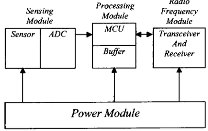
module,sensingmodule,and_processingmodule

[1],

as shownin Figure 1.

Sensing Module

Processing Module

Radio Frequency

MCU

Sensor ADC ? 4rt> Transceiver And Receiver Buffer

tk iL t i

[image:11.540.154.368.388.523.2]

Power Module

Figure 1.1 Architectureofawireless sensor.

The power module shown in Figure

1.1,

supplies the _energy to each ofthe other modules.

The sensingmodule_continuouslycollects

data,

convertsit from an_analogtoadigital _signal,

andthen passes itto the _processing module. The data is processed

by

the Micro Controller

The RF module isthe _only partthe _sensing device that is

directly

affected

by

other sensors

contending for access to a communication channel or a data collection gateway. It also consumes a significant amount ofthe overall_energyprovided

by

thepower module. In

fact,

studies inthepast have shownthat

transmitting

1 bitover 100 meters consumes_roughlythe same amount of_energy as _executing 3000 instructions

by

the MCU

[10],

which is

highly

significant. A plus side to the RF module is that its complexity, transmission rate, transmission range, reliability, etc., may all be adjusted to meet specific requirements and

therefore enhanced capabilities _may be sacrificed in order to conserve energy.

Many

RF

modules also have the _capability of _{operating in different energy} consumption _modes,

including

sleep,

idle,

receive, andtransmit modes [13].

The sleep mode, which will also be referred to as the OFF _mode, consumes a negligible

amount of_energyandis

typically

used

during

inactive periodsto conserve energy. The idle modeisthemode inwhich theRFcircuitisturnedONyetthe transceiverisnot_receiving or

transmitting

data. To switch from OFF to

ON,

an amount of spike _energy is consumed and has beenshowntobequite significant [18]. Asaresult,one must usethe_{energy conserving}

OFF mode _cautiously since _{switching between ON} and _{OFF may} result in a larger overall

consumption due to the spike energy. In the ON mode,

however,

the sensor can switch betweentransmitand receive modes without_{consuming any}spike energy.

Thetransmitmodeisused

by

the transceiver to send

data,

and consumes a significant amount

of_energyinadditiontothat consumedintheON mode.

Finally,

thereceive_mode, similarto the transmit mode, consumes _energy in addition to the ON mode _consumption,

however

3-consumes_onlya small amount of addition_{energy [19].} Alsonote thatthereceive mode and

the transmitmodebothrequire theuse ofthetransceiverand, therefore, cannotbe preformed

simultaneously.

Over the lifetime of a sensor, the majority ofthe sensor's _{energy is}

typically

consumed

by

the RF _{module, thus the} focus of a sensor or network operational model should aim at

understanding howthis module consumes _energy

during

the

OFF, ON,

andtransmit modes.

Also,

in a

"multi-hop"

network, where data is relayed through multiple sensors before

reaching the final

destination,

the receive mode should also be considered in the model.

Finally,

the spike _energy needs to be considered in a model so that _{switching between} the

OFF mode and the ON mode can be investigated under realistic _energy consumption

conditions.

1.2 Literature Review

on

Energy

Efficient WSN Operations

Many

methods for_reducinga sensor's_energyconsumption havebeen proposedin literature.

In general, these approaches can be divided into one of two categories. The first set of

approaches

indirectly

reducesthe amount of_energy spent

by

the RFmodule

by

_routing data

throughout a network _using the most energy-efficient paths.

They

focus on "multi-hop"

networks inwhich data_may

jump

from sensorto sensoruntil itreaches its final destination.

Inessence, thisset of worklooksat waystobalance dataflowsovertheentire networkinthe

steady state, such that the amount of _energy consumed

by

each sensor's RF module is

roughly the same. Optimal steady state solutions have been found for models _seeking to

for models _aiming at_maximizing the data retrieved overthe entire network

[6]

[12]. These

steady state models provide information abouthow data shouldbe disseminated throughout

the network on average overthe network lifetime andprovide innovative methods for how

WSNoptimization models _maybedeveloped.

Yet,

they

do not provide adequateinformation

that would enable sensors to make decisions in real time and do not account for the spike

energy sincethe model is developed forthe _steady state,

i.e.,

no _{switching between OFF}and

ONmodes.

The second set ofapproaches taken to reduce a sensor's _energy consumption is to

develop

efficient Medium Access Control

(MAC)

protocols that create more efficient transmission

schedules

by

_utilizing the different _energy modes of the RF module. These protocols

[13][18][19][20]

mostlymakedecisions withregardto _switchingthe RF module of a sensor

between transmit mode and OFF mode and _generally achieve significant performance

improvementswhencomparedtoschemesthat

keep

the sensorin ONmode ortransmitmode

at all times. This set of_work,

however,

does notaccountforthedatathat hasbeen collected

by

the _{sensing circuitry} and often overlooks the spike _energy consumed. In addition, these

protocols focus on

heuristically finding

the compromise _among the various _energy

consumption factors but lack a theoretical foundation to compare actual performance with

maximum performance capabilities.

2. Problem Description

Theapproaches reviewed intheprevious section offerinvaluablelessonsonhow energycan

be _conserved, either

directly

or

indirectly,

by

the RF module. Yet

they

are not capable of

determining

how each networked sensor should turn

ON,

OFF,

or transmit over _time, such

that the network_capability is maximized. For

instance,

the firstapproach,

least-energy

data

flows,

provides a good method for _modeling a sensor network environment,

i.e.,

the

optimization model.

Yet,

theoptimal results obtained arelimited since

they

lackinformation

aboutthebehaviorofthesensors overtime. As forthe second approach, theMACprotocols

are capable of_{conserving energy}

by

_making the sensors behave more _efficiently overtime.

However,

these protocols are based on single sensor power consumption models and

therefore do not _accurately incorporate the impact of _contending sensors in a network

environment. The

inadequacy

ofbothoftheabove approachesis that

they

attempttosolve a

specific problemratherthan

looking

atthebroadchallenge.

Theresearchinthis thesisattemptstomaximizethe_capabilityofaWSN

by

determining

how

the optimal _energy efficient

behavior1

ofindividual wireless sensors can be duplicated in a

contention dominated network environment.

Using

the contributions of other research as

reference, various _modeling approaches are used to determine the optimal sensor

behavior.

First,

an _analytically derived model is developed to determine the optimal single sensor

energy efficient behavior given an optimal _environment,

i.e.,

no contention _among sensors

whentransmitting. Two schemes:

first,

sensorsarekept ON at alltimesand_second, sensors

are switched between ON and OFF _modes, are examined in this model. For the second

1

scheme where sensors are turned ON and

OFF,

the effect of

buffering

data for a variable

period oftime and _allowing sensors to transmit at the most efficient time is explored. In

addition, the spike _energy and other realistic _energy parameters are accounted for in this

model.

This single sensorbehaviormodel, dueto the fact that itrepresent the ideal case, serves as

the theoreticalbounds incomparisontoresults obtainedina network environment andresults

obtained viasimulation models. Thisthesisproposes amixedinteger programmingmodelin

a dynamicregime. Thismodel, which accountsforrealistic _energy consumption parameters

and

buffer,

determines the optimal ON/OFF/transmission schedule, or

behavior,

of each

sensor over time. These results _may then be used to better understand how a contention

dominated network environment affects_{the optimal, contention-less,} single sensorbehavior.

After

developing

a baseline contention model _{solution, the} effect of independent factors

including

buffer size, arrival _pattern, service _capacity, network _{connectivity,} and _receiving

duty

cycle are evaluated with respectto thebaselinemodelcapability.

Knowing

the optimal transmissionschedules overtimeenables thisbehaviortobe converted

to a distributed _{decision making} heuristic. A heuristic ofthis type is a set of rules that

enables a sensorto

independently

schedule whento turn

ON,

turn

OFF,

andtransmit inreal

time. It isanimportant_extension,asitwill enable asensortobecapable of_adjusting toreal

world changes on-line. Future research _{may include} the development of a MAC protocol.

To conclude this _research,

however,

simulation results for sensors controlled

by

a

3. Optimal Sensor

Behavior

The analyticallyderived model usedto investigatethe optimal single sensor _energy efficient

behavior will be discussed in this section. This model is developed _assuming an optimal

communication scenario.

Therefore,

thediscussion begins withadescription ofthemodel's

optimal conimunicationscenario,variables, and_energyparameters. Thiswill be followed

by

a comparison of_{two schemes,} one inwhichthe RF module ofthe sensoris ON at all _times,

and a second schemeinwhichtheRFmoduleisturnedONandOFF. Thegoal ofthismodel

is to investigate the optimal sensor behavior over time when

buffering

of sensed data is

allowed.

The best communication scenario for a sensor in a sensor network is to always have full

access to a data collection _gateway whenever it is needed and to have _every bit ofdata

transmittedreachthedestination successfully. Full accesstoadatacollection_gatewaycould

be achieved through other _sensors;

however,

this _{multi-hop capability} is ignored in this

model. This best scenario is assumed forthis model and the amount ofdata a sensor can

sense and transmit to adatacollection _{gateway (or gateway in short)} given_{the total energy,}

elol , available for the sensor, will be investigated. Let thetotal amount ofdataretrieved

by

the_gateway beR=

\U(t)dt

, where

U(t)

<// istheamountofdatatransmitted

by

the sensor

at_timet, and jj. is themaximumtransmission_capacityofthesensor. Also let k< /j. bethe

fixed arrival rate of the sensed data. For the _{different energy} consumption _parameters,

keeping

the RFcircuitON foronetimeunitis

designated,

_e0, theenergy for

transmitting

one

andthe_energyconsumedfor_switchingtheRFcircuitfrom OFFtoONis

designated,

e.

, also

referredtoasthe spike energy.

3.1 Continuous

ON Scheme

First consider the case where a sensor has its RF circuit remain ON at all times. The

following

claim showsthat the totaldataretrieval underthis_scheme,

Rcomon

_,isindependent

oftheamount ofdatathatisretrievedateachtimeperiod.

Theorem 1: The maximum amount of data a sensor can retrieve when a sensor is kept

Continuously

ONoveritsentirelifetimecanberepresented as:

RCotON

=

(31)

Proof: Let Tbethelifetimeofasensor.Thenthe total_energyconsumed,_elol, andtheamount ofdata

toberetrieved,

Rc0>uON

,are

1 i

=_esT+e0T+

et

ju(k)dk

and

RConiON

=

ju(k)dk

lc=0 k=0

Basedontheassumptionthatno senseddataislostandthe_{buffer may}notbeover

filled,

one

candeterminethat

IT-B<

[u{k)dk

<_XT

A=0

where,B, isthebuffersize ofthesensor. Let \U(k)dk=XT-8

; where 0<8<B. Onecan

k=0

therefore rewrite, etot=

esT+e0T+et(kT-S), whichleadsto

T=

jt2L

+

eIS__

es+e0+ e,A

Now,

one can rewrite _RcomON as afunctionof8,

RContON

= kT - S

etotk + etkS es8 + e0S + etkS

es +eo + et^ _es + _eo + et?i

=

etot^ _{~S(es +eo)}

es+eo+etx

Clearly, RcontON

ismaximizedwhen,

8

0 andthemaximumdataretrieval

k

^ContON

~

7*eto/ es+e0+etk

I

This result is dueto the simple fact that the cumulativeamount ofdatathatcanbe collected

at _any point in time cannot be greater than what has been sensed.

Apparently,

one _way to

achieve this optimal performance is

by

_simply

letting

U(t)

=

k,

Vr_>0

,

i.e., transmitting

whatever is sensed

immediately

upon arrival. This policy is referredto as the "Continuous

ON"

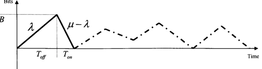
Bits ti

B

X

\>--'-N..,'X

Toff

1T [image:20.540.55.476.59.171.2]

on Time

Figure 3.1 Bufferutilizationforasensor_turningONand_{OFF periodically}throughits lifetime.

3.2 ON/OFF Scheme

In contrast to the Continuous ON scheme, one _may utilize the buffer space, to

temporarily

storethesenseddatawhiletheRFcircuitis

OFF,

andthen turn the RFcircuitONto_transmit,

perhaps at full _capacity forone or _many consecutive _{time periods,} as shown in Figure 3.1.

To understand what constitutes an optimal

behavior,

the _energy expenditure of a general

network without _any contentions,

i.e.,

sensor can transmit data whenever it

desires,

is

analyzed, given a fixedamount of

data,

R

,toberetrieved. The

following

equation represents

thelowerboundon_{the total energy,}

^lb

_,consumedunderthissetting:

R R

eLB=ep+es,-₊

eo +etR

k jU

To minimize the spike _energy, a single OFF/ON cycle is _assumed, which leads to a single

spike in_energy,

ep

,

i.e.,

the firstterm ofthe aboveequationabove. The secondterm ofthe

R

equation,es

y

, represents the minimum amount of sensing energy that could be used,

by

assuming that the sensor will _completely drain its buffer and _completely consume all ofits

energy at_preciselythe same time.

Assuming

themaximum transmit_capacity,M, is utilized

R

for_every

transmission,

the third

term,

eo , representsthe minimum ON energy consumed M

by

the sensor.

Finally,

theamount of_energyto transmit R units ofdata is _simplyafactorof

theamount ofdataandthe_energyconsumedper

bit,

etR.

Basedon the equationabove, one can derive the

following

resultforthe optimal amount of

datathatcanberetrieved,

RON/OFF

,

by

anON/OFFschemeina network without contentions.

Theorem 2: The largestamount ofdatathatcouldberetrieved

by

asensor_usingandON/OFF

scheme, RON I OFF-IS

RON I OFF ~

ietot-ep)

es eo

+ +.,

(3.2)

k /U

Proof: Considerthelower bound_energydescribedabove,

,

RONIOFF

RON

I OFF

R +_eo

etRON/ OFF

A Ll

'-tot ^ _*LB ~

ep

^"s

es eo etot

-ep

+

&ON

I OFF

~7~_{+ +}

et V A J*

RONIOFF

\etot

-ep)

k fi

A logical progression from this

finding

is to determine whether there exists a simple

answeris_yes,

by

having

thesensor complete one and_onlyone"full ON/OFF cycle."

Afull

ON/OFF cycle starts with a sensor

being

OFF,

_{storing any} data it senses in its

buffer,

and

then _{iluTiing ON} and

transmitting

_continuously until the buffer is empty. Note that the

optimal

RONIOFF

is achieved ifthe sensor's _energy is _completely expended at _exactly the

same time the buffer is expended. To complete a full ON/OFF _cycle, a buffer of sufficient

capacityisrequired.

Although the cost of _memory has become _relatively

inexpensive,

it is still _necessary to

investigatetheactual amount of storage requiredtocomplete afull ON/OFFcycle. In

fact,

a

buffer size of this magnitude _{may lead} to an unacceptable amount delay. A natural

progression of Theorem 2 allows the derivation of the buffer size required to

achieveRONIOFF.

Corollary

1: Let

B*

represent the smallest buffer size required

by

a sensor to achieve its

maximumdata retrieval _{capability in} a contention-less _environment,

ande^

>0

,

then,

*

(/J-Wetot-ep)

D =

e0+Me,+_jes

(3.3)

Proof: Considerasensorthathasabufferof size

B,

andfollowsafullON/OFFtransmissioncycle.

Thetotaldataretrievable,

R,

achievable

by

thissensoris

R=d

B ^

H-X)

Giventhat R^

ron/off

andTheorem

2,

itcanbeconcludedthat

etot

ep

1 1

=R

ONIOFF >R =ju

-es+/uet+e0

B

yH~kj

(etot-epr(M-A)^B*^B

es+fiet+e0

Basedon Theorem 1 and Theorem

2,

one can also determinethe condition (as afunction of

the_energyparameters, arrival _rate,and service_{capacity) for}whichtheON/OFF schemewill

retrieve agreater amountofdatathan theContinuous ON scheme, _orR*ON/OFF >

R*Co

^ContON

Corollary

2: A sensor_usingtheoptimalON/OFF schemewillretrieve a greater amount ofdatathan

theoptimalContinuous ONschemeifand_{only if}

, M

~ A, .

ep

^

etot

(

)

H e0+es+ etk

(3.4)

Proof: ConsidertheoptimalContinuous ONscheme

(3.1)

andtheoptimalON/OFF scheme(3.2).

k

\etot

ep)

_

D* _

V

~

KON I OFF - KContON

es eo

k //

J

\etot ~

eP

)

k

e0+es +etk tot

>

e0+es+etk 'tot

=> -e_ >

e0+es+etk

^eD ^etot(-

)

Ktot

ess eo + +e.

k jU

-tot

n ^tOtV ' .

3.3

Comparison

of

Continuous

ON

Scheme

and

ON/OFF Scheme

The above results canbeusedto determine whether _employing an optimal ON/OFF scheme

is beneficial (as compared to the Continuous ON scheme), and to detemiine the maximum

amount ofdatathat _{may be}retrieved

by

_usingthis ON/OFF scheme. Howevera _significant,

or perhaps unrealistic, buffer space _may be required to construct a single ON/OFF cycle

throughout the sensor lifetime.

Moreover,

asthe buffer size

increases,

the _queuing

delay

of

the sensed data also

increases,

which _may pose yet another problem from the application's

perspective. One waytoaccommodate a smallerbuffersizethan theone showninFigure 3.2

is to have multipleON/OFF cycles foran ON/OFF scheme. One can_easily derive the total

[image:24.541.53.503.454.650.2]

amount of retrieved data for a multiple ON/OFF cycle scheme based on

(3.2)

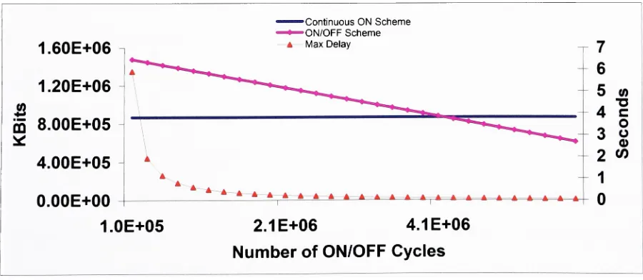
and (3.3).

Figure 3.2 exhibits the amount of data that can be retrieved

by

_using the two schemes:

Continuous ONandON/OFF withrespectto thenumberofON/OFF cycles. The maximum

queuing

delay

associatedwith_using such ON/OFF schemes isalso shown in Figure 3.2 and

isalso plotted withrespectto thenumberofON/OFFcycles.

1.60E+06

1.20E+06

fi

8.00E+05 __

4.00E+05

0.00E+00

ContinuousON Scheme ON/OFFScheme

Max_Delay

1.0E+05 2.1E+06 4.1E+06

NumberofON/OFF Cycles

Figure 3.2 Data retrieved

by

_using the Continuous ONscheme and the ON/OFF scheme with

different numbers ofON/OFF periods; also shown is the maximum

delay

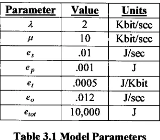
associated withthe ON/OFFscheme.

Parameter Value Units

X 2 Kbit/sec

V 10 Kbit/sec

es .01 J/sec

eP .001 J

e, .0005 J/Kbit

eo .012 J/sec

[image:25.540.193.352.59.198.2]

etot 10,000 J

Table 3.1 ModelParameters

To plot Figure

3.2,

the set of parameters shown in Table 3.1 were considered. These

parameters were derived based on the information provided in

[4]

[13],

for the purpose of

exhibiting the realistic performance achievable

by

a wireless micro-sensor. Sensors for

different sensing purposes, whichhave adifferent RF

implementation,

_{may have} a different

set of parameters.

However,

thegeneral performance trendis foundto remain consistentfor

a large _variety of parameter choices. Given the set of parameters shown in Table 1, the

maximum possible retrievable amount of data is found to be about 1500 Mbits for the

ON/OFF scheme with a single ON/OFF cycle (not shown in Figure

3.2),

and about 870

Mbits (the constant line shown in Figure

3.2)

for the Continuous ON scheme. The buffer

size and the _queuing

delay

associated with the single ON/OFF cycle scheme however are

unrealistically large

-about 1.2 Gbits and 7 hours worthofdelay.

By

stretchingthe sensor

operation into more and more ON/OFF cycles, it is foundthatthe retrievable data decreases

linearly,

while the maximum

delay

decreases much more _quickly as a reciprocal functionto

the number of ON/OFF cycles. Notice that the ON/OFF scheme is capable of_retrieving

moredatathantheContinuousONschemeuntilthenumberofON/OFFcycles reaches about

4.2 million. Atthis point abufferof_only 160 bitswould berequired, which resultsin about

scheme is at, perhaps, 1 million ON/OFF cycles, where a significant amount ofdata (1340

Mbitsout of possible 1500

Mbits)

canberetrieved whilethe

delay

isdroppedsignificantly to

about 500millisecondswiththebuffersize

being

about 1 Kbit. Thisset ofnumerical results

suggeststhe _superiorityof an ON/OFFscheme overtheContinuous ON scheme, evenwitha

quitelargenumber ofON/OFFcycles.

4.

Networked Sensor

Behavior

The analysis in the previous chapterhas suggest that a sensor should store as much sensed

data as possible and then transmit at full _capacity, as

long

as the sensor is capable of

transmitting

toadatacollection_gatewaywheneverit desires. Inanetworksetting,

however,

multiple sensors_maycontendforthe same wireless communication channel ofeachgateway;

thus, the full ON/OFF cycle described in the previous section_may not be feasible. In this

chapter, the optimal, contention

dominated,

networked sensor behavior is investigated

by

consideringa mixedinteger programmingmodel. Thistaskisaccomplished

by

_analyzingthe

behavior ofthe sensors in a baseline model. With the behavior ofthe baseline contention

model solution

determined,

theeffect ofthebuffersize, arrivalpattern,network_{connectivity,}

and service _capacity, are evaluated with respect to the baseline model behavior and

capability.

The _{interaction among gateway sharing} sensors is modeled _using a bipartite _network, as

shown in Figure

4.1,

in which one set ofnodes represents the sensors and are connected to

the other set of nodes _representingthe gateways. This simple bipartite structure allows the

focusto beplaced onthe ON/OFF behaviorofthe sensorsthatare _{contending for}a common

gatewayaswell as those that_{may be} serviced

by

multiple gateways. Althoughitseems like

a simplified sensornetwork, thebipartitenetwork modelcanbe viewed asthe

building

block

JUy

=_Maximum

transmission_capacityfrom

sensor_jtogatewayipertimeperiod.

etj

=

Energyrequiredtotransmitone unit

ofdata fromsensor_jto_gatewayi.

Sensors _Gateway

Decision Variables:

, 1,ifsensorjis ONduringtime Status_ji < periodt

A'

{

{

0,otherwise

1,if gatewayiservices sensor_{j during}

timeperiodt

0,otherwise

1,ifsensor_jswitchesfrom OFFtoON duringtimeperiodt

0,otherwise

U,.,=_Amount

ofdatatransmittedfromsensor_j

ii

to_{gateway iduring}timeperiodt.

elolj=Initial_energyofsensor_j

epj=Spike_energyof sensor_j

ej=Idleenergyof sensorj

[image:28.540.43.450.46.283.2]

Bj

=Buffersizeof sensor_j

kj

=Senseddataarrivalforsensor_j

Figure 4.1 The sensor-gateway bipartitenetwork model.

Tounderstandin depth how contending sensors shouldbehaveover_time,

"time"

isadiscrete

variable in the mixed integer programming model. The notation defined in the previous

section is

followed,

and extended with subscripts to indicate the associated

sensor

{j; j

=

\,...J}

, gateway

{/';

i =

1,.../}

, andtimeperiod

{t;

t =

\,...T}

. Figure 4. 1 showsthe

variablesand constants that defineall datathat willberepresented inthemodel. Figure 4.2

defines the objective and constraints of a

fully

comprehensive mixed integer program.

Notice that the arrival rate is now generalized to

kp

, enabling a variable amount ofdata to

arrive atdifferenttimeperiods. Inadditionto_creatingavariable

Ul]t

thatcorrespondsto the

amount of data transmitted from sensor

j

to _{gateway i} at time _t, three

binary

decision

variables are introduced. The first decision variable,StatusJt , is used to represent whether

sensory is ON

(1)

or OFF

(0),

attime t. In order for a sensorto transmit

data,

the sensor

/

mustbe

ON, Status,-,

=

1,

attime tanditmusthaveaccesstoa_gatewaywhich means one of

19-its data_paths,X_iJt, must equal 1 andthe rest mustbe

Xikt

=

0,

V&* _/ . To accountfor the

spike_{energy, the} value of

ZJt

is set

Zjt

= 1 _whenthe

sensoryturns ON attimet after

being

OFF at time _t-\, and remains 0 otherwise. It should be noted that the combination ofthe

binary

variables with the linearvariables

UiJt

ina single _model, results inthe mixedinteger

propertiesoftheproblem.

The mixed integer programmingmodel ispresented inFigure 4.2. Notice that the objective

function of the model is to maximize the total data retrieved

by

the network given a

maximumtime T. This will result in creatinga

binary

search process overtime

T,

between

feasible andnon-feasible modelswith

differing

valuesofT.

i"=l j=\ r=l

suchthat,

j=i

Vi&Vf,

Status,

Z^Xy,, y/&vr,

Z_, >Status

Jt

-Status

7(,_1}, V/&Vf,

U1Jt<rlIJXIJt

V/&V;&V?,

1=1 =1 1=1 (=1

\fj&VS=_1,2,-T

,

i=i 1=1 i=i

V/& VS=_1,2,..J ,

TIT T

Thisobjectivemaximizesthe totaldatatransmitted.

Sensorsarelimitedtoaccess _{1 gateway}at atime.

SensorsmustbeONtoaccess agateway.

This decidesthespikeenergystatus of all sensors attime t.

Sensorscannottransmitmorethanthecapacityofthelink.

Sensorscannottransmitmorethanwhathas beensensed.

Sensorscannot overfillthebuffer.

Sensorscannot use moreenergythan theinitialtotalenergy

epJ^ZJt +XXe'-y(/' +eoj^StatusJ'-e>o',j' V/' /=1 <=1 t=\ t=\

[image:29.540.45.494.350.597.2]

Statute{0,1},V/&Vr; J^e&lKVz&vy&V/; ^,>0,vi&vjr&V/.

4.1

Solution

of

Small Networks

At first _{sight, the} problem presented in the previous section has a lot of similarities to a

Bipartite

Matching

Problem which has been dealt with in

literature

by

_usingdifferent types

ofpolynomial-time algorithms [9]. In _reality,

however,

theproblem is much more complex,

as sensors are _contending for resources and buffer overflows are not allowed. This

contention andfinite storage resource creates aNP-Hard MIPproblem,

i.e.,

optimalitycan be

achieved in an exponential number of steps based on the

input,

which encompasses the

generalized knapsackproblem [7].

Finding

the _globally optimal solutionfortheMIP model

as a comprehensive solution approachis_{computationally}prohibitive.

Due to the

difficulty

and time required to solve the MIP model, a _very small _network, 4

sensors and 2 _gateways, was chosen for the base scenario topology. The sensors in this

scenario were set _up such that

they

were

fully

connected, meaning all sensors shared access

toboth_gateways,andthesame _energyparameters asshownin Table 3.1 were consideredfor

all sensorswiththe

following

assumptions:

1. _{The sensing energy} consumption is assumed to be zero since it is consumes a

negligible amount of_{energyconstantly}overtime.

2. The buffer is fixed at 24

Kbits,

which was determined from the single sensor

behaviormodeltobea

"reasonable"

buffersize.

3. _{The energy}is scaleddownto0.2joulestocontrolthesize ofthemodel.

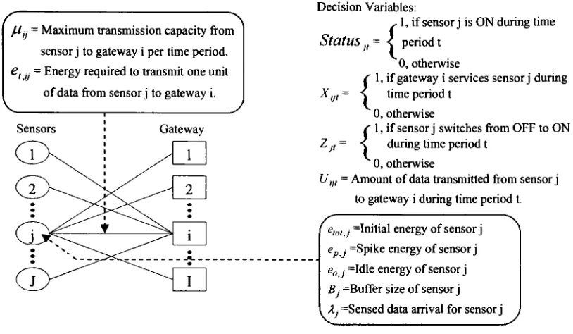
The spikedcurve in Figure4.3 shows the transmission scheduleof a single senorfrom a4-2

network. The sensor, whose transmission schedule is _shown, was capable of_retrievingthe

21-maximum amount of data over its maximum lifetime. Figure 4.3 shows the transmission

schedule over the maximum possible lifetime of a sensor on one _exemplary simple network

thathas 4sensors and2 gateways. The linesplottedinFigure 4.3 representthetransmission

rate used

by

one ofthe sensors (regardless ofwhich _gatewaythe data is sent _to), whenthe

ON\OFFscheme andthe Continuous ONscheme are used. Noticethat

by

_usingtheON/OFF

scheme, the sensor has a much longer

lifetime,

61 time periods as compared to the 15

achieved

by

the sensor _using the Continuous ON scheme. Further comparing the total

amountofdataretrieved via_{this sensor,}whichisthesum ofthetransmitteddata over_{time, it}

is found to be 110 Kbits for the ON/OFF scheme

-a 267% improvement over the

Continuous ON scheme that is capable of _{collecting 30 Kbits.} A

key

reason that the

ON/OFFscheme is ableto retrieve much moredata giventhe same_energy constraintsis the

use ofbuffer _space, which allows transmission at full capacity almost _every time the RF

circuitisturned ON.

-^ON/OFF Behavior

-Continuous-ON Behavior

mumm^r*mm

1 5 9 13 17 21 25 29 33 37 41 45 49 53 57 61 65 69

[image:31.541.62.475.436.662.2]

Time

(sec)

Figure 43Datatransmittedovertimeforone ofthesensors ona4-2 (Sensorsto

Gateways)

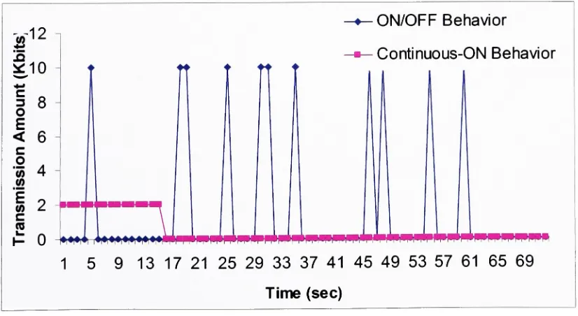
Figure 4.4 displays the buffer usage over _{time, corresponding} to the optimal ON/OFF

transmission schedule that was plotted in Figure 4.3. Notice on two occasions (at time 15

and time

29),

the sensor's buffer comes _nearly full and _{is followed}

by

two consecutive

transmissions,

which _{significantly} reduces the buffer's content. This behavior does not

exactly duplicate the ON/OFF behavior found _{analytically,}

however,

it does provide

evidencethat thesensoris_seekingtobehaveintheoptimal

fashion,

i.e.,

fullON/OFFcycles.

Full ON/OFF cycles_maynotbe_completed,

however,

duetocontentioninthenetwork. Also

notice that the buffer is not _completelyemptiedbefore the sensorturns OFF. This behavior

may be attributed to the sensor

being

incapable of_{completely empting its} buffer

during

a

single ONperiod unless ittransmitsbelow itsmaximumtransmit_capacity foratleast one of

its transmissions. As a result, rather than

transmitting

at less than full _capacity, which is

inefficient,

thesensorbuffersthedata.

Buffer Usage Over Time

30

!

3

25

j2 20

c

B

15

c

O10

__ 5 it

3 n

OQ U i ii I I I I I I I [ I I I I I I I II I I I I I I M II I I I I I M I I I I ! I I I I M M I I II I I l I I I I I I III I I II I I I

1 5 9 13 17 21 25 29 33 37 41 45 49 53 57 61 65 69

Time

(Seconds)

Figure 4.4 Bufferutilization overtimeforone ofthebasemodel sensorsinabipartitenetwork

demonstrating

ON/OFF behavior. [image:32.541.46.480.406.640.2]

23-4.2

Effect

of

Arrival Pattern

Wireless sensor networks _may be used in _many different _{applications,} each ofwhich _may

havea_considerablydifferentarrival patterns overtime. Fora given_application,onepossible

arrival pattern_may consist of periodsinwhich alarge amount ofdata is sensed followed

by

long

inactive periods. The results above show that an ON/OFF scheme can achieve

significant data retrieval improvements over the Continuous ON scheme, assuming all data

arrives constantly. To determine how the arrival patterns would affect the amount oftotal

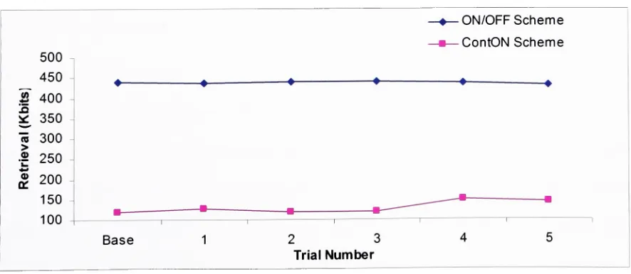
dataretrieved, thedifferentarrival patterns showin Table 4.1 are consideredforthe same4-2

network. The resulting optimal data retrieval amounts

by

the ON/OFF scheme and the

Continuous ONscheme areplottedin Figure 4.5.

Trial Arrival Pattern(Kbits)

Base 2-2-2-2-2-2-2-2-2-2-2-2-...

1 4-0-4-0-4-0-4-0-4-0-4-0-...

2 6-0-0-6-0-0-6-0-0-6-0-0-...

3 10-0-0-0-0-10-0-0-0-_10-...

4 14-0-0-0-0-0-0-14-0-0-0-...

[image:33.541.169.367.342.439.2]

5 1g-O-O-O-O-O-O-O-O-_18-0-...

Table 4.1 Arrival Patternswith same average arrival rate(2 Kbits/Sec).

500

450 1"

400

* 350

NJ K) OJ

O

OI

O

150

inn

Base

-?ON/OFF Scheme

-n ContON Scheme

2 3

Trial Number

Figure4.5 The amountofdata retrieved

by

a4-2 bipartite network withrespectto thevarious [image:33.541.47.490.475.668.2]

As shown in the figure _{above, the} amount of data that can be retrieved is _relatively

insensitivetothedifferenttrafficpatterns considered. FortheON/OFFscheme, this is dueto

the buffer

being

capable of_absorbingthe arrivals.

Therefore,

as

long

as the amount ofdata

that arrived in a single period does not exceed the buffer size, the transmission schedule

won't change _much, and

hence,

similar amounts of total data are retrieved. For the

Continuous ON scheme, where data is transmitted

immediately

upon _{arrival2, the total}

amount ofdataretrieved isequal to the total amount ofdata arrivedthroughout the network

lifetime,

with one exception when the data sensed in the last time period is larger than the

maximumtransmission capacity. Thedifference in total data retrieval dueto the exception

will bemarginal as

long

as the sensorlifetime is muchlargerthan the inactiveperiod ofthe

traffic pattern. This is indeed the case inthe scenario considered in Figure 4.5. This set of

results exhibits _{that, for}at leastthe base scenarioconsidered, the ON/OFF scheme provides

robust performance with respect to fluctuations inthe data arrival pattern, and _consistently

outperformsthe Continuous ON scheme. An

interesting

extension relatedto this _studyisto

consider stochastic arrival rates.

4.3

Effect

of

Buffer

Size

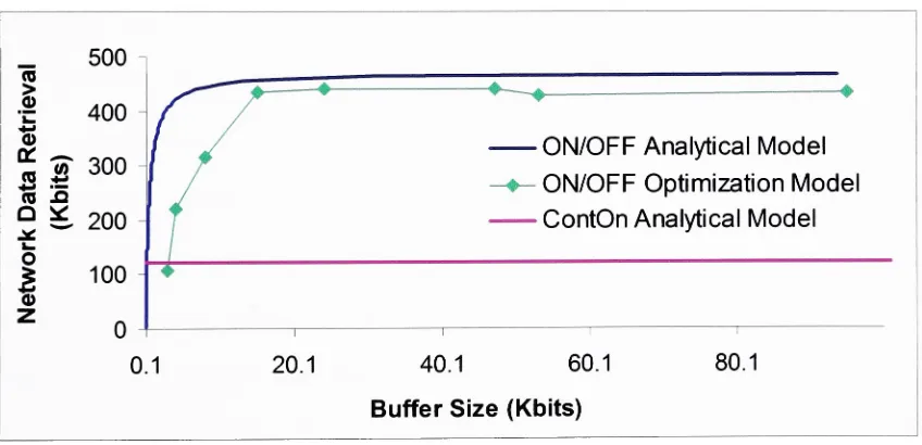
Figure 4.3 and Figure 4.5 demonstrate the significant performance improvements of the

ON/OFF behavior as compared to the Continuous ON behavior. These resultshowever are

basedon anetwork inwhich each sensorhas afixed buffersize of24

Kbits;

thus theimpact

ofthe buffer size in these figures is unknown. Figure 4.6 contains a plot ofthe total data

retrieved

by

the4-2 bipartitenetwork whenone uses an

increasing

buffersize.

Interestingly,

2

Incases where moredataarrives

during

atimeperiodthancantransmitted,theexcessdata isassumedtobe bufferedandtransmitted

during

thesubsequenttimeperiod(s).

the total dataretrieval increases _{significantly}as the buffer size

increases

whenthe buffer is

small (less than 18

Kbits),

and saturates to about 430-440 Kbits after that. Notice that in

Figure 4.4 the actual buffer space _utilized, i.e. the buffer size minus the residual buffered

data,

iscalculatedto be _{approximately} 17-₂₀

Kbits,

which is consistentwiththe buffersize

requiredtoretrievethemaximum amount ofdata fromtheoptimalbehaviorsection. Several

other small networks were examined and the same performance trend with respect to the

buffer size was observed. This leadsto a logical question ofwhetherthe total dataretrieval

of440 Kbits is indeedthemost one can collect no matterhow largethebuffer size is. This

question was answered _using the analytical results fromthe optimal behavior section which

determinedthisamount of retrievalto_{be very}closetooptimal.

500

re > 01

400

<-> 01 Ul

tfl 300

(U 4-> re _3

Q

_ *

200

o

|

0> 100

ON/OFFAnalytical Model

ON/OFF Optimization Model

ContOn Analytical Model

0.1 20.1 40.1 60.1

Buffer Size

(Kbits)

[image:35.541.45.469.350.555.2]

80.1

Figure 4.6 Dataretrieved

by

a4-2 bipartitenetwork with respecttobuffersize solved_optimally

for ON/OFFscheme,and_{analytically for both ON/OFF}schemeandContinuous ONscheme.

From Figure 4.3 it was deteiminedthat the networked sensors are not capable of_achieving

full ON/OFF cycles due to contentions with other sensors.

If, however,

all ofthe sensors

better than the networked sensor scenario in terms ofthe _energy usage and the total data

retrieval. A characteristic curve is drawn based on the optimal

behavior,

in Figure

4.6,

to

exhibit the performance that could have been achieved

by

the four sensors ifthere were no

contention. Thecharacteristic curve is derived basedon equation

(3.2)

and equation

(3.3)

as

done for Figure

3.2,

yet here it is scaled _up to correspond to four sensors. Alsoplotted in

Figure4.6isthe total dataretrieval achievable

by

theContinuousON scheme as areference.

Many

interesting

observations canbe made from Figure 4.6.

Foremost,

one shall note _that,

as

long

asthebuffersize isnot_{too small,}the total dataretrieval

by

thefoursensors in_reality

(with contention) is _verycloseto what

they

couldhave retrievediftherewere nocontention,

i.e.,

the best

they

cando. In

fact,

by

_examiningthe transmissionschedule of_{the sensors, the}

contention _amongthe sensors is found to be severe (sensors

frequently

switch between ON

and OFF states and

hardly

utilize the full transmission _capacity) when the buffer size is

small, and _gradually lessens as the buffer size increases.

Increasing

the buffersize reduces

the contention because it allows the sensors to _{stay OFF}

longer,

_allowing other sensors to

access _{the gateway,} and in a _sense, alternates the transmissions. The same performance

trends, as_above, are again observed when_consideringother simplebipartite networks. This

suggests that one needs _only a moderate buffer to retrieve an amount ofdata close to the

largest possible retrieval amount even for _contending networked sensors. The analytical

results seem to serve as a tightbound and agood approximationto whatnetworked sensors

can achieve_usinganON/OFFscheme.

4.4

Effect

of

Network

Service

Capacity

The total network retrieval _capability with respect to the maximum network service

capabilityper second is displayed inFigure 4.7 fora scenario whichhad five

fully

connected

sensors and three gateways. Maximum network service _capability per second is defined as

the maximum amount ofdatathatcanbetransmittedout ofthenetwork per_{time period,}

i.e.,

the total number of gatewaystimes the maximumtransmission_capability ofthe sensors. In

each of the _trials, the maximum network service _capacity was adjusted

by increasing

the

maximum transmission _capacity of each sensor

by

one Kbit. All of the same _energy

consumption parametersastheprevious4-2 models are again considered except forthe total

energyof_{the sensors,} which was increased to 0.5 Joules.

Also,

to ensure that the effect of

sensor contention is demonstrated (at least for the low maximum network service _capacity

levels)

the buffer was reducedto 12

Kbits,

andthe arrival rate was increased to 5 Kbitsper

second.

_ 260

re

I

240

1

220

o 5 180

|

-160

E

140

g

120

100

ON/OFFScheme Network Retrieval

12 17 22 27 32 37 42

Maximum Network Service

Capacity (Kbits/sec)

[image:37.540.39.474.406.619.2]

47

Figure 4.7 Networkretrieval_capabilityof a5-3 bipartitenetwork asafunctionofthenetwork's

In Figure

4.7,

when the service _capacity is low (15-18

Kbits)

the sensor is capable of

retrieving 128 Kbits - 139 Kbits

whichis_very lowcomparedto the expected_retrieval, -250

Kbits,

which was calculated

by

the optimal behaviormodel. This lowretrieval is dueto the

large arrival rate and the low service _{capacity requiring} the sensor to alternate _every other

transmission in order to

keep

its buffer from over flowing. When the sensor's status over

timewas

investigated,

itwas determinedthat aContinuous ONscheme was _actually utilized

due to the

frequency

ofthe sensor's

transmissions,

i.e.,

_every other second. Once the total

service _capacityreaches 20

Kbits,

the ON/OFFbehavior is utilized

by

the sensor and results

in a linear increase in total network retrieval before

leveling

off once the total service

capacity reaches the mid thirties.

Increasing

the total network service _capacity no longer

increases the total amount of data retrieved because the total network retrieval is now

constrained

by

thebuffersize.

Running

thesame scenario yet with larger buffersizes results

in the same curve except that it does not level off until the total network service _capacity

reaches ahigheramount.

4.5 Effect

of

Network

Connectivity

Network connectivity refers to the number of gateways that each sensor is capable of

transmitting

to. In networks _covering a small _area, it is feasible that each sensor would be

capable of

transmitting

to _every data collection _{gateway; this type} of_connectivity will be

referred to as

"fully

connected."

Along

with a

fully

connected network, Figure 4.8 shows

twoadditional networks withinwhichsensors_maynotbeabletoreach all gateways.

[image:39.541.89.436.50.184.2] [image:39.541.41.468.459.664.2]

Figure 4.8 Fromthe

left,

a

fully

connected_network,a

(2,2,1)

_network,and a

(3,1,1)

network.

Figure 4.9 shows the total data retrieval

by

the afore-mentioned three networks as the

individual sensor sizes increase. The separations betweenthe plots inFigure 4.5 illustrates

the impactofthe_{different connectivity levels} as well astheeffectivenessofeven a_relatively

small

buffer, i.e.,

18

(Kbits),

in_eliminatingthisdifference.

Moreover,

this plotdemonstrates

that a networkthat isnot

fully

connectediscapable of_retrieving thesame amountofdata as

anetworkthat is

fully

connected. Thisisa significant

finding

as itsuggeststhat a network's

connectivitycanbe_reduced,so astoreducethe

difficulty

of_{coordinatingthe sensors,} yetthe

network_maystillbecapable of_achievingitsmaximumcapability.

140

120

ra > _

%

100

a. _

* _J 80

o 3

|

* 60

Q)

Z ₄₀

ra

p 20

Full Connected

(2,2,1)

(2,1,2)

(1,3,1)

3 4 5 6 8 9 10 11 12 13 14 15 16 17 18

Buffer Size

(Kbits)

Figure 4.9 Total network retrieval with respect to buffer size for networks with

differing

5.

Heuristic

Development

InChapter

4,

the optimalbehaviorof a sensor ina network environment wasdetermined and

many

key

characteristics ofthisbehaviorwerediscussed. Theterm"behavior"referstohow

a sensor schedules itsRFcircuits to turn

ON,

turn

OFF,

andtransmitovertime inanetwork

environment.

Ideally,

each sensor in a physical network could be preprogrammed with its

optimal

behavior;

yet this cannot be done due to the

difficulty

of_solving the mixed integer

problemforeven small networks . More

importantly,

thispredeterminedbehaviorrequiresa

prior knowledge on the data arrivals _{and, therefore, is infeasible in} practice where

hard-to-predict sensed events happen in real time.

Consequently,

a _preliminary heuristic has been

developedtomimictheoptimal sensorbehavior. Theproposed heuristicconsistsoftwo sets

of criteria that will be used

by

the sensors and the

gateways4

to make decisions on the

transmission and the _receiving

behavior,

respectively, in an on-line fashion. The idea is to

have the sensors

independently

decide when to turn the RF circuit ON and request for

transmission, while each ofthe gateways will decide which _requesting sensor it will grant

access to. The goal ofthis distributive process is to have the network achieve close to the

optimal overall _capability as exhibited in Chapter 4. The flow charts ofthe two decision

criteria are showninFigure 5.1.

Several decision criteria determine the sensor behavior (the flow chart onthe left ofFigure

5.1)

andhowwelltheheuristicperforms.

First,

asensor willdecidewhento"TurnON?"

3

Anoptimal solution fora4-2 network withthe parameterT=50 was notfound

by

theCPLEXmixedinteger

optimizerafter10.23 hours.

4

The heuristic developed in this thesis assumes a 2-level hierarchical network, where the sensors will be

sensingand_{transmitting data}whilethegateways willbe_{only receiving data. A}straightforwardgeneralization

oftheheuristicisto implementthe twoset ofdecisioncriteria on each sensor sothata sensor will behave as bothatransmitterand a receiver asit_maybe inpractice.

Start

Receive requests or

data

<-V

Determine SensortoGrant

V

Sendgrant

Figure5.1 Sensor heuristic flowchart

(left)

and_{gateway heuristic flow}chart(right).

(the first decision

box)

based onthe bufferutilization,

i.e.,

howfull thebuffer is. Sincethe

sensoris OFFwhenitreachesthis

block,

theheuristic is designedtoremain intheOFF state

so as to conserve as much _energy as possible.

Only

when the buffer's utilization has

surpassedthe UpperBuffer Limit

(UBL), i.e.,

thebufferwill soonbe

full,

willthe sensorturn

ON andbegin_requestingaccessto a gateway.

Similarly,

the decision

block,

"Stay

ON?,"is

designed to

keep

the sensor inthe ON state as

long

as possible so as to distribute the spike

energy, consumed when

turning

from OFFto

ON,

overthemaximumnumber oftransmitted [image:41.540.67.438.49.417.2]

buffer

is_nearlyempty, indicated

by

examiningwhetherthebufferutilizationhas fallenbelow

the Lower Buffer Limit

(LBL),

thesensorwill _{stop requesting} accesstogateways and switch

to the OFF mode. The values ofthe UBL and LBL are determined based on the average

arrival rate ofthe sensor andthemaximumtransmission_capacityof_{the sensor,}respectively.

Ifthe decision is "yes"

for either the

"Stay

ON?" or "Turn ON?"

blocks,

the sensor will

determinethe highest _{priority neighboring gateway,} and senditatransmissionrequest. The

highest _{priority gateway} is the _gateway that is expectedto cause the sensor _consuming the

least amount of _energy ifthe sensed data were transmitted to it.

Determining

the highest

priority gateway and _sending it a request are the tasks performed

by

the sensor in the

"Request Gateway"_{block. The highest priority gateway}of_sensory is the_gateway i thathas

thelowestvalue of

cStaty

basedonthe

following

equation.

cStaty

=

Uy

*

euij

+

(Bj

-Uy)*

eu_j

V/ &

Vy

(5.1)

The variable

cStaty

estimates the amount of_energythat will be consumed

by

_sensory, if it

completely empties its

buffer,

Bj

(Kbits),

in a single ON time period and makes its

transmission of the

first,

Uy

Kbits to _gateway

/,

with the rest _equally transmitted to all

neighboringgateways. Theparameter

euj

isthe_energyconsumed

by

transmitting

oneKbit

ofdata from _sensory to _gateway /', and

e,_j

representsthe average _energy consumption per

Kbittransmitted

by

_sensory over all_neighboring gateways. This processof

determining

the

highest priority gateway and _sending it a request is performed _repetitively until _sensory is

granted access or until no more gateways are available. Notice that if the sensor is not

granted after_requesting accesstoall ofits_{neighboring gateways,} thesensorwillbackofffor

a short period oftimeandbegin_requestingagain_startingwithits highest_prioritygateway.

The decision of whether the sensor is granted access to a _gateway takes place in the

"Accepted?"

decision block. This decision is _actually made

by

the gateway. In

fact,

the

sensor will wait forthe _gateway to send back a "grant" _{acknowledgement,} and ifreceived,

the senor will transmit datauntil the utilization ofthe buffer falls below the

LBL,

atwhich

time the sensorwill turn off. The actual decision of_accepting the sensor performed

by

the

gatewayisexplained subsequently.

Ontheright side ofFigure 5.1 above, the flowchartforthe_{heuristic residing}atthe _gateway

is illustrated. The purpose ofthis part of heuristic is to allow _only a single sensor_y to

transmit to a particular _{gateway /} at _anypoint intime. In addition, the total channel access

allottedto _sensory over_time,

by

all ofits_neighboring gatewayscombined,must be sufficient

to ensure that_only aminimal amountofdata is lost. Sincethesensorsdetermine when

they

should begin to transmit without

knowing

other sensor's status, each _gateway needs to

choose the sensor that is expected to lead to more efficient _energy consumption. This

decision ismade

by

_comparingthe values of

tStattJ

based onthe

following

equationforeach

sensory thathaverequested accessto_{gateway /.}

tStaL = J

V/'V-/'

<5-2>

The sensor

j

with the largest

tStattJ

will be granted for access to _gateway

/,

since it is the

have the longest ON periodto disperse the spike energy. The parameter,

C,

(Kbits),

is the

current bufferutilization,

q~j

(Kbits/sec)

is theaverage service_capacityofsensory, to all its

neighboringsensors,and

kj

(Kbits/sec)

istheaverage arrival rateforsensory.

The heuristic describedabove _essentially pairs _up sensors and gateways, so that each sensor

once turned

ON,

will _{stay ON}forthelongesttimepossible. Noticethatintherealworldthis

process of_{pairing up may}take afew _signaling exchanges _among the sensorsand gateways,

and therefore consumes time and energy. The proposed

heuristic, however,

assumes such

process consumes much less time and _energy than those used for

transmitting

the sensed

data,

and therefore ignores both factors when _conducting the simulations.

Consequently,

whenever there is at least one sensor _{request, the} simulator will determine the "maximal

match"

betweenthe_requestingsensorsandthegateways.

5.1 Heuristic

Capability

Assessment

through

Simulation

To investigatethe effectiveness ofthe heuristicabove, thebehaviorof a sensor ina network

controlled

by

the heuristic and a sensor whose behavior was found _optimally

by

the MIP

model,werecompared. To makethis comparison,a4-2 networkwassimulatedandrun with

all ofthe sensors

having

identical power consumptionparameters, buffer sizes, dataarrival

rates and servicecapacitiesto those sensors usedto generatetheresults shownin Figure4.4.

Theresultsofthiscomparison arediscussed below.

Figure 5.2 demonstrates the bufferutilization overtime for a sensor ina 4-2 networkbased

onthe MIPmodel andfora sensor ina4-2 simulatednetwork controlled

by

theheuristic. In

35-Figure

5.2,

notice the similar behavior exhibited

by

one of the sensors under the two

experimental setups. In

fact,

the sensor,underboth _{setups, transmits}atotal of11 _times, and

transmitsatfull_capacityfor_every

transmission,

and as aresult,retrieves atotalof1 10 Kbits

ofdata.

25

MIP-Buffer Usage Over Time

-?

Heuristic-Buffer Usage Over Time

10 20 30 40

Time

(sec)

[image:45.541.60.469.185.377.2]

50 60 70

Figure 5.2 Bufferutilizationovertimeofasingle sensorina4-2 bipartite networkbasedonthe

MIPmodel andthesimulated networkunderheuristiccontrol.

The other network sensors under the two setups also exhibit similar _results, but may not

achieve _exactly the same data retrieval, which is _obviously expected. The overall

performance oftherespective networksisalso similar, whereatotalof440 Kbitsisretrieved

under the MIP model, and it is 420 Kbits forthe simulated network based on the heuristic.

The full ON/OFF behavior seems tobe moreprominent intheplotforthe simulated sensor.

One shouldhowevernotethat thebufferutilizationforthesimulatedsensorneverexceeds20

Kbits,

while it can reach 24 Kbits

-the full buffer size, under the MIP model. This

discrepancy

between the two setups leads to the _{slightly higher}performance achieved _using

The above results show an example ofhowa sensor

behavior,

similarto thatofthe optimal

behavior can be reproduced

dynamically

by

a sensor controlled

by

a heuristic. It is also

interesting

to investigate whether the performance trends of the wireless sensor network

previously exhibited in Chapter 4 can be also observed for the simulated network. In

particular, this thesiswillfocuson

investigating

theperformanceimpact dueto thesize ofthe

bufferat each sensor. For comparison, this set of results will beplotted in Figure

5.3,

_along

with the data points _already shown in Figure 4.6. As exp