This is a repository copy of Fep1d: A Script for the Analysis of Reaction Coordinates. White Rose Research Online URL for this paper:
http://eprints.whiterose.ac.uk/92529/ Version: Accepted Version
Article:
Banushkina, PV and Krivov, SV (2015) Fep1d: A Script for the Analysis of Reaction Coordinates. Journal of Computational Chemistry, 36 (12). pp. 878-882. ISSN 0192-8651 https://doi.org/10.1002/jcc.23868
[email protected] https://eprints.whiterose.ac.uk/ Reuse
Unless indicated otherwise, fulltext items are protected by copyright with all rights reserved. The copyright exception in section 29 of the Copyright, Designs and Patents Act 1988 allows the making of a single copy solely for the purpose of non-commercial research or private study within the limits of fair dealing. The publisher or other rights-holder may allow further reproduction and re-use of this version - refer to the White Rose Research Online record for this item. Where records identify the publisher as the copyright holder, users can verify any specific terms of use on the publisher’s website.
Takedown
If you consider content in White Rose Research Online to be in breach of UK law, please notify us by
Fep1d: a script for the analysis of reaction
coordinates
Polina V. Banushkina and Sergei V. Krivov
∗Astbury Center for Structural Molecular Biology, Faculty of Biological Sciences, University
of Leeds, Leeds LS2 9JT, United Kingdom
E-mail: [email protected]
Abstract
The dynamics of complex systems with many degrees of freedom can be analyzed by
projecting it onto one or few coordinates (collective variables). The dynamics is often
described then as diffusion on a free energy landscape associated with the coordinates.
Fep1d is a script for the analysis of such one-dimensional coordinates. The script allows
one to construct conventional and cut-based free energy profiles, to assess the optimality
of a reaction coordinate, to inspect whether the dynamics projected on the coordinate
is diffusive, to transform (re-scale) the reaction coordinate to more convenient ones, and
to compute such quantities as the mean first passage time, the transition path times,
the coordinate dependent diffusion coefficient, etc. Here we describe the implemented
functionality together with the underlying theoretical framework.
Keywords: reaction coordinate, free energy profile, diffusion, cut free energy profile, dimesionality reduction.
Introduction
With the growing number of experiments and the steady progress in the simulations of different biological, physical, chemical processes the rigorous quantitative analysis of the obtained data becomes all the more important. The complex nature of the processes and the large size of data sets generated by simulation and experiment make the development of automated analysis tools very important, practically and conceptually.
One popular method of such a data analysis is the projection of multidimensional coor-dinate space to a one dimensional reaction coorcoor-dinate (RC). During such a dimensionality reduction some information is inevitably lost. The optimal RC should absorb all the im-portant dynamical information contained in the other degrees of freedom, so they can be neglected. Then the free energy profile (FEP) constructed along the optimal coordinate together with the determined diffusion coefficient can give an accurate description of the system dynamics as diffusion on this free energy surface. Examples of such dimensionality reduction can be found in different fields: order parameters in physics,1,2 physicaly based
re-action coordinate in single molecular experiments3,4 and molecular dynamics simulations,5–11
biomarkers in medicine,12 chess game.13
In protein folding simulations the following RCs are frequently chosen: the root mean square distance from the native structure, the number of native contacts, the radius of gyration. In many cases, however, such coordinates can hide the complexity of the dynam-ics,2,14 in particular the barriers between states and make the dynamics subdiffusive.15 A
number of methods to construct good, more sophisticated reaction coordinate have been sug-gested8,16–22 and the analysis of the determined RC becomes as important as the description
of the dynamics.
rather than sub or super diffusive; transformation of the putative reaction coordinate to another, more convenient one, for example, to the one with the constant diffusion coefficient; computation of various properties associated with stochastic dynamics, such as, the mean first passage time (mfpt), the mean transition path times (mtpt).
While some of the tasks are rather trivial (such as the computation of the conven-tional histogram free energy profile), other (such as the computation of the cut profile using transition path segments with different sampling intervals23) are not. Here we describe a
python script fep1d.py, which allows one to readily perform most of the described tasks. Being a python script, the code can be easily read, adapted and modified to extend the functionality. Below we provide the summary of the implemented functionality together with the underlying theoretical framework. The fep1d.py program can be downloaded from http://sourceforge.net/projects/fep1d/
Fep1d
The command line
The command line contains the list of the data files with the RC time series (the mandatory arguments), and a list of optional arguments starting with --. For example,
fep1d.py rc1.dat rc2.dat --transformto=natural --hfep=1
will transform two different reaction coordinates rc1 and rc2 to the ”natural” reaction co-ordinates with the constant diffusion coefficient (optional argument transformto) and will construct and plot the histogram based free energy profiles (the optional argument hfep) along the transformed RCs. For a protein folding trajectory these can be the root mean square distance from the native structure and the number of native contacts reaction coor-dinates. The command then can be used to compare which of the two putative coordinates is more optimal or better describes the dynamics: it is the one with the highest profile.
to plot the graphs. The plots can be saved as postscripts files, or as data files to be plotted using other software. The transformed coordinates can be saved as well.
Construction of the profiles
Below we denote a time series of reaction coordinate x as x(i∆t), while a point on this coordinate is denoted simply asx. Note, that while the profiles depend on sampling interval ∆t, we omit this dependence in notation, i.e. we writeFC(x) rather than FC(x,∆t).
hfep - the histogram based free energy profile FH(x) along the reaction coordinate x is calculated in conventional way as FH(x)/kBT = −ln(ZH(x)), where kB is the Boltzmann constant, T is the temperature, and ZH(x) is the partition function estimated as ZH(x) =
Nx/∆x. Nx is the number of time-series points in bin x and ∆x is the size of the bin which can be specified as --dx=0.01.
cfep- cut based free energy profile FC(x) is calculated asFC(x)/kBT =−ln(ZC(x)), where
ZC(x) is the corresponding partition function defined as half the total number of transitions through point x15
ZC(x) = 1/2∑
i
θ[−(x(i∆t)−x)(x(i∆t+ ∆t)−x)],
whereθ[x] is the Heaviside step function and ∆tis the time interval. The important property of the FC is its invariance (in contrast to the conventional FH) with respect to an arbitrary monotonous transformation of the reaction coordinate which makes possible partition of configuration space in an invariant way.20
cfep1 - the cut based free energy profile FC,1(x) is constructed using generalized partition
function ZC,1(x) which is calculated by summing up the transitions through points x with
weights equal to the length of the transition23
ZC,1(x) = 1/2
∑
i
ZC(x) and ZC,1(x) can be related to ZH(x) and D(x) (the position dependent diffusion
coefficient) as20,22
ZC(x) =√D(x)∆t/πZH(x), (2) and
ZC,1(x) = ∆tD(x)ZH(x). (3)
The relations are derived using the following assumptions. First, the displacements are Gaussian distributed P(∆x) ∼ exp(−∆x2/2D∆t), i.e., the dynamics is diffusive. Second,
ZH(x) and D(x) are assumed to be approximately constant on the average displacement distance of √2D∆t during ∆t. The assumptions are generally valid for relatively small ∆t
and/or around the transitions states and local minima. Corrections due to a nonzero free energy gradient are of the second order.13
If the reaction coordinate is rescaled to the natural coordinate,20 defined as the one with
the diffusion coefficientD(x) = 1, then all the three profiles along the rescaled coordinate are differ only by a constant. However, the cut profileFC(x) is less prone to statistical noise and hence, is constructed by default by fep1d script. It should also be noted that all the profiles are reported in dimensionless units as FH(x)/kBT, FC(x)/kBT and FC,1(x)/kBT. Fig. 1
shows two FEPs along an optimized RC constructed for the folding trajectory of FIP35 protein6,21 and transformed to the natural coordinate with the constant diffusion coefficient.
All examples below are given for this coordinate which is denoted as RCF IP35.
Transformations of the RC
The reaction coordinate can be transformed to the one of several coordinate types listed below by adding argument --transformto=type-of-RCto the command line. The transformation can be performed ”on-the-fly” (before determining the profiles), or the transformed coordinate time series can be saved to a file for further analysis.
transformed to coordinate y, called the natural coordinate20 by numerically integrating
y=π−1/2 ∫ x
−∞
ZH(w)dw/ZC(w)
i.e. that ZC(y) = π−1/2
ZH(y), so that D(y) = 1.15 In this case the dynamics is completely
specified by the FEP.
Za coordinate. ZA(x) is the reaction coordinate which measures the relative partition func-tion of the coordinate segment between -∞ and x
y=ZA(x) =
∫ x
−∞
ZH(w)dw/ ∫ ∞
−∞
ZH(w)dw
ZA(x) is invariant to coordinate transformation, and can be used to compare different coor-dinates.15
pfold coordinate. The folding probability (pfold) equals to the probability of the system being at position x to reach one (boundary) state x1 before it reaches another state x0.24
Assuming that dynamics is diffusive, the folding probability is computed using partition functions of cfep and hfep21
y =pf old(x) =
∫x x0Z
−2
C (x)ZH(x)dx ∫x1
x0 Z −2
C (x)ZH(x)dx
(4)
pfoldMSM coordinate. If the assumption that the dynamics is diffusive and ZH(x) is relatively flat are not valid while the dynamics is Markovian, the transformation to the pfold coordinate is computed by using a Markov state model. The model is obtained by clustering the initial reaction coordinate into the bins of size ∆xand computing the transition probabilities as pji =nji/∑
jnji, where nji is the number of transitions from bin ito bin j.
The folding probabilities then can be determined by solving the system of equations13
yi =pf old(xi) = ∑
j
with the boundary conditions pf old(x0) = 0, pf old(x1) = 1.
For pfold and pfoldMSM transformations x0 and x1 should be specified as -- x0=value-of-x0 and --x1=value-of-x1. These values usually correspond to the positions of the minima
of the FEP. Optimal value of ∆x used for reaction coordinate discretization to construct a Markov state model should be choosen neither too small (leads to a very large model with poor statistics) nor too large (leads to a very coarse-grained model).
Optimality of the RC
Diffusivity of the dynamics. It is often assumed that dynamics along a putative co-ordinate is diffusive. In this case the free energy profile F(x) determined as a function of the RC gives the equilibrium probabilities p(x) ≈ exp (−F(x)/kBT) and together with the position dependent diffusion coefficient D(x) can provide a quantitative description of the dynamics as a diffusion on the free energy surface. However, dynamics is diffusive when projected on an optimal reaction coordinate and is diffusive when projected on a sub-optimal coordinate.23 In the latter case the dynamics should be described by a generalized
Langevin equation with a memory kernel, indicating non-Markovian dynamics. An accurate determination of the kernel is a highly non-trivial task.25
Fep1d can be used to test the diffusivity of the dynamics along a putative RC. Diffu-sive dynamics is characterized by the mean square displacement growing linearly with time
⟨∆x2(∆t)⟩ = 2D∆t ∼ ∆t2α, where D is the diffusion coefficient and α = 0.5. For
sub-diffusive dynamics α < 0.5. The coordinate dependent exponent α(x) can be determined from the distance between two cut profiles FC(x,∆t) computed at two different sampling intervals ∆t1 and ∆t215 as
α(x) = 1 + FC(x,∆t1)/kBT −FC(x,∆t2)/kBT ln ∆t1−ln ∆t2
.
both barriers that indicates diffusive dynamics in these regions.
Test of the RC optimality with the Bayesian criterion. A Bayesian criterion has been suggested to quantify the quality of an RC by calculating the probability P(T P|x) of being on the transition path (TP)8,26
p(T P|X) = p(X|T P)p(T P)/peq(X),
where p(X|T P) is the probability density of X on the TPs, p(T P) is the fraction of time spent on the TPs, and peq(X) is the equilibrium probability density at point X of con-figuration space. For diffusive dynamics, the maximum of p(T P|X) = 0.5 is attained at the points of the stochastic separatrix pf old(X) = 0.5.26 For a good reaction coordinate
x = R(X), p(T P|x) should have a single sharp and high peak, collapsing the transition states with high values of p(T P|X) into a single value of x.8 The stochastic separatrix is
a reasonable definition of the transition state ensemble for the systems with one dominant barrier. For more complex systems, e.g., systems with two approximately equal barriers,21
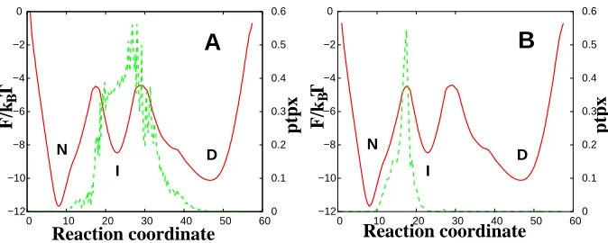
where pf old(X) = 0.5 describes an intermediate state, rather than transitions states, the criterion is not a sufficient condition of optimality and a different criteria should be used. To calculate P(T P|x) the argument ptpx should be added to command line together with the positions of the boundariesx0 and x1 and the bin size ∆x. Fig. 3 (A) shows that when the
P(T P|x) criteria applied to both transition states, it indicates that neither of the transition states are optimal. However, it shows that the first transition state is optimal, if P(T P|x) is computed just around a single TS (Fig. 3 B).
The FC,1(x,∆t)=const test of RC optimality. To test the optimality of a putative
RC for more complex systems (i.e., with more than one barrier) another criterion has been suggested recently.23The criterion assesses whether a putative reaction coordinate accurately
It states that for such a coordinate, the cut-based free energy profileFC,1(x,∆t), computed
from an ensemble of transition path segments, is x and ∆t independent.
The function testoptimality first transforms the reaction coordinate (the time series) x
to the pf old coordinate, by invoking the pfoldMSM internal function (Eq. 5). Then cut profilesFC,1 along this coordinate are constructed at different sampling time intervals ∆t=1,
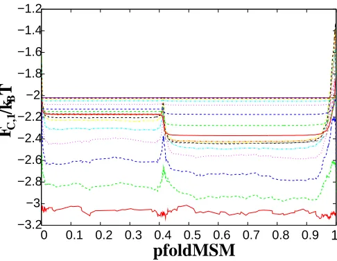
2, 4, 8, 16, ... using the transition paths.23 Fig. 4 shows cfep1 profiles constructed along
pf oldM SM(RCF IP35) with different ∆t. All the profiles are relatively parallel lines with small
fluctuations converging to the limiting profile, which means that chosen RC is close to the
pf old coordinate, however is still slightly sub-optimal.21,23
Diffusion coefficient and other quantities
Fep1d allows one to compute the diffusion coefficient according to Eq. 2 or according to Eq. 3 by adding arguments --D=1 or --D=2, correspondingly.
The mean first passage time can be estimated (a) from the trajectory by estimating the mean waiting time between the transitions and (b) with the Kramer’s equation21,29
mf pt=
∫ x1
x0
eβFH(x)/D(x)dx
∫ x1
x
e−βFH(y) dy,
where β = 1/kBT. The mean transition pass times mtpt is estimated by direct counting from trajectories. For computing these quantities the only argument --mfpt=1 should be added.
The plots of folding probability as a function of the reaction coordinate, estimated using either Eq. 4 or Eq. 5, can by obtained by using command line arguments --pfold=1 or
Conclusion
The popular approaches to analyze the results of atomistic simulations can be roughly divided into Markov state models (MSMs),31 conformation network analysis30 and the free-energy
landscape framework.2 In the former, trajectory snapshots are combined into microstates
or clusters using a variety of clustering algorithms. Construction of such a model, which accurately describes the dynamics encoded by the trajectory is a very difficult problem and a number of software packages are being developed for its solution.32,33 Once such a model
has been constructed, the properties of the dynamics are inferred by analyzing the model. In particular, one can determine the free energy basins (metastable states), transition states, pathways.2,30,31,34 The pf old optimal coordinate between any two boundary nodes can be
easily determined, and hence such properties as the cut profiles and diffusion coefficient. In particular, the popular wordom program provides such a workflow.33 In our experience,
such an approach works very well for relatively small systems (e.g., peptides with up to 15-20 residues in length).2,20,35 For larger systems, it appears that construction of a good
quality Markov state model, which accurately describes the dynamics of a system, is much more difficult due to the infamous ”curse of dimensionality”; especially in the transition state regions, where the sampling is limited. Because of that, it is difficult to determine, for example, the major properties of the folding dynamics - the folding free-energy barriers and the pre-exponential factor, the structure of the transition states (TS), the transition path times and the diffusion coefficient. The free energy profiles as functions of optimal reaction coordinates constitute an alternative framework, which allows one to determine these properties in relatively straightforward manner.
mean first passage times, the mean transition path times. However, the unique functionality of the script is the ability to assess the optimality of a putative reaction coordinate and to inspect whether the dynamics projected on such a coordinate is diffusive, rather than sub or super diffusive. Being a python script, the code can be easily read, adapted and modified to extend the functionality. We hope that it will make a rigorous analysis of increasingly available large amount of complex data less involved.
ACKNOWLEDGMENTS
The work has been supported in part by an RCUK fellowship and BBSRC grant (No. BB/J016055/1).
References
(1) Hedges, L. O.; Jack, R. L.; Garrahan, J. P.; Chandler, D.Science 2009,323, 1309–1313. (2) Krivov, S. V.; Karplus, M. Proc. Natl. Acad. Sci. USA. 2004, 101, 14766–14770. (3) Yu, H.; Gupta, A. N.; Liu, X.; Neupane, K.; Brigley, A. M.; Sosova, I.; Woodside, M. T.
Proc. Natl. Acad. Sci. USA. 2012,109, 14452–14457 .
(4) Schuetz, P.; Wuttke, R.; Schuler, B.; Caflisch, A. J. Phys. Chem. B 2010,114, 15227– 15235.
(5) Jungblut, S.; Singraber, A.; Dellago, C.Mol. Phys. 2013, 111, 3527–3533.
(6) Shaw, D. E.; Maragakis, P.; Lindorff-Larsen, K.; Piana, S.; Dror, R. O.; East-wood, M. P.; Bank, J. A.; Jumper, J. M.; Salmon, J. K.; Shan, Y.; Wriggers, W.
Science 2010, 330, 341–346.
(8) Best, R. B.; Hummer, G.Proc. Natl. Acad. Sci. USA. 2005, 102, 6732–6737. (9) Berezovska, G.; Prada-Gracia, D.; Rao, F.J. Chem. Phys. 2013, 139, 035102.
(10) Ceriotti, M.; Tribello, G. A.; Parrinello, M. Proc. Natl. Acad. Sci. USA. 2011, 108, 13023–13028.
(11) Mu, Y.; Nguyen, P. H.; Stock, G. Proteins: Structure, Function, and Bioinformatics
2005, 58, 45–52.
(12) Krivov, S. V.; Fenton, H.; Goldsmith, P. J.; Prasad, R. K.; Fisher, J.; Paci, E. PLoS Comput. Biol. 2014, 10, e1003685.
(13) Krivov, S. V. Phys. Rev. E 2011, 84, 011135.
(14) Freddolino, P. L.; Harrison, C. B.; Liu, Y.; Schulten, K.Nat. Phys. 2010,6, 751–758 . (15) Krivov, S. V. PLoS Comput. Biol. 2010, 6, e1000921.
(16) Ferguson, A. L.; Panagiotopoulos, A. Z.; Kevrekidis, I. G.; Debenedetti, P. G. Chem. Phys. Lett. 2011,509, 1–11.
(17) Rohrdanz, M. A.; Zheng, W.; Maggioni, M.; Clementi, C. J. Chem. Phys. 2011, 134, 124116.
(18) Peters, B.; Trout, B. L.J. Chem. Phys. 2006, 125, 054108.
(19) Krivov, S. V.; Karplus, M. J. Phys. Chem. B 2006, 110, 12689–12698.
(20) Krivov, S. V.; Karplus, M. Proc. Natl. Acad. Sci. USA. 2008, 105, 13841–13846 . (21) Krivov, S. V. J. Phys. Chem. B. 2011, 115, 12315–12324 .
(24) Du, R.; Pande, V. S.; Grosberg, A. Y.; Tanaka, T.; Shakhnovich, E. S.J. Chem. Phys.
1998, 108, 334–350.
(25) Darve, E.; Solomon, J.; Kia, A. Proc. Natl. Acad. Sci. USA. 2009, 106, 10884–10889. (26) Hummer, G. J. Chem. Phys. 2004,120, 516–523.
(27) Vanden-Eijnden, E.; Venturoli, M.; Ciccotti, G.; Elber, R. J. Chem. Phys. 2008, 129, 174102–174102–13.
(28) Berezhkovskii, A. M.; Szabo, A. J. Phys. Chem. B 2013, 117, 13115–13119. (29) Kramers, H. A. Physica 1940,7, 284–304.
(30) Rao, F.; Caflisch, A. J. Mol. Biol. 2004, 342, 299–306.
(31) Lane, T. J.; Bowman, G. R.; Beauchamp, K.; Voelz, V. A.; Pande, V. S.J. Am. Chem. Soc. 2011,133, 18413–18419.
(32) Beauchamp, K. A.; Bowman, G. R.; Lane, T. J.; Maibaum, L.; Haque, I. S.; Pande, V. S.
J. Chem. Theory Comput. 2011, 7, 3412–3419.
(33) Seeber, M.; Cecchini, M.; Rao, F.; Settanni, G.; Caflisch, A.Bioinformatics 2007, 23, 2625–2627.
(34) No, F.; Schtte, C.; Vanden-Eijnden, E.; Reich, L.; Weikl, T. R. Proc. Natl. Acad. Sci. USA. 2009,106, 19011–19016.
Figure captions
−14 −12 −10 −8 −6 −4 −2 0
0 10 20 30 40 50 60
F/k T
natural
B
Figure 1: Free energy profilesFC(x) (red solid line) andFH(x) (green dashed line) determined for an optimized RCF IP35 constructed for the folding trajectory of FIP35 protein using
−12 −10 −8 −6 −4 −2 0
0 10 20 30 40 50 60−0.1 0 0.1 0.2 0.3 0.4 0.5 0.6
F/k T α
natural
[image:16.612.182.430.112.309.2]B
Figure 2: FC(x) (red solid line) and α(x) (green dashed line) determined for the RCF IP35.
To calculate α(x), the command line should contain --alpha= [∆t1,∆t2]. Here, by the time
steps ∆t1 and ∆t2 we mean integer numbers referred to the steps of the trajectory: fep1d.py rc.dat --alpha=[1,8]
−12 −12 −10 −10 −8 −8 −6 −6 −4 −4 −2 −2
0 0
0 10 20 30 40 50 60 0 0 10 20 30 40 50 60 0
0.1 0.1
0.2 0.2
0.3 0.3
0.4 0.4
0.5 0.5
0.6 0.6
F/k T ptpx F/k T ptpx
Reaction coordinate Reaction coordinate
A
B
D I N D I N B BFigure 3: A) P(T P|x) calculated for theRCF IP35 (green dashed lines). The command line
is fep1d rc.dat --ptpx=1 --x0=47 --x1=8.2 --dx=1.0 with x0 and x1, corresponding to the
minima of the denatured state (D) and the native state (N); B)P(T P|x) calculated withx0
[image:16.612.137.474.473.608.2]−3.2 −3 −2.8 −2.6 −2.4 −2.2 −2 −1.8 −1.6 −1.4 −1.2
0 0.1 0.2 0.3 0.4 0.5 0.6 0.7 0.8 0.9 1
F
C,1/k T
pfoldMSM
[image:17.612.184.427.267.455.2]B
Figure 4: Testoptimality ofRCF IP35. FC,1 are shown for different sampling intervals ∆t = 1
(red line at the bottom),2, ...,216 (magenta line at the top). The command line is fep1d rc.dat --testoptimality=1 --x0=8.2 --x1=47. For function testoptimality the positions of x0