The use of time series methods in the analysis of hydrological data

(1)

THE ANALYSIS OF HYDR O L O G I C A L DATA

by

Mohan Shankar Amatya

B.Eng. (KMJ.T) , M.Eng. (Chula) Thailand

A dissertation submitted in partial

fulfilment of the requirements for the degree of

Master of Resource and Environmental Studies

in the .

Australian National University

(2)

Except where otherwise indicated, this dissertation

is my own work

M.S. Amatya

(3)

ACKNOWLEDGEMENTS

Thanks are due to Dr. A. Jakeman for guidance in the use of CAPTAIN package, to Mr M. Greenaway for helping in other programs, to Mr J. Goodspeed and Mr M. Fleming of LUR/CSIRO for allowing me to use their data on the Lerderderg Catchment area, and to Mr J.P. Brown, the District Forester of Trentham, Victoria for providing information on the fire history of the catchment area.

Helpful guidance of my supervisors Professor P.C. Young in time-series data analysis and Mr D.I. Smith in hydrology are gratefully appreciated. Finally the author is very much obliged to the Director of CRES for providing the ANU scholarship to enable him to study at CRES.

(4)

ABSTRACT

The account is based upon recursive time-series analysis and its application to the study of river catchment behaviour in order to predict future events. The Lerderderg Representative Basin, in Victoria, was selected as a range of hydrological data was available for this catchment on magnetic tape from the Land Use Research Division of CSIRO. Additional information on soil morphology and fire history was obtained from other sources.

The rainfall, runoff, evaporation and temperature records was analysed using the CAPTAIN package program and both short-term

(hourly data) and long term (daily data) were considered. Since there were no available observations for soil moisture the non-linear soil moisture compensation algorithm of CAPTAIN was used. Transfer functions and steady state gain were calculated and impulse responses analysed.

(5)

CONTENTS

Page No.

ACKNOWLEDGEMENTS ±±±

ABSTRACT iv

CONTENTS v

PREFACE V Ü

LIST OF TABLES x

LIST OF FIGURES xi

LIST OF MAPS xvii

CHAPTER 1 : ENGINEERING HYDROLOGY 1

1.1 Introduction 1

1.2 Hydrological Cycle 1

1.3 Interception 3

1.4 Ground Water 4

1.5 Evaporation 5

1.6 Transpiration 6

1.7 Infiltration 7

1.8 Overland Flow 11

1.9 Measurements in Hydrology 12

1.10 Hydrologic Systems 14

CHAPTER 2 : TIME-SERIES ANALYSIS METHODS IN HYDROLOGY 19

2.1 Unit Hydrograph 19

2.2 Unit Impulse Response 20

2.3 The Time-Series Method 25

• CHAPTER 3 :CAPTAIN CONCEPT 34

3.1 Principles 34

3.2 CAPTAIN Use 35

CHAPTER 4 :LERDERDERG RIVER CATCHMENT AREA 39

4.1 Description of the Catchment Area 39

4.2 Soil Morphology 39

4.3 Bushfire History 44

(6)

Page No.

CHAPTER 5 : TIME--SERIES MODELLING 48

5.1 Data :: Source and Type 48

5.2 Hourly Data Analysis 49

5.3 Daily Data Analysis 53

5.3.1 Analysis of Rainfall and

Data only

Runoff 54

5.3.2 Analysis of Evaporation,

and Runoff Data

Rainfall 57

5.3.3 Analysis of Temperature,

and Runoff Data

Rainfall 59

5.4 Discussion 62

CHAPTER 6 CONCLUSION 64

BIBLIOGRAPHY 67

(7)

PREFACE

Studies of hydrology have played a vital role in the development of human society over the past several thousand years. This study is aimed particularly at evaluating the relevance of system methods and particularly time-series analysis in evaluating catchment behaviour. In particular, it considers the analysis of hydrological data for the Lerderderg River basin catchment and reaches certain

conclusions on the hydrologic behaviour of the catchment on the basis of this analysis. It also attempts to evaluate the advantages and disad vantages of the time-series approach to data analysis in this particular application.

Rainfall data were collected from eight stations by the Land Use Research Division of the Commonwealth Scientific and Industrial Research Organization (LUR-CSIRO). Likewise runoff data were collected from a limited number of gauging stations. They were then processed and stored in magnetic tapes for general use. Evaporation data were collected from three stations within the catchment using class A evaporation pans. This limited data base was supplemented by the use of records from stations in neighbouring catchments in order to generalise the overall evaporation figures for the catchment. All these data and daily dry bulb temperature taken at 15.00 hrs and daily maximum temper ature were stored on magnetic tapes by LUR-CSIRO.

(8)

saturated deficit formula or maximum and minimum temperatures. Six years’ daily rainfall, runoff, evaporation, dry bulb temperature and maximum temperature data were used in this study. In addition hourly rainfall and runoff data (Glover, 1979) for short periods were also used.

The basin was assumed to be water-tight, i.e. the catchment behaviour for the purpose of this study was considered to be unaffected by the loss or gain from deep groundwater circulation originating from beyond the catchment boundary. In a strict sense, this is not accurate as some small mineral springs occur within the catchment and these are associated with deeper groundwater circulation, e.g. in the vicinity of the town of Blackwood. In other words the yield of these small springs did not effectively contribute to the overall runoff of the Lerderderg river system. In addition to these points, soil morphology and bushfire history were studied to consider their possible effects on the catchment behaviour.

A hydrological system can, in general, be either stochastic or deterministic and linear or non-linear. In this study, the determin istic linear system of rainfall-runoff was analysed first and a non linear analysis was attempted later. A new recursive approach (Young, 1972) was adopted, where estimation of the parameters in a transfer function type model were based on the recursive instrumental variable method suggested by Young and Jakeman (1979) .

As infiltration has a considerable effect on the yield of the catchment and depends upon the soil permeability, a particular form of "Antecedent Precipitation Index” (API) was considered to offset the loss due to infiltration.

Data were analysed using the computer package program

(9)

effects; to generate their impulse responses (unit hydrographs); and to approximate the standard error of the estimated transfer function parameters. The model structure identification was found to be

2 dependent on the evaluation of the coefficient of determination R^, and the error variance norm EVN (or normalised EVN, NEVN) . In order to assess the likely effects of temperature on the rainfall-runoff relationships analysis was initially undertaken for the dry bulb

temperature. The method was repeated for the maximum temperature, but as expected, there was little difference in the results.

Daily data were analysed in three ways:

(a) considering the raw rainfall only as sole input; (b) considering raw rainfall minus evaporation as the

input, and

(c) modifying the raw rainfall for temperature effects.

(10)

LIST OF TABLES

5.1 Hourly Data Sets

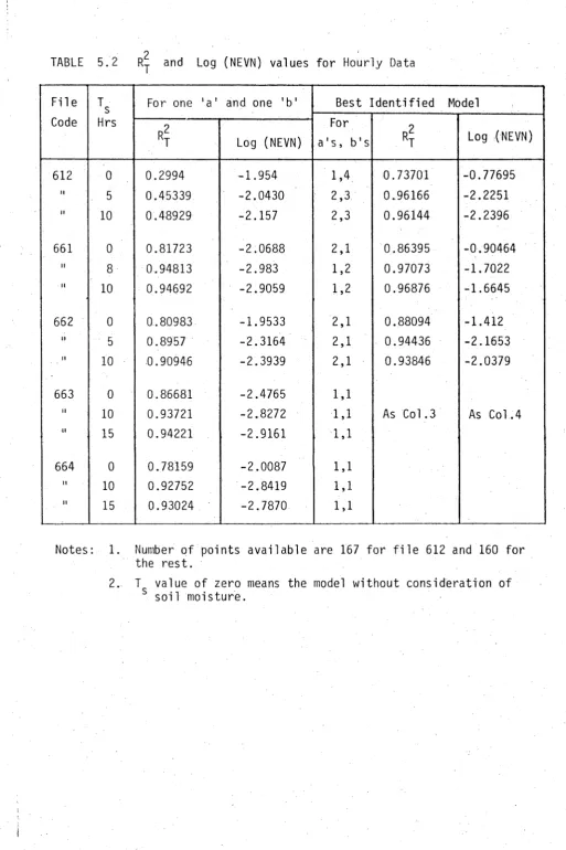
5.2 2

* T and Log (NEVN) Values for

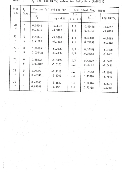
5.3 2

*1 and Log (NEVN) Values for

5.4 2

*T and Log (NEVN) Values for

5.5 2

*4

and Log (NEVN) Values for

Page N o .

50

Hourly Data (HOURLY) 51

Daily Data (RAINDIS) 55

Daily Data (SUB) 58

(11)

1.1 Systems Diagram of the Global Hydrological Cycle 2

1.2 Flow Diagram Showing Interception, Stemflow and

Throughflow 4

1.3 Infiltration Loss by <J> - index 9

1.4 The Production of Overland Flow in Response to Rainfall Intensities in Excess of the Soil

Infiltration Capacity 11

1.5 Overland Flow on Slopes 13

1.6 A Systems Representation of a Catchment Water

Balance 16

1.7 A Sequential System 17

2.1 Direct Runoff Hydrograph (75 mm), Unit Hydrograph (25 mm),

and Effective Rainfall Duration (4 hours) 21

2.2 The Linear Dynamic System 22

2.3 Rainfall-runoff Time-Series Model 25

2.4 Linear Dynamic System with Non-linear Filter 30

3.1 Recursive and Iterative Data Processing 35

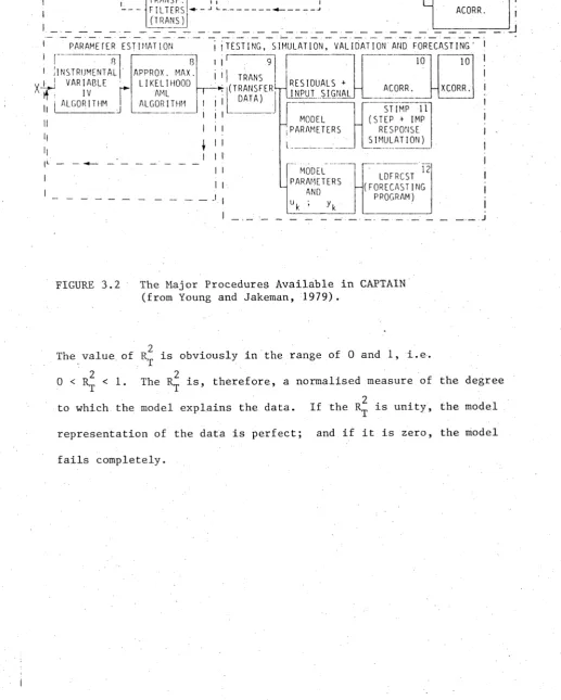
3.2 The Major Procedures Available in CAPTAIN 38

5.1 Rainfall 612 72

5.2 Rainfall 661 73

5.3 Rainfall 662 74

5.4 Rainfall 663 75

5.5 Rainfall 664 76

5.6 Runoff 612 77

5.7 Runoff 661, 662, 663 and 664 78

5.8 Raw Data Model 612 79

5.9 Model 612 with Allowance for Soil Moisture Effects 80

(T = 5 hours) s

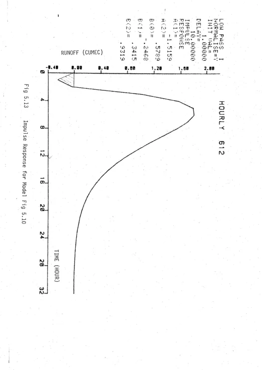
5.10 Model 612 with Allowance for Soil Moisture Effects 81

(T = 10 hours) s

5.11(a) Impulse Response for Model Fig. 5.8 82

5.11(b) Sectional Amplification of Fig. 5.11(a) 83

5.12 Impulse Response for Model Fig. 5.9 84

5.13 Impulse Response for Model Fig. 5.10 85

(12)

Page No.

(T = 8 hours) s

(T = 10 hours) s

5.17 Impulse Response for Model Fig. 5.14 89

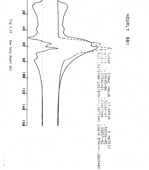
5.20 Raw Data Model 661 92

(T = 8 hours) s

(T = 10 hours) s

5.26 Raw Data Model 662 98

(T = 5 hours) s

5.28 Model 662 with Allowance for Soil Moisture Effects 100

(T = 10 hours) s

5.29 Impulse Response for Model Fig. 5.26 101

5.32 Raw Data Model 663 104

(T = 1 0 hours) s

5.34 Model 663 with Allowance for Soil MOisture Effects 106

(T = 15 hours) s

5.38 Raw Data Model 664 110

(T = 10 hours) s

(T = 15 hours) s

(13)

Page No.

5.44 Rainfall 1970 ₁₁₆

5.45 Rainfall 1971 ₁₁₇

5.46 Rainfall 1972 ₁₁₈

5.47 Rainfall 1973 ₁₁₉

5.48 Rainfall 1974 ₁₂₀

5.49 Rainfall 1975 ₁₂₁

5.50 Maximum Temperature 1970 ₁₂₂

5.51 Maximum Temperature 1971 ₁₂₃

5.52 Maximum Temperature 1972 ₁₂₄

5.53 Maximum Temperature 1973 ₁₂₅

5.54 Maximum Temperature 1974 ₁₂₆

5.55 Maximum Temperature 1975 ₁₂₇

5.56 Dry Bulb Temperature 1970 ₁₂₈

5.57 Dry Bulb Temperature 1971 ₁₂₉

5.58 Dry Bulb Temperature 1972 ₁₃₀

5.59 Dry Bulb Temperature 1973 ₁₃₁

5.60 Dry Bulb Temperature 1974 ₁₃₂

5.61 Dry Bulb Temperature 1975 ₁₃₃

5.62 Evaporation 1970 134

5.63 Evaporation 1971 ₁₃₅

5.64 Evaporation 1972 ₁₃₆

5.65 Evaporation 1973 ₁₃₇

5.68 Discharge 1970 140

5.69 Discharge 1971 141

5.70 Discharge 1972 142

5.71 Discharge 1973 ₁₄₃

5.72 Discharge 1974 144

5.73 Discharge 1975 145

5.74 Raw Data Model Raindis 70 146

(14)

Page N o .

5.81 Impulse Response for Model Fig. 5.75 1 5 3

5.86 Model Raindis 70 with Allowance for Soil Moisture 158

5.98 1970 Model Response with Parameter Values Set to 170

those Estimated for 1971 (Fig. 5.87)

5.103 Modified Input SUB 70 175

5.109 Model for Modified Input and Measured Runoff 1970 181

5.110 Model for Modified Input and Measured Runoff 1971 182

(15)

P a g e N o .

5 . 1 1 2 M o d e l f o r M o d i f i e d I n p u t a n d M e a s u r e d R u n o f f 1 9 7 3 1 8 4

5 . 1 1 3 M o d e l f o r M o d i f i e d I n p u t a n d M e a s u r e d R u n o f f 1 9 7 4 _{1 8 5}

5 . 1 1 4 M o d e l f o r M o d i f i e d I n p u t a n d M e a s u r e d R u n o f f 1 9 7 5 1 8 6

5 . 1 1 5 I m p u l s e R e s p o n s e f o r M o d e l F i g . 5 . 1 0 9 1 8 7

5 . 1 2 1 M o d e l F i g . 5 . 1 0 9 A l l o w i n g o f 5 d a y s 1 9 3

5 . 1 2 3 M o d e l F i g . 5 . 1 1 1 A l l o w i n g T g o f 5 d a y s 1 9 5

5 . 1 2 5 M o d e l F i g . 5 . 1 1 3 A l l o w i n g T o f 5 d a y s

s 1 9 7

5 . 1 2 6 M o d e l F i g . 5 . 1 1 4 A l l o w i n g T g o f 5 d a y s 1 9 8

5 . 1 3 3 1 9 7 0 M o d e l R e s p o n s e w i t h P a r a m e t e r V a l u e s S e t t o

E s t i m a t e d f o r 1 9 7 1 ( F i g . 5 . 1 2 2 )

t h o s e 2 0 5

t h o s e 2 0 6

t h o s e 2 0 7

t h o s e 2 0 8

t h o s e 2 0 9

5 . 1 3 8 1 9 7 0 R a i n f a l l M o d i f i e d b y D r y - b u l b T e m p e r a t u r e 2 1 0

5 . 1 3 9 1 9 7 1 R a i n f a l l M o d i f i e d b y D r y - b u l b T e m p e r a t u r e « 2 1 1

5. 1 4 2 1 9 7 4 R a i n f a l l M o d i f i e d b y D r y - b u l b T e m p e r a t u r e 2 1 4

(16)

5.144 5.145 5.146 5.147 5.148 5.149 5.150 5.151 5.152 5.153 5.154 5.155 5.156 5.157 5.158 5.159 5.160 5.161 5.162 5.163 5.164 5.165 5.166 5.167 5.168 5.169 5.170 5.171

Page N o .

1970 Model Allowing for Temperature (dry bulb) 216

Effects

Impulse Response for Model Fig. 5.150 222

Impulse Response for Model Fig. 5.151 223

Model Fig. 5.150 Allowing for Soil Moisture Effects 228

1970 Model Response with Parameter Values Set to those 240

Estimated for 1971 (Fig. 5.163)

(17)

LIST OF MAPS

Page N o .

1. Lerderderg River 40

2. The Lerderderg River Catchment Basin 41

3. The Lerderderg River System 42

(18)

ENGINEERING HYDROLOGY

1.1 Introduction

Hydrology is the branch of science that deals with the

occurence, distribution and movement of water on, over and under the surface of the earth (Ward, 1975). It has been defined in numerous ways, one of the most comprehensive being 'the science of the world's waters, the different forms in which they exist' (Batisse, 1964). There are four basic processes in hydrology viz. precipitation, evap oration and transpiration, surface runoff and groundwater flow.

The scope of hydrology is extremely wide. It is closely linked with a number of other environmental sciences such as

geomorphology, climatology and ecology (Rodda, Downing and Law, 1976). Engineering hydrology is concerned with various methods of controlling the use of water and, in particular, the amount of rainfall, the length of dry period, the amount of storage, losses due to evapotranspiration in river basin or catchment, the regulations of surface runoff, and the design, plan and construction of storage reservoirs and irrigation canals (Wilson, 1974).

1.2 Hydrological Cycle

The movement of water from the sea to the atmosphere and then by precipitation to the earth, where it collects as runoff and returns

(19)

structures. Besides that, there is no uniformity in the time a cycle takes. The intensity and frequency of the cycle depend on a variety of geographical and climatological factors. The various parts of the cycle can be complex in detail and a hydrologist can have some control only on the land-phase of the cycle (Wilson, 1974). Figure 1.1 shows the system diagram of the global hydrological cycle.

( m ) o v o p o t r o n s p i r a t i o n

( i ) t r a n s p i r a t i o n

( e ) p r e c i p i t a t i o n —

t o ) i n t e r c e p t i o n

( b ) s 1 e rr. f I o w a n d t h r c u g h f c l l

( f ) o v e r l a n d f l o w f l o o d s —

c a p i l l a r y i n f i l t r a t i o n

( g ) i n t e r f l o w

p e r c o l a t i o n

--- ( h ) b o s e f l o w

---( t ) r u n o u t

6 OCFAN BASINS

( j ) e v a p o r a t i o n

2 SURFACE

3 SOIL MOISTURE 1 VEC STATION

U . GROUND

WATER 7. ATMOSPHERE

(20)

The sea-water evaporates due to solar radiation and moves over land areas as water vapour which is precipitated in the form of snow, hail and rain. Part of such precipitation infiltrates into the soil and moves down into the saturated ground zone beneath the water-table. This phreatic zone is usually connected by aquifers to river systems or

to the sea. Part of the infiltrated water is transpired from leafy plants of the vegetated surfaces. Further precipitation is intercepted by the branches and foliage of plants. This is known as interception and may take three possible routes. If the water drips off the plant leaves to ground, the process is known as throughfall. If there is another interception to that, it is known as secondary interception. On the other hand, the water may run along the leaves, branches and then stems to reach the ground. This is referred to as stemflow. Part of the water intercepted may return to the atmosphere by evaporation. These processes are shown in Figure 1.2. Part of the surface water returns to the atmosphere by evaporation and the rest form the river systems which again lose a certain amount through evaporation. Another part of the cycle, ground water, moves slowly to join the river systems to return to the sea.

1.3 Interception

Interception loss varies with the duration and intensity of the precipitation. It also varies over time as a result of seasonal

variations in the vegetation (Weyman, 1975). Penman (1963) showed that there was a fivefold increase in summer interception under a cover of cereal crops compared to the winter equivalent. There are also spatial variations in interception loss due to various plant species. Lull

(21)

Secondary throu gh fa ll Rainfall

Secondary interception by gro un d flora Total eva po ration

loss from toliaqe

Proportion of total rainfal reaching the soil

FIGURE 1.2 Flow Diagram Showing Interception Stem!low and Throughflow (from Smith and Stopp, 1978).

throughfall and stemflow. Although the interception has considerable

effect upon the reduction of gross precipitation to net precipitation, no rigorous method has been found for the estimation of interception

loss.

1.4 Ground Water

Any phenomenon which produces a change in pressure on the

ground water causes the ground water level to change. Changes in

storage, resulting from differences between recharge and discharge of

water, cause levels to vary in time from a few minutes to many years.

Variations of runoff stages and evaporation produce localised storage

changes. Secular variations in levels extending over periods of

(22)

in which rainfall is above or below the mean. Though recharge is the governing factor of ground water level depending on the rainfall intensity and distribution and the amount of surface runoff, rainfall is not an accurate indicator of groundwater level changes (Todd, 1964). A certain degree of control on ground water levels is possible, for example the regulation of seepage through earth dams and land drainage

(Todd, 1959).

The main concern of hydrologists is the detailed quantitative study of water occurence distribution and movement, i.e. precipitation, evapotranspiration, surface runoff, and ground water flow in a specific area, to predict the most likely quantities involved in the extreme cases of flood and drought, and also the likely frequency with which such events will occur, since such a frequency is a very important part of the hydraulic engineering design (Wilson, 1974).

The hydrology of a specific area or a catchment depends on its topography, geology and climate. The important climatic factors like precipitation, humidity, temperature, and winds have strong effects on the process of evapotranspiration. Precipitation and various

storage of water and high and low rates of runoff are highly influenced by the topography. Geology is another important factor because it influences the topography and because the groundwater zone is where the catchment's underlying rock lie.

1.5 Evaporation

(23)

and reflective properties of the surface (the albedo) and differs for various surfaces exposed to or shaded from solar radiation. Solar radiation, wind, relative humidity and temperature are the main factors affecting evaporation. The process of evaporation is most active under the direct radiation of the sun since the process is endothermic. During the process of vaporisation of water the boundary between the earth and air becomes saturated. For the evaporation to continue, the saturated boundary must be replaced by drier air. As the humidity rises, its ability to absorb more water vapour decreases and evaporation slows down. So, unless the boundary layer of the saturated air is replaced by drier one, the evaporation rate will decrease. If the ambient temperature of the air and ground is high, evaporation will take place more rapidly than if they were cool. Since the capacity of air to absorb water vapour increases with the increase in its temperature, the air temperature has a double effect on the

process of evaporation. Recent developments in the study of evaporation can be found elsewhere (e.g. Webb, 1975 and Hoy and Stephens, 1979).

1.6 Transpiration

A small portion of the water required for a plant is retained in the plant structure. Transpiration is the process by which water vapour escapes from the living plant, particularly the leaves, and enters the atmosphere (Ward, 1975). In the case of ground covered with vegetation, it is very difficult to differentiate between

(24)

close up and very little moisture leaves the plant surfaces. On the other hand evaporation continues so long as heat input is available and, of course, basically during the day time. Penman (1948)

established, for the estimation of evapotranspiration, the first and most complete theoretical relationship which shows that the evapo

transpiration is inseparably connected to the amount of radiative energy gained by the surface. This relationship has been widely used in Britain, Australia and the eastern part of the U.S.A. (Veihmeyer, 1964). Further development has been reported elsewhere (e.g. Penman, 1970 and Denmead, 1973).

1.7 Infiltration

In the case of the surface being completely wet, the subsequent rain must either penetrate the surface layers or run off the surface to meet a river system. Runoff or penetration depends upon the permeability of the surface. Vegetated areas are always permeable to some degree. Infiltration, therefore, takes place in all the vegetated areas. Once the infiltrating water passes through the surface layers, it then percolates downwards until it reaches the zone of saturation at the phreatic surface. The infiltration rate varies with the type of soil and is the sum of percolation and water entering storage above the ground-water table.

Horton (1945) established the first relationship for the infiltration rate as:

where

f + p e-kt

f - infiltration rate at any time t (mm/h)

(25)

f = infiltration capacity at large value of t(mm/h) c

f = initial infiltration capacity at t = 0 (mm/h) o

t = time from beginning of rainfall (min)

k = constant for a particular soil and surface (min *) (e.g. larger value for smoother surface texture like bare soil, and smaller for vegetated surface)

A number of formulae have been proposed since then but further details can be found elsewhere (e.g. Wilson, 1974; Ward, 1975).

Approximations of infiltration losses can be made by means of infiltration indices (Wilson, 1974) . One of them is the <}>-index which is the average rainfall intensity above which the volume of rainfall equals the volume of runoff. In Figure 1.3 the unshaded area below the line represents the amount of rainfall that is not accounted as a part of runoff but as losses including surface detention, evaporation, and infiltration. This cannot be used in predicting the amount of

rainfall being absorbed by the soil, because this is dependent on the state of wetness of the soil at the beginning of the rain. As the infiltration is much the largest loss in many catchments, and the infiltration capacity as well as the amount of run-off depends on the initial soil moisture, forecasting runoff is not simple.

To overcome this difficulty, to a certain degree, an

(26)

ne! r a n = ) quo nt'ty of

ru nnf f

$ index

'■ me in h o u r s ---

*-FIGURE 1.3 Infiltration Loss by <{)-index (from Wilson, 1974)

To predict the catchment behaviour and its response to storms, it is necessary to analyse input and output of the catchment. Such analyses can be carried out with the help of ’black-box’ model which will be described, in detail, later. This model establishes a relation ship between total storm rainfall and total storm runoff. The validity of the relationship, however, is limited because the runoff does not vary with the rainfall alone but depends on other factors viz. intensity and duration of the rainfall and, more important, antecedent catchment moisture. At early stages of the hydrological development, the base-

flow discharge was used as an indication of catchment storage at the start of a storm. One of the earliest methods to forecast direct runoff volumes was the co-axial graphical correlation method of Linsley et aZ.

(27)

day in question (Weyman, 1975). Thus the A.P.I. calculated on the basis of n days preceding rainfall is written as:

n -t

A.P.I. = £ P .k n t=0 1

where P^_: the precipitation on a day t before the calculation date, and k : constant.

Runoff can be predicted, by using multiple regression analysis, from the combined effect of rainfall and A.P.I. Weyman (1975) has given a good numerical example. The procedures used in the present study are similar to this but have a sounder grounding in systems and estimation theory.

Using a somewhat more detailed level of analysis, Body (1975) expressed that, under Australian conditions, there could be a significant portion of the early storm rainfall totally lost to runoff. This

assumption of loss effect necessitated the introduction of a gross approximation of the water balance for a catchment. The initial loss may be correlated with an indication of catchment moisture status

(e.g. A.P.I.), while the <£-index can be related to the duration of the excess rainfall. Body (1975) argues that these approximate methods are sufficiently accurate in larger size catchments for two reasons:

1. The considerable storage available damps out short period responses to more intense rainfalls over limited areas, and the

catchment contributes runoff only after initial infiltration capacities have been reduced over a significant proportion of the area.

2. The significance of spatial variation in the soil moisture content is reduced by the averaging effect caused by the extent of the area involved, in much the same way as the significance of rainfall variability is reduced when real rainfall estimates are considered.

(28)

1.8 Overland Flow

It is generally accepted that the overland flow is the result of rainfall intensities in excess of the infiltration capacity of the

soil (Horton, 1945). Figure 1.4 illustrates an infiltration curve superimposed upon the histogram of storm rainfall, where the shaded area indicates the volume of water left on the ground surface. During the course of a storm, the portion of precipitation left over the surface increases, when the infiltration capacity decreases. On flat areas, or those with very low gradients, soil infiltration capacity is exceeded over the entire area of one soil type more or less simultane ously before overland flow is observed. But on slopes, where overland flow is observed, measured infiltration rates are frequently very high. The term 'overland flow' is used for flow physically over the hillslope surface, and 'runoff' is only for streamflows and not associated with any particular hillslope flow component (Carson, 1972). When overland flow occurs on slopes with a high infiltration capacity, surface water is restricted to only part of the slope. The infiltration-excess

overland flow may, therefore, be restricted to the special cases of the clay soils or soils suffering from surface compaction (Weyman, 1975).

Infiltration rate

Rainfall in excess of infiltration

Rainfall lost to infiltration

Time since start of rainfall (hours)

(29)

Numerous assumptions have been made on the way precipitation

reaches river systems from hillslope areas. Figure 1.5 illustrates the

Horton (1945) Overland Flow and Saturated Overland Flow. Movement of

runoff over the land surface is overland flow, whereas downslope

movement within the soil profile is termed throughflow or interflow

and the slower movement through the bedrock is baseflow. The flow

seeping through bedrock is termed groundwater flow. These routes

basically depend on various factors such as rock permeability, soil

texture and depth, and rainfall intensity of the catchment under study.

During the process of vertical infiltration, water can enter saturated

soil into underlying unsaturated soil. However, if surface saturation

is maintained by throughflow from upslope, further precipitation may not be able to enter the soil.

Weyman (1975) argues that the measurement of infiltration

capacity under normal conditions does not reveal this characteristic,

and the control or saturated overland flow is the pattern of soil

moisture existing at the start of a storm or developed during the storm.

The water following different routes accumulates in hollows and at the

base of hillslopes before it moves laterally to join a river system.

Other details of these processes can be found elsewhere (e.g. Ward, 1975) .

1.9 Measurements in Hydrology

Runoff is generally measured in cubic meters per second, cumecs.

There are various methods used to measure it and they fall into three

categories, namely the dye dilution methods, velocity and cross-sectional area method, and methods involving the use of control structures like

(30)

Ri ver

-rp

o

0 & o

..

**. . * . ’6 ° * o c ° o °**

>V " O0 0 o A 0fü ° c

.•0o o o o o o V < 0 o

°

0

(a)

Rainfall i n t e n s i t y more than

i n f i l t r a t i o n capacity.

Ri ver

(b)

Rainfall i n t e n s i t y not neces s ar i l y more than i n f i l t r a t i o n capacity.

(31)

and in millimeters. Evaporation is directly measured from the free

water surface of evaporation pans and in millimetres. But transpira

tion, being essentially a botanical process, is difficult to measure;

direct measurement of evapotranspiration is virtually impossible. The

normal practice is to take the measurement of potential evapotranspira

tion, which is the amount of water loss that would occur if sufficient

moisture were always available for the needs of the vegetation that

covers the area, and from which an actual evapotranspiration is estimated

(Smith and Stopp, 1978).

Infiltration capacity of a soil-cover and soil moisture complex

is determined in two ways. One is the analysis of hydrographs of runoff

from natural rainfall on plots and watersheds; the other is the use of

infiltrometers with artificial application of water to enclosed sample

areas. However, both are subject to some error (Musgrave and Holtan, 1964).

1.10 Hydrologic Systems

Every hydraulic project requires a prior knowledge of the

catchment behaviour and responses, particularly the exact magnitude

and actual time of occurence of all streamflow events and their

variations in the catchment. Where full details of this type are

not available, various assumptions are necessary in order to derive

sensible hypotheses on the hydrological system behaviour which can be

tested against the available measurements. This problem has dominated

engineering hydrologists' attempts to simplify complex hydrologic

systems and to construct appropriate models for the prediction of the

catchment responses to various natural and man-made hydraulic phenomena.

(32)

that the historic hydrology of the catchment, as observed over some time, will be repeated either completely or in part. One outcome of this principle is the mass-curve of runoff analysis (Linsley, Kohler and Paulhus, 1958) which is widely used for the determination of storage yield. Further development necessitated the consideration of water balance of catchments. For small areas, Slatyer's (1967) water balance relationship over a time t is:

P - 0 - U - E + A W = 0 where P : precipitation

0 : runoff

U : deep drainage

E : evapotranspiration and A W : change in soil water storage

since a catchment is of large area, this relationship has been modified (Rodda, Downing and Law, 1976) to the form,

P = R + E + A W

where P : mean catchment precipitation R : mean catchment run-off

E : mean catchment actual evapotranspiration A W : mean storage change over the catchment

(33)

Outgoing

water

vapour Incom ing

w a te r

vapour

Evaporation and

transpiration

I n t e r f lo w S u ' f o c e d e ' e n t i o n

A t m O S P ^ e n C we l t e r

Deep percolation

S im p lifie d ca tc h m e n t m odel

FIGURE 1.6 A Systems Representation of a Catchment Water Balance (from Rodda et al.> 1976).

A system has been defined in many ways. One of them is an aggregation or assemblage of objects united by some form of regular interaction or independence (Chow, 1964a) . A system is dynamic if there is a temporally important process taking place in it and is stochastic if the process can only be described, at least in part, in probabilistic terms. As the representation of stochastic system is rather complex most of the hydrologic system models used up to the present have been treated in purely deterministic terms. If, in a system, the

(34)

law of probability, the process is known to be deterministic, otherwise stochastic. A detailed analysis of stochastic processes has been given by Papoulis (1965) and Box and Jenkins (1970). And the stochastic system approach has been extensively used by Whitehead, Young and Hornberger (1979) in the Bedford-Ouse River study.

If the system consists of input, output and some working fluid (matter, energy or information) known as throughput passing through the system, it is known as sequential system (Chow, 1964a). Figure 1.7 shows a sequential system representation. A system in a real world is a

physical system. So the hydrological cycle is a physical, sequential and dynamic system which operates within a set of constraints or physical laws that control the movement, storage, and disposition of water within the system and which derives its energy from the spatial imbalances between incoming and outgoing radiation (Freeze and Harlan, 1969). A system is said to be linear if none of its terms involves powers or products of the output, and non-linear if it produces an output which does not bear a simple algebraic relation to the components of its inputs (Bennett and Chorley, 1978). In the linear system, the transfer function remains constant for all magnitudes of input, whereas in non linear one, the transfer function becomes a function of the magnitude of the input.

(35)

In the present study, deterministic linear system of rainfall- runoff model is first analysed for the Lerderderg River basin catchment and because of the differences of this type of model, a non-linear system approach is attempted later. The study is carried out to analyse the catchment behaviour of the Lerderderg River basin on the basis of both daily data, as well as short period hourly data.

All analysis is based on time-series methodology using the CAPTAIN

(36)

CHAPTER 2

TIME-SERIES ANALYSIS METHODS IN HYDROLOGY

2.1 Unit Hydrograph

A hydrograph is a plot of stage, discharge, velocity or other properties of surface runoff with respect to time (Chow, 1964a). Both

the quantity and intensity of the rainfall have a direct effect on the hydrograph. A unit hydrograph approach is normally made to study the distribution of direct runoff volume in time. This technique was first suggested by Sherman (1932). Sherman’s approach is that, since a

surface runoff hydrograph describes many of the physical characteristics of the catchment area, similar hydrographs will be produced by similar rainfalls occuring with comparable antecedent conditions. So, if the unit hydrograph for a particular catchment and a particular duration of rainfall is known, then the runoff from any other rainfall of any

duration or intensity may be predicted, in which case a unit hydrograph functions like an impulse response of a linear system.

A unit hydrograph is the hydrograph of a unit volume of direct runoff from the entire catchment area resulting from a short, uniform rainfall (usually one inch) with an excess of unit duration (Ward, 1975) There are three hypotheses involved with the establishment of the

correlation between the effective rainfall (i.e. the rain remaining as runoff after all losses by evaporation, interception and infiltration have been considered) and the surface runoff (i.e. the hydrograph of runoff minus baseflow) (Wilson, 1974):

(37)

2. For a particular catchment and for an effective rainfall of uniform

intensity, different intensities of rainfall of the same duration

yield runoff hydrographs whose ordinates, at any given time, are

in the same proportion to each other as the rainfall intensities.

3. The principle of superposition applies to hydrographs resulting from

contiguous and/or isolated periods of uniform intensity effective

rai n .

recorded hydrograph of a uniform isolated storm with a fairly large

volume of runoff and having separated out the baseflow by dividing the

discharge ordinates of the remaining direct runoff hydrograph according

to the volume under the hydrograph, i.e. the hydrograph of 1 inch

(or 25 mm). Figure 2.1 illustrates one where the direct runoff hydro

graph representing a runoff volume of 75 mm has been divided by 3 to

yield a unit hydrograph (Ward, 1975). Since the unit storm in this

figure is of four hours duration, the derived unit hydrograph is

referred to as a 4-hour unit hydrograph.

2.2 Unit Impulse Response

A basic result in Laplace transform theory (Sneddon, 1972 and

Bracewell, 1978) concerns the relationship between two time functions

f^(t) and f^(t). If fj^(t) and f^(t) ate Laplace transformable and have

the transforms F^(s) and F 2 (s) respectively, then the product of F^(s)

and F 0 (s) is the Laplace transform of f(t) which results from the

convolution of f^(t) and f ^ t ) ,

Conventionally a unit hydrograph is generally obtained from a

f(t) [F^s) F2(s)]

(38)

Rai nf al l e x c e s s

D i r e c t r u n o f f

Unit h y d r o g r a p h

(25 m m )

Time (hours)

FIGURE 2.1 Direct Runoff Hydrograph (75 mm), Unit Hydrograph (25 mm), and Effective Rainfall Duration (4 hours) - (from Ward, 1975)

= /q f2(t—t) f2 (x) dx (2.2)

where x is a dummy variable for t and L ^ denotes inverse Laplace transform.

Now for an ordinary linear dynamic system, if all initial

conditions in the system are zero, as in the case of an isolated storm, then the input and output transforms are related by an equation:

V (s) = H (s) V.(s) (2.3)

where

H(s) : transfer function or system function, V^(s): input transform, and

(39)

V i (s)

V s

)

FIGURE 2.2 The Linear Dynamic System

Since Vq(s) in Equation (2.3) is the product of transforms, the convolution integral can be applied as:

v (t) = L 1 [H (s) V.(s)] = v .(t) h(t-x) dx (2.4)

o l U l

= /*: v.(t-x) h(x) dx (2.3)

0 l

These Equations (2.4) and (2.5) are similar to Equations (2.1)

and (2.2). Now, if v (t) = 6(t), the unit impulse or delta function, then

the transform of the unit impulse is V^(s) = 1. Under this condition, Vq(s) = H(s) or v^(t) = h(t) is the impulse response of the system and

the inverse transform of the transfer function H(s) as well. The impulse

response is thus another characteristic of the system just in the way the transfer function is. The Equations (2.4) and (2.5) suggest that if h(t),

the impulse response, is known, then only the input V (t) is to be known

in order to determine the output through the convolution operation. That

is to say that any input convolved with the unit impulse response yields

the output.

Such unit impulse response is known as the weighting function of

the corresponding linear system (Davenport and Root, 1958). Although the

present output is determined by all past history of the input weighted by

the impulse response, the output at any time is mainly determined by

recent values of the transient input and output (Panter, 1965,

Van Valkenberg, 1974). This is one good method of studying the form

(40)

linear system may be described by exciting the system with an impulse function and measuring the output (impulse) response (Kuo, 1962). This method is applicable only to ’linear shift invariant systems’ and

provides the information on the system needed to calculate an output corresponding to a given input. But it does not necessarily provide any understanding of the internal functioning of the system (Champeney,

1973).

All mathematical models of dynamic systems are characterised by three components (Faurre and Depeyrot, 1977):

(i) time;

(ii) input quantities provide the major mechanism controlling perturbations in the system, and

(iii) output quantities show the results of the system behaviour.

As a result the mathematical model of a dynamic system can be obtained from the statistical analysis of time-series data. This is particularly necessary when stochastic disturbances offset the system and distort the

observed input-output behaviour. Such time-series models can be expressed in linear differential or difference equations.

There are two approaches to evaluating the dynamic behaviour of stochastic systems of linear differential or difference equation type.

1. Mechanistic Approach: here the transformation of the input into the output is indirectly represented by introducing the notion of the state of the dynamic system (Beck and Young, 1975). The approach is based on the estimation of parameters in a model obtained by the

analysis of both the internal mechanisms, i.e. the state equation, that governs the system operation and its external signal topology (Young,

(41)

the output of the system when overall past history of the input is

known. Two examples are intuitive macro-modelling of a socio-economic

system, and predicting the behaviour of an automobile from its entire

history and all past trips. Therefore, a state of a dynamic system is

a set of quantities summarising the past in order to study the future

(Faurre and Depeyrot, 1977).

2. Input-output or 'Black-box Approach': this approach utilises the

external description of the dynamic system. The overall input-output

relationship of the dynamic system is inferred directly from the observed

input-output data. According to Eykhoff (1974), this approach is not

always very realistic, although experimenters in many cases have derived

some physical insight into the system model under consideration by extend

ing the analysis to incorporate a priori knowledge. This may provide

some information on the system, making the box more or less 'grey' or

translucent.

The mechanistic approach can provide valuable information on the

system functioning of the model. On the other hand, despite its

limitations, the 'black-box' approach is simple in terms of its inherent

parametric efficiency (i.e. the model is characterised by very few

parameters). No matter how limited the information this approach

provides on the internal system functioning, it offers a very useful

basis for both assessing input-output behaviour and forecasting future

behaviour of the output variable (Box and Jenkins, 1970).

Young (1972) has suggested a new recursive approach to the

classical procedures of time-series analysis which allows for the

estimation of parameters in linear as well as non-stationary dynamic systems which are subject to both deterministic inputs and stochastic

(42)

approach to the alternative non-recursive maximum likelihood methods of

Box and Jenkins (1970). For example, the recursive approach provides

greater flexibility and on-line potential though, in its simplest form (see next chapter), it lacks some of the desirable statistical properties

of the en-bloc methods. Before describing this recursive approach

to time-series analysis, however, it is necessary to consider the nature of time-series models and their relationship to more conventional

hydrological models.

2.3 The Time-Series Model

In a time-series model, the estimation of parameters is usually considered in a discrete time-series or pulse (3) transform transfer function representation of a linear stochastic dynamic system, as shown in Figure 2.3.

Linear Process

Input Output

(Rainfall) (Runoff)

FIGURE 2.3 Rainfall-runoff Time-Series Model

In this model, the output of the system, y , is related to two inputs:

K.

deterministic and measurable input, u , and the disturbances, £ . This

K. K.

noise input is completely uncorrelated with the deterministic input, u . k

In this study the output of the system, y is measured runoff flow while

K.

(43)

6 , i s t o c o n s i d e r a n y u n c e r t a i n t y a r i s i n g i n t h e o v e r a l l s y s t e m b e c a u s e K.

i t i s e x t r e m e l y d i f f i c u l t t o e x p l a i n t h e r e a l w o r l d i n c o m p l e t e l y

d e t e r m i n i s t i c t e r m s .

T h e o b s e r v a t i o n o f h y p o t h e t i c a l n o i s e - f r e e r u n o f f , x , a t t h e

K.

k t h i n s t a n t i s r e l a t e d t o t h e p a s t v a l u e s x, , , x. , x, a n d

r k - l k - 2 k - n

t o t h e p r e s e n t an d p a s t v a l u e s o f t h e r a i n f a l l i n p u t u ^ b y t h e d i s c r e t e

m o d e l ( Y o u n g , 1 9 7 2 ) :

\ + a i

\ - i + + a n x, k - n b o k u. + . . . + b n u, k - n (2.6)

T h e o u t p u t o f t h e w h o l e s y s t e m , t h e n , b e c o m e s

yk = xk + 'T

( 2 . 7 )

R e a r r a n g i n g E q u a t i o n ( 2 . 7 ) a s x ^ = y ^ - a n d s u b s t i t u t i n g t h i s i n

E q u a t i o n ( 2 . 6 ) , t h e d i s c r e t e r e l a t i o n s h i p b e t w e e n t h e e s t i m a t e d r u n o f f

a n d m e a s u r e d r a i n f a l l b e c o m e s :

yk + a l y k - l + • • • + 3 n y k - n = b o \ + • ' • + bn V n + \ ( 2 ' 8)

w h e r e t h e s t o c h a s t i c p a r t o f t h e s y s t e m i s

n. = t + a t . + . . . + a 6,

k k 1 k - l n k - n ( 2 . 9 )

w h i c h a r e s e r i a l l y c o r r e l a t e d b o t h i n t i m e a n d w i t h y ^ , i = k , . . . , k - n .

E q u a t i o n ( 2 . 8 ) c a n now b e e x p r e s s e d i n v e c t o r f o r m a s :

\ ± + \ (2.10)

w h e r e

an d

gk = ( - yk - l ’ • • • ’ - yk-n> uk ’ • • • ’ V n

(44)

From Figure. 2.3, we see that the deterministic part of the

system is expressed by the difference equation:

a[z 1 1 = B[z 1 ] u^

B[Z X ]

A[Z

^TT uk

]

G[Z_1 ] u,

(

2

.

11

)

where the operational notation Z ^ is the backward shift operator,

e.g. Z " 1 x k = xk _ L , and

A [ Z _ 1 ] = 1 + a. Z_1 + ... + a Z~n

1 n

B[Z 1 ] = b + b. Z 1 + . . . 4- b Z n

o 1 n

Hence, from Equations (2.7) and (2.11)

B [ Z-1

h = ---- T- Ui +

k AtZ"1] k k

(

2

.

12

)

B[Z h

where ---- :— is the transfer function of the system which is normally

A[Z~ j

assumed to be stable, i.e. the roots of the polynomial A[Z ] lie outside

the unit circle in the complex plane (Young, 1972).

Alternatively the Equation (2.12) can be written as

yk = G[Z_1] uk + Ck (2.13)

where the polynomial G[Z ] is nominally infinite dimensional, as obtained

by the division of B[Z ^ ] by A[z M , and is expressed as

G[z h = g0 + gj Z 1 + ... + gm z m + ... + g„ z (2.14)

Therefore Equation (2.13) becomes

y, = g U, + g. U, ! + . . . + g u. + E,.

(45)

This equation gives an expression for the impulse response or weighting sequence model, in which the output flow of time k is nominally given by the weighted sum of all past values of rainfall and the noise term ^

(Whitehead, Young, Hornberger, 1979). For the pure deterministic case, where u^ = p^o’ t^1G resPonse> y^> to the unit impulse, u^, is given

by yk = Sk ’ where k=0, * • • » 00

It is now clear that Equation (2.15) is directly equivalent to the unit hydrograph representation. For the purpose of the present study,

therefore, the unit impulse u is equivalent to a unit storm disturbance K.

and the infinite dimensional unit hydrograph model can be alternatively represented by the finite dimensional transfer function model Equation

(2.11),

bn + b . Z + ... + b Z

0 1 n

1 + a . Z + ... + a Z

1 n

u k

1 ^ n 1. ii

x, = -a,Z x, —a Z x, - ... -a Z x.+b^u+b.Z u. + ... +b Z u,

k 1 k 2 k n k O k l k n k

Eliminating backward shift operators, x is given by K.

X = - a x . - a x ... - a x +b u +b u , + b u + ... +b u (2.16) k 1 k-1 2 k-2 n k-n O k 1 k-1 2 k-2 n k-n

Thus, for example, the impulse response of the deterministic system for various observation instants, k ’s is given by

when k=1

x i = b .0 1 = b o

k=2

x 2 ~ -aixi+ bj

k=3

x3 = -3lx 2 - a

1 1 1

1 2 2 1 2

etc.

For other inputs, the calculation is similar provided the history of the input sequence is defined over all k. These calculations are ideally

(46)

As will be seen in later chapters, the model equation (2.12) characterises the rainfall-runoff data, and the impulse response

obtained by estimating the A[Z ^] and B[Z ^] polynomials provides the unit hydrograph resulting from the direct run-off. Since instrumental variable methods of estimation are used in the time-series analysis, a prior base flow separation is not required in such analysis. In the short term response considered predominantly in rainfall-runoff analysis, the base flow can be considered as not correlated with the rainfall input. Consequently it is also not correlated with the "instrumental variables" used in the analyses. As a result, the terms involving base-flow in the estimation equations approaches to zero, i.e.

P lim

f

k-x» k k 0

where the instrumental variable;

that part of the flow which constitutes the base-flow.

In other words, the base-flow is considered as additive noise for the purpose of estimation; so that the resulting model accounts only for

the direct runoff effect of rainfall. In a real case, if the rainfall