rsta.royalsocietypublishing.org
Research
Cite this article:Neild SA, Champneys AR, Wagg DJ, Hill TL, Cammarano A. 2015 The use of normal forms for analysing nonlinear
mechanical vibrations.Phil. Trans. R. Soc. A
373: 20140404.
http://dx.doi.org/10.1098/rsta.2014.0404
Accepted: 23 June 2015
One contribution of 11 to a theme issue ‘A field guide to nonlinearity in structural dynamics’.
Subject Areas:
structural engineering, mechanical engineering
Keywords:
nonlinear dynamics, normal forms, modal analysis, cable vibration
Author for correspondence: Simon A. Neild
e-mail:[email protected]
†Present address: School of Engineering,
University of Glasgow, Glasgow, G12 8QQ, UK.
The use of normal forms for
analysing nonlinear
mechanical vibrations
Simon A. Neild
1
, Alan R. Champneys
1
, David J. Wagg
2
,
Thomas L. Hill
1
and Andrea Cammarano
1,
†
1
Faculty of Engineering, University of Bristol, Bristol BS8 1TR, UK
2
Department of Mechanical Engineering, University of Sheffield,
Sheffield S1 3JD, UK
A historical introduction is given of the theory of
normal forms for simplifying nonlinear dynamical systems close to resonances or bifurcation points. The specific focus is on mechanical vibration problems, described by finite degree-of-freedom second-order-in-time differential equations. A recent variant of the normal form method, that respects the specific structure of such models, is recalled. It is shown how this method can be placed within the context of the general theory of normal forms provided the damping and forcing terms are treated as unfolding parameters. The approach is contrasted to the alternative theory of nonlinear normal modes (NNMs) which is argued to be problematic in the presence of damping. The efficacy of the normal form method is illustrated on a model of the vibration of a taut cable, which is geometrically nonlinear. It is shown how the method is able to accurately predict NNM shapes and their bifurcations.
1. Introduction: nonlinear normal modes and
normal forms
The problem addressed here is how to extend the well-established notion of normal modes of linear vibration systems to nonlinear systems in a mathematically consistent way that also allows for practical implementa-tion. In recent years, there has been a lot of research related to the concept of a so-called ‘nonlinear normal mode’ (NNM). We shall not go into the complete theory here, but refer instead to Kerschenet al.[1] and Peeters
et al.[2]) and Avrimov & Mikhlin [3] for surveys of the
2
rsta.r
oy
alsociet
ypublishing
.or
g
Phil.T
ran
s.R
.So
c.A
37
3
:2
[image:2.493.63.432.41.172.2]0140404
...
0
(a) (b) (c)
r2(t)
r1(t) r1(t)
–0.2 –0.1
–0.1
–0.2
–0.1
–0.2
–0.1
–0.2 0.1
0.1 0.2
r2(t) 0.1 0.2
r2(t) 0.1 0.2
0.2 –0.2 –0.1 0 0.1 0.2
r1(t)
0.2 0.1 –0.1
–0.2 0
Figure 1.Illustrating the limitation of the NNM concept in the presence of damping. Computations are for the unforced
two-degree-of-freedom system whose radial parts are written in polar coordinates asr˙1= −δ1r1−r13+(3+0.5 cosθ2)r42,r˙2=
−δ2r2−r32+(0.2 sin(θ1)−1)r13, where (a)δ1=δ2=0, (b)δ1=0.1,δ2=0.05 and (c)δ1=0.05,δ2=0.1. We show
projections, ignoring the angular motion, of the invariant manifolds of the system that are tangent to the linear eigenspaces
r1=0 andr2=0.
state of the art. As we shall explain, this concept is of limited use when forcing and damping are present, a restriction that is not shared by the more general concept of thenormal formof a nonlinear system near an equilibrium [4–6]. At present though, the application of normal form analysis to structural vibration systems [7,8], described in more detail in §3 below, is rather technical and not widely adopted. It is also not clear how these structural vibration normal forms relate to the generic theory of normal forms as treated in Murdock [6]. Thus, the aim of this paper is to explain the normal form theory for structural vibrations in a more rigorous and historical context, and to show its relevance for a variety of practical problems.
Consider mechanical structures: the dynamics can be modelled as
Mx¨+Dx˙+Kx+N(x,x˙,r)=Pr+c.c., (1.1)
wherex∈Rnrepresents the displacements of thendegrees of freedom of the structure,M,Dand
Kare, respectively, mass, damping and stiffness matrices andN represents nonlinearity, which is assumed to be sufficiently smooth. The right-hand side represents the forcing on the system
r(t)∈Cnand can be written as a sum of eiΩitterms. The concept of the NNM applies well to the
case where there is no forcing or damping, so thatP=D=0 in (1.1) andNis a pure function ofx. In this case, Shaw & Pierre [9,10] argued that an NNM is just an invariant manifold composed of periodic solutions, whose frequency in the limit of amplitude tending to zero is the same as the linear mode. Here, they can appeal to the Liapunov Centre Theorem that guarantees that such a manifold must exist. Attempts have been made to extend this definition to include damping. Here, things are more troublesome because the Liapunov centre theorem no longer applies and, in general, one should not expect there to be small periodic solutions. Nevertheless, one can still appeal to the theory of invariant manifolds, but unfortunately such manifolds will be non-unique in general and will depend crucially on the relative size of the damping in each mode; seefigure 1
illustrating this point for a general two degrees of freedom system.Figure 1aillustrates NNMs the case of zero damping. These manifolds which are shown as projections onto a radial coordinate are composed entirely of periodic orbits, as given by the Liapunov centre theorem. By contrast,
3
rsta.r
oy
alsociet
ypublishing
.or
g
Phil.T
ran
s.R
.So
c.A
37
3
:2
0140404
...
In the presence of general forcing, there is no guarantee that these invariant manifolds persist. Instead, what one needs is acalculation tool; a way of simplifying the system that respects normal modal analysis in the limit of small amplitude response, but for moderate amplitude also allows for the inclusion of only the necessary nonlinear effects. This is precisely what the theory of normal forms does. A concise description of that theory forms the subject of §2.
The link between normal form theory and NNMs was pointed out by Montaldiet al. [11], who showed that NNMs can be constructed directly, as a consequence of the Birkhoff normal form (§2) forundampedsystems written in Hamiltonian coordinates. More general normal analysis was carried out on various structural systems in the late 1970s and early 1980s by Holmes and co-workers, see Guckenheimer & Holmes [4] and references therein. Jezequel & Lamarque [7] showed how forcing and damping can be incorporated in the approximation of normal forms for systems equivalent to (1.1), but written in first-order, i.e. state-space, form. Their method is essentially a hybrid between normal form reduction and the harmonic balance method. Direct harmonic balance and other asymptotic methods, such as multiple scales analysis have been applied by many authors to derive approximations to systems of the form (1.1) [12].
Recently, Neild & Wagg [8] have extended the work of Jezequel & Lamarque [7] to deal directly with second-order systems of the form (1.1); see §1 for the details. One purpose of this paper is to survey their method and to demonstrate its power through applications. Primarily though, we shall show how the second-order method can be recast using the general theory of normal forms, where forcing and damping terms can be treated as specific forms of unfoldings. One does not need to make the additional approximations inherent in the harmonic balance method when deriving the normal form itself. Application of the harmonic balance method to the derived normal form, though, is shown to lead to remarkably powerful predictions for resonant responses, leading to so-calledbackbone curvesin structural analysis, for mode switching in complex multimodal responses and for analytically finding NNMs.
The rest of this paper is outlined as follows. In §2, we describe the historical context of normal form transformations. Section3goes on to apply these concepts to engineering vibration problems of the form (1.1). In particular, we show how the Neild & Wagg method can be thought of as the choice of a particular type of normal form. We also explain how to use this method to predict resonant responses, by interpreting the normal form in the context of harmonic balance. Section4
demonstrates the theory through application to a particular model of a taut cable. The power of the method is illustrated by showing how it can predict secondary bifurcations corresponding to switches in mode shapes. Finally, §5 draws conclusions and points to avenues of future work.
2. Historical background to normal form analysis
Much of our modern-day understanding of dynamical systems can be traced to the work of the French genius Henri Poincaré and the geometric theory he introduced [13] to understand systems like the three-body problem in celestial mechanics; see, for example, Barrow-Green [14], Diacu & Holmes [15], Verhulst [16] for historical reviews. His key insight was to work on approximating the system rather than producing series solutions for individual trajectories.
(a) Birkhoff normal form
The original context for normal forms was that of conservative systems written in Hamiltonian form. Consider a Hamiltonian system inR2n close to an elliptic equilibrium point, written in canonical form
˙
p
˙
q
=
0 1
−1 0
∇H(p,q), whereH=1
2
n
j=1
ωj(q2j +p2j)+H1(q,p), (2.1)
in which q∈Rn represents the column vector of positions (q1,q2,. . .,qn)T, p represents the
4
rsta.r
oy
alsociet
ypublishing
.or
g
Phil.T
ran
s.R
.So
c.A
37
3
:2
0140404
...
purposes of this paper, we shall assume that all vector fields are analytic (infinitely smooth) and we shall suppress any parameter dependence for the time being. Without the nonlinear terms, the system (2.1) is easily solvable and decomposes into quasi-periodic motion with independent frequenciesωj,j=1, 2,. . .,n. That is, in each degree-of-freedom, the motion comprises periodic
orbits of period 2π/ωj. We say that the system iscompletely integrable.
Would not it be nice, at least in a sufficiently small neighbourhood of the zero equilibrium, to find coordinate transformations to successively remove all the nonlinear terms from the equation (cubic and higher terms inH) so that the equation is once again trivially integrable up to any given power? Formally, such reductions can be performed usingcanonical(i.e. Hamiltonian-structure-preserving)near-identity(i.e. differing only in nonlinear terms) transformations; see, for example, Meyeret al.[17] for details.
But a naive approach can go wrong. Suppose, for example,H1contained a termγj(p2j +q2j)2
for some j and some given non-zero coefficient γi, leading to terms 4γjpj(pj+qj)2 in the q˙j
equation and 4γjqj(pj+qj)2in thep˙jequation. Such a term is calledresonantbecause, no matter
what near-identity transformation is chosen, a nonlinear component of this term remains. The resonance occurs in terms that contain powerspαj
j andq
βj
j , where certain integer relationships
existing between the corresponding eigenvalues ±iωj, j=1,. . .,n. The specific fourth-order
expression γj(p2j +qj2)2 contains resonant terms where αj(iωj)2+βj(−iωj)2=0 withαj=βj=2.
Other resonances can arise due to internal resonances where two or more of the frequenciesωjare
rationally related (which leads to the so-calledsmall divisorsproblem in Hamiltonian systems that had greatly exercised Poincaré and his contemporaries). A good choice of transformed variables are the so-called action-angle coordinates, and the resulting system is often called theBirkhoff normal form[18].
(b) General first-order normal forms
The problem is that many vibration problems (1.1) cannot be written in Hamiltonian form owing to the presence of non-conservative forces due to excitation, damping, friction or gyroscopic effects. Even if a Hamiltonian formation does exist, the mechanical interpretation in terms of velocities and displacements is likely to be lost. Instead, there is a more general theory of normal forms that can be applied to arbitrary-dimensional dynamical systems of the form
˙
x=Ax+Nx(x), x∈Rp (2.2)
in the neighbourhood of an equilibrium point, whereNx represents nonlinear terms (with the
subscript reminding us that we are in the original unscaled coordinates x). Here, we shall be interested in the case that the Jacobian is non-hyperbolic (that is, there are eigenvalues on the imaginary axis). Often this theory is implemented in conjunction with centre manifold theory so that only the nonlinear terms associated with the non-hyperbolic degrees of freedom are retained [4,19].
Note that the unforced version of (1.1) can be written in this form by setting the number of statesp=2nand
A=
0 I
−M−1K −M−1D
and Nx=
0
−M−1N(x)
, (2.3)
in whichx=(x,x˙)T, as pointed out by Jezequel & Lamarque [7].
Now, let us suppose that a linear transformationx=Φqis applied to (2.2) so that it is written in the form
˙
q=Λq+Nq(q), q∈Cp, (2.4)
where Nq(q)=Φ−1Nx(Φq) and Λ contains the linearization in the simplest (Jordan
5
rsta.r
oy
alsociet
ypublishing
.or
g
Phil.T
ran
s.R
.So
c.A
37
3
:2
0140404
...
We seek to systematically change variables by a sequence of near-identity transformations to remove non-resonant terms of successively higher powers in the Taylor series expansion of the nonlinear termNq. That is, we seek a new variableu∈Cpwith
˙
q=Λq+Nq(q)
q=u+h(u)
−−−−−−−−−→ ˙u=Λu+Nu(u), (2.5)
whereh=o(u), andNucontains only resonant terms (in a sense to be made precise shortly). To
find the unknown functionh(u), we differentiate the transform,q˙=(I+Dh(u))u˙, and substitute forq˙andu˙ to give
Λu+Λh(u)+Nq(u+h(u))=(I+Dh(u))(Λu+Nu(u)). (2.6)
On its own, (2.6) is a complicated, nonlinear functional equation for h(u). But we simplify it by expandingh(u) as a Taylor series and solve, where possible, for the unknown coefficients ofh, term by term. Thus, leth(u)=h(2)(u)+h(3)(u)+h(4)(u)+ · · ·, where eachh(k) is a sum of homogeneous monomial terms of degreek. That is, theith component ofh(k)takes the form
h(ik)=
mk h(ik,m)
k
p
j=1
umj
j , (2.7)
where we use a vector notation for multi-indices such thatmk=(m1,m2,m3,. . .mp), wheremjis a
whole number in the range 0≤mj≤kwith the additional condition that
p
j=1mj=kand the sum
in (2.7) is over the set of all such indices. So, for example, forp=2 andk=2, we havemk=(2, 0),
(1, 1) or (0, 2) such that
h(2)i =h(2)i,2,0u21+hi(2),1,1u1u2+h(2)i,0,2u22.
Now we are in a position to simplify (2.6). Suppose that coordinate transformations have taken place to remove all non-resonant terms up tok−1. Then, atO(k), (2.6) reads
Λu+Λh(k)(u)+Nq(k)(u)=Λu+Dh(k)(u)Λu+N(uk)(u)+h.o.t.,
where again a superscript (k) onNqandNuindicates terms that are homogeneous polynomials
of degreekand the terms involve (k+1)-powers and higher. This expression can be rearranged to read
Nu(k)(u)−Nq(k)(u)=Λh(k)(u)−Dh(k)(u)Λu:=[Λ,h(k)](u), (2.8)
which is known as thehomological equationassociated with the linear operatorΛ. The operator [·,·] on the right-hand side is known as theLie bracketbetweenΛandh(which is closely related to the so-calledPoisson bracketin the case that the system is Hamiltonian).
It might be worthwhile to remind ourselves what we are trying to do. We want to choose the coefficients of all the terms inh(k)to makeN(uk)as simple as possible. Note that the Lie bracket can
be thought of as a linear operator acting on the set of homogeneous polynomials of degreek. If this linear operator is invertible, then the homological equation will have a unique solution for any choice ofN(uk). In particular, we are free to chooseN(uk)≡0, and then we will have found a unique
solution for the coefficients ofh(k) to make all thekth power terms disappear in the simplified system. Terms that cannot be removed inN(uk), the resonant terms, arise precisely when the Lie
bracket is non-invertible.
6
rsta.r
oy
alsociet
ypublishing
.or
g
Phil.T
ran
s.R
.So
c.A
37
3
:2
0140404
...
The indicial equation can be derived in complete generality for any Jordan canonical form of the matrix Λ[6]. But for ease of explanation, we shall treat the simplified case where the eigenvalues ofAaresemi-simple. That is, the geometric multiplicity of each eigenvalue is equal to its algebraic multiplicity, and henceΛisdiagonalizableso that
Λ=diag{λ1,λ2,. . . λp}, (2.9)
whereλi∈Care the eigenvalues ofΛallowing for multiplicity. Note how the unforced general
vibration system (2.3) can be transformed using eigenvectors into (2.4) withΛof the form (2.9) with (λ2i−1,λ2i)=(+ωi,−ωi), fori=1,. . .n.
Under the assumption (2.9), the indicial form of the homological equation reads
Nu(k,)i,m k
p
j=1
umj j−N(qk,i),m k
p
j=1
umjj=λih(i,km)k
p
j=1
umjj−h(i,km) k
p
l=1
∂ ∂ul
⎛
⎝p
j=1
umjj
⎞ ⎠λlul
=h(i,km) k
λi− p
l=1
mlλl
p
j=1
umjj, (2.10)
where a subscript (i,mk) onNqandNurepresents the corresponding coefficient of thekth power
term with vector indexmk.
Looking at the form of equation (2.10), we find that we are free to chooseNu(k,)i,m
k=0 and
h(i,km) k=
Nq(k,i),m k
(λi−
p
l=1mlλl)
, (2.11)
thus removing thejumjjterm from the simplified equation (the normal form), unless
λi− p
l=1
mlλl=0. (2.12)
The condition (2.12) is thus precisely the condition forpj=1umj
j to be a resonant term of theith
equation. For resonant terms, we instead chooseh(i,km)
k=0 and thenN
(k)
u,i,mk=N
(k)
q,i,mk and this term
remains in the simplified normal form.
The normal form method then carries out the above procedure successively for each value ofk, starting withk=2. For eachk-value, we step over all possible indices{i,mk}and choose the coefficienth(i,km)
kto satisfy (2.11), unless{i,mk}satisfies the resonance condition (2.12) in which case
we chooseh(ik,m)
k=0. Note that at each levelk, the near-identity transformations used to remove
the non-resonant terms introduces new terms with powers greater thank, so before proceeding to levelk+1, the new system must be fully calculated. The value ofk>2 at which we stop this process is called thedegreeof the normal form. Such normal forms are also sometimes called
truncated normal forms.
(c) Unfolding, truncation and dynamics of the normal forms
The notion of a normal form is often applied to situations where there is a local bifurcation of the equilibrium pointq=0(e.g. [19] or [4]). In this case, we think of the system (2.4) as depending on parametersμ∈Cr(typically the parameters are real, but they need not be) andrcorresponds to the codimension of the bifurcation which occurs atμ=0. We then define an extended set of unknownsq˜=(x,μ)∈Cp+rwith the additionalrtrivial equationsμ˙ =0. Thus, we get
˙˜
q= ˜Λq˜+ ˜N˜q(q˜), whereΛ˜∈C(p+r)×(p+r)=
Λ 0
0 0
7
rsta.r
oy
alsociet
ypublishing
.or
g
Phil.T
ran
s.R
.So
c.A
37
3
:2
0140404
...
and allμ-dependence appears inside the firstpcomponents of the new nonlinear termN˜˜q. The
finalrcomponents ofN˜q˜ are precisely zero. The normal form method now proceeds exactly as
defined above withpeverywhere replaced byp+r.
We can then apply the normal form method as outlined above to the system (2.13). The resulting normal form is called anunfolded normal form. Sometimes judicious choices can be made for certain coefficients of a normal form, or by scaling arguments certain coefficients can be set to unity or zero. Such systems are sometimes calledhyper-normal forms[6].
The normal form provides a way of simplifying the dynamics of a system near a non-hyperbolic equilibrium, and to classify the dynamics as belonging to one of a few pre-analysed cases according to the sign of certain critical coefficients in the normal form. One of the problems with using normal forms to provide more precise details is that, in general, they represent an asymptotic expansion only. Hence, regardless to which degreekthey are truncated, they ignore thebeyond-all-ordersterms which can lead, for example, to transverse homoclinic and heteroclinic tangles. These will never be captured by the normal form, see, for example, Champneys & Kirk [20] and references therein for the case of the normal form of the codimension-two saddle-node/Hopf bifurcation (also known as the Gavrilov–Guckenheimer bifurcation). Occasionally (roughly speaking, when the dynamics of the normal form does not include any structurally unstable homo-/heteroclinic connections), an unfolded, truncated (hyper)-normal form can be shown to contain dynamics that are topologically equivalent to all possible structurally stable dynamics that can occur in a neighbourhood of the bifurcation point. Such a normal form is called aversal unfolding[21] or atopological normal form[19], an example of which is the normal form of a Hopf bifurcation, truncated after third-degree terms.
Consider the damped Duffing equation
¨
x+cx˙+ω2x+αx3=0. (2.14) We can include this in the normal form via an additional equationc˙=0. Carrying out the above steps, we first diagonalize the linear part by writing
q1= 1
2ω(ωx−ix˙), q2= 1
2ω(ωx+ix˙) and q3=c. Then, we end up with a system of the form (2.13) forq=[q1,q2,q3]Twith
Λ= ⎡ ⎢ ⎣
iω 0 0 0 −iω 0
0 0 0
⎤ ⎥
⎦ and Nq=
⎡ ⎢ ⎢ ⎢ ⎢ ⎢ ⎣
iα
2ω(q1+q2)3− q3
2(q1−q2)
−iα
2ω(q1+q2)
3+q3
2(q1−q2) 0
⎤ ⎥ ⎥ ⎥ ⎥ ⎥ ⎦.
Now, from the form of the linearization of the extended system up toO(3), we see from (2.12) that quadratic terms of the formq3qiare resonant, as are cubic terms of the formαq21q2in theq˙1
equation or of the formαq1q22in theq˙2one. We can remove all non-resonant cubic terms with a
transformation of the form
q1= α
8ω(−2u
3
1+3u1u22+u32) and q2= α
8ω(u
3
1+3u2u21−2u32).
Hence, the third-degree normal form of the damped, unforced Duffing equation can be written as
˙
u1=iωu1+3αi
2ωu
2
1u2− c
2(u1−u2) and u˙2= −iωu2− 3αi 2ωu1u
2
2+
c
2(u1−u2), ˙c=0, (2.15) cf. Jezequel & Lamarque [7].
8
rsta.r
oy
alsociet
ypublishing
.or
g
Phil.T
ran
s.R
.So
c.A
37
3
:2
0140404
...
form method to predict resonant (periodic) responses within a harmonic balance framework. This does not allow the complete dynamics close to certain multiple resonances to be explored, which in general will include quasi-periodic and possibly chaotic motion.
3. Normal forms for second-order mechanical systems
One of the weaknesses of using the general normal form method for vibration problems, as in Jezequel & Lamarque [7], is that this does not use the specific structure of the matrixAin (2.3). In view of this, Neild & Wagg [8] produced an extension to the method that can be applied directly to second-order differential equations of the form (1.1), preserving the decomposition into velocity and position variables. We term this thesecond-order normal forms, referring to the order of the differential equations rather than the level of accuracy achieved. As shown in §3c, this can lead to more accurate predictions of resonant amplitudes. However, their method still relies on the harmonic balance method and so one cannot appeal directly to the mathematical theory of normal forms. The key contribution of this paper then is to show this second-order normal form method can be re-derived in a similar spirit to the analysis of the previous section.
(a) Theoretical development
Consider a system of the form (1.1). We shall specifically treat the case wherer(t)=eiΩtfor some fixed forcing frequencyΩ, although the method is easily generalizable to quasi-periodic forcing. The first step is to diagonalize the system as much as possible. To do this, we setx=Φq, where
Φis a matrix of eigenvectors ofM−1K, giving
¨
q+Λq+Nq(q,q˙)= −δ1Dˆq˙ +δ2(Prˆ (t)+c.c.), with:Λ=diag{ω21,ω22,. . . ω2n},
and whereDˆ, Pˆ andNq are the transformed damping matrix, forcing vector and nonlinearity,
respectively, andωiare the linear frequencies of the system. Here, we have introduced two small
parametersδ1andδ2which will play the role of unfolding parameters. Furthermore, we shall be
interested in the critical situation where there is a resonance between the forcing frequency and one of the natural, undamped frequencies of the system, without loss of generality,ω1. That is, we
assume thatΩ=ω1+δ3, whereδ3is a third unfolding parameter. Finally, we suppose that there
are no other linear resonances whenδ=(δ1,δ2,δ3)=0; that isΩ=ωifori=2,. . .n. Then, we can
perform a further linear change of variables to remove the non-resonant forcing terms by writing
¨
q+Λq+ k
N(qk)(q,q˙)=Pqr(t)
q=v+er
−−−−−−−−→ ¨v+Λv+ k
Nv(k)(v,v˙,r)=Pvr(t), (3.1)
wheree1=0 andek=Pk/(ω2k−Ω2) so that the forcing term is in the first, resonant equation only.
Here, nonlinear terms have been expressed in monomial form.
We shall now use a tilde to represent an extended variable, so thatv˜∈Cn+4is the vector (v,r,δ)
and write the complete system in the form
¨˜
v+ ˜Λu˜+ k
˜
N(vk)(v˜,v˙˜)= ˜Pvr(t), (3.2)
where the firstncomponents ofv¨˜are given by the transformed equation in (3.1) and the last four components by¨r= −Ω2randδ¨=0. Here, the firstncomponents ofN˜v∈Cn+4are equal to the nonlinearityNvand the last four components are zero. Also,
˜
Λ∈Cn+4×Cn+4=diag{ω2
1,ω22,. . . ω2n,Ω2, 0, 0, 0}. (3.3)
Note that forcing, damping and frequency mismatch are all now thought of as nonlinear terms, because they contain terms that involve an unfolding parameterδitimes a state variableuorr
9
rsta.r
oy
alsociet
ypublishing
.or
g
Phil.T
ran
s.R
.So
c.A
37
3
:2
0140404
...derivatives on the left-hand side. This difference will be important when we try to compute the normal form for such a system.
Now we focus on transforming the equations of motion to the form
¨˜
v+ ˜Λu˜+ k
˜
Nv(k)(v˜,v˙˜)= ˜Pvr
˜
v= ˜u+ kh˜
(k)
(u˜,u˙˜,r)
−−−−−−−−−−−−−−−−−−→ ¨˜u+ ˜Λu˜+ k
˜
N(uk)(u˜,u˙˜,r)= ˜Pur, (3.4)
where, as withv˜,u˜=(u,r,δ). As before, we suppose that all non-resonant nonlinear terms have been removed up to degreek−1 using the transformation to remove terms atO(k). Eliminating
˜
vleads to theO(k) equation
˜
Nu(k)(u˜,u˙˜)− ˜Nv(k)(u˜,u˙˜)= ˜Λh˜
(k)
(u˜,u˙˜)+ d
2
dt2h˜
(k)
(u˜,u˙˜). (3.5)
To proceed, we next complexify the system by writing
ui=ui+ ¯ui, u˙i=iωi(ui− ¯ui) and r=r+ ¯r, (3.6)
whereuianduiare theith elements inuandu, respectively, and the bar indicates the complex
conjugate. This results in 2n+5 arguments forh˜(k),N˜uandN˜vwhich we temporarily callzsuch
that z=(u,u¯,r,¯r,δ1,δ2,δ3). As with the first-order case, we wish to write (3.5) in indicial form
and solve the corresponding homological equation. To do this, we again assume a particular component for the pre- and post-transformed nonlinear terms and the transform term of
˜
Nv(k,i),m˜ k
2n+5
j=1
zmj˜j, N˜u(k,)i,m˜ k
2n+5
j=1
zmj˜j and h˜(i,km)˜ k
2n+5
j=1
zmj˜j, (3.7)
respectively. Here, we define the augmented vector m˜k of length 2n+5, corresponding to the 2n+5 arguments, z, and may be written using the notation m˜ =
(m1,. . .mn,m−1,. . .m−n,mr,m−r,mδ1,mδ2,mδ3), with the jth element referred to as m˜j. Using
this indicial representation of then+4 element vectorsN˜v(k),N˜u(k)andh˜(k), (3.5) may be written in
homological form as
˜
N(uk,)i,m˜ k
2n+5
j=1
zm˜j
j − ˜N
(k)
v,i,m˜k
2n+5
j=1
zm˜j
j = ˜λih˜(i,km)˜k
2n+5
j=1
zm˜j
j + ˜h
(k)
i,m˜k
2n+5
l=1
∂ ∂zl
⎛ ⎝2n+5
l=1
∂ ∂zl
⎛ ⎝2n+5
j=1
zm˜j
j ⎞ ⎠γlzl
⎞ ⎠γlzl
= ˜h(i,km)˜ k
⎛ ⎜ ⎝λi+
⎡ ⎣2n+5
j=1
˜
mjγj ⎤ ⎦
2⎞
⎟ ⎠
2n+5
j=1
zm˜j
j . (3.8)
Here,λ˜iis theith diagonal element inΛ˜, see (3.3), andz˙i=γizisuch thatγiis given by
γi= ⎧ ⎪ ⎪ ⎪ ⎪ ⎪ ⎪ ⎪ ⎨ ⎪ ⎪ ⎪ ⎪ ⎪ ⎪ ⎪ ⎩
iωi for: 1≤i≤n, −iωi−n for:n+1≤i≤2n,
iΩ for:i=2n+1,
−iΩ for:i=2n+2,
0 for: 2n+3≤i≤2n+5.
(3.9)
By considering the form ofΛ˜andγi, equation (3.8) can be simplified to give for 1≤i≤n
N(uk,i),m˜ k
2n+5
j=1
zmj˜j−N(vk,)i,m˜ k
2n+5
j=1
zmj˜j=h(i,km)˜ k
⎛ ⎜ ⎝ω2
i −
⎡
⎣(mr−m−r)Ω+n j=1
(mj−m−j)ωj ⎤ ⎦
2⎞
⎟ ⎠
2n+5
j=1
zmj˜j,
10
rsta.r
oy
alsociet
ypublishing
.or
g
Phil.T
ran
s.R
.So
c.A
37
3
:2
0140404
...
where, for these values ofi,N(vk,)i,m˜ k= ˜N
(k)
v,i,m˜k and we defineN
(k)
u,i,m˜k= ˜N
(k)
u,i,m˜k andh
(k)
u,i,m˜k= ˜h
(k)
u,i,m˜k.
Forn+1≤i≤n+4,N˜(vk,)i,m˜
k=0, so we setN˜
(k)
u,i,m˜k= ˜h
(k)
i,m˜k=0.
The homological equation can be inverted and solved forh(ik,m)˜
kprovided we avoid the resonant
terms for which
ω2
i =
⎡
⎣(mr−m−r)Ω+ n
j=1
(mj−m−j)ωj ⎤ ⎦
2
. (3.11)
Note thatmrorm−r=1 withmδ,1=1 andi=1 automatically leads to resonance because of the
fundamental resonance we have assumed between the forcing and natural frequencyω1; that is,
ω1=Ω. But there will in general be other resonances; for example, whenevermi=m−i+1 as with
the normal form of the Duffing equation. As we shall see in later examples, there can be further
internal resonancesifkωi=lωjfor some integersi,j,kandl.
(b) Practical implementation
Having shown in principle that a second-order version of the normal form can be derived for structural vibration systems, we now turn to a practical implementation of it, as discussed in detail in Neild & Wagg [8] and Neild [22]. This implementation avoids the need to explicitly form the extended 2n+5 dimensional state vectors. The key difference in this implementation is that, rather than seeking a specific normal form, we seek to project the system onto a nonlinear equivalent of normal modes, in a harmonic-balance-like approach. As we shall see this approach relies on computation of exactly the same normal-form coefficients as in the previous subsection. So, we specifically suppose that in the complexification step (3.6), we seek a solution of the form
ui=ui+ ¯ui, withui=(Uie−iφi/2) eiωri,
whereωriis theresponse frequencyin theith modal coordinate direction. Here,ωriis, in general,
a nonlinear function of the variables u that must be determined as part of the calculation. It corresponds, for an unforced system to the nonlinear natural frequencyfor moderate amplitude periodic orbits. This concept can be made precise using the Liapunov centre theoremωri=2π/T,
whereTis the period for a given amplitude periodic orbit in the NNM invariant manifold (in the sense of Shaw & Pierre [9]) tangent to theωieigenspaces. In the presence of forcing, the response
frequency of a resonant mode is taken to beωri=Ω.
Now the analysis is the same as before using (3.2) and then the equivalent to (3.1), but without using the extended states. The equivalent of the expression (3.5) for thek=1 case reads
N(1)v (u,u˙,r)+ ¨h(1)(u,u˙,r)+Γh(1)(u,u˙,r)=N(1)u (u,u˙,r). (3.12)
Here, we have introduced diagonal matrixΓ with theith diagonal element beingωri2. To first approximation,k=1, this equalsΛasω2ri≈ω2i. Making this substitution has no algebraic effect on the lowest degree approximation to the normal form, but results in more accurate prediction of the harmonics of the responses [23]. As a consequence, the k>1 equations containΓ −Λ correction terms (although an acceptable approximation is normally achieved without evaluating these equations).
As before, after complexification of the equations, we now seek to solve (3.12). This can be for each of the terms in theO(k) nonlinearityNu(k). Now, instead of introducing multi-indices{i,mk},
we simply place all the combinations of states that exist inN(k) into vectoru∗ (of length) and introduce coefficient matricesh∗,n∗andn∗uinCn×, so that
N(1)v (u,u˙,r)=n∗u∗(u,u¯,r,r¯), h(1)(u,u˙,r)=h∗u∗(u,u¯,r,r¯) and N(1)u (u,u˙,r)=n∗uu∗(u,u¯,r,¯r).
⎫ ⎬
11
rsta.r
oy
alsociet
ypublishing
.or
g
Phil.T
ran
s.R
.So
c.A
37
3
:2
0140404
...
This is an alternative to the arbitrary product notation used earlier, see (3.7) for the indicial form of this. Using the new representation, (3.12) may be rewritten as
n∗u−n∗= ˜h∗ where, in indicial form:h˜∗i,= −βi∗,h∗i,. (3.14) Considering the indicial form, it can be shown that
β∗
i,=
⎛
⎝[mr−m−r]Ω+ n
j=1
[(mj−m−j)ωrj] ⎞ ⎠
2
−ω2
ri, (3.15)
where the form of theth term inu∗is given by
u∗=rmrrm−r
n
j=1
(umk
k u¯ m−k
k ). (3.16)
Noting the minus sign in (3.14), introduced to maintain consistency of the definition ofβ∗with previous publications, (3.15) is exactly equivalent to (3.10). The appearance ofωrirather thanωiis
due to the introduction ofΓ.
Considering the indicial version of (3.14),n∗u,i,+βi∗,h∗i,=n∗i,, ifβi∗,is zero, it isresonantand must be retained in the post-transformed nonlinear vector, otherwise the nonlinear term can be removed using the transform such that
ifβi∗,=0: n∗u,i,=n∗i,, h∗i,=0 (a resonant term) and otherwise: n∗u,i,=0, h∗i,=n
∗
i,
β∗
i,
(a non-resonant term).
⎫ ⎪ ⎪ ⎬ ⎪ ⎪
⎭ (3.17)
Having identifiedh∗ andn∗u, and henceh(1) andN(1)u using (3.13), we can approximate the
transform and transformed dynamic equations to
v=u+h(1)(r,r¯,r), u¨+Λu˜ +Nu(1)(r,r¯,r)= ˜Pur. (3.18)
The approximation here is that we have used only thek=1 terms,h(1) andN(1)u rather than a
summation over allkas was used in (3.4). To refine these expressions, the higherkterms can be included using a similar approach (e.g. [23]), however this is not normally necessary.
12
rsta.r
oy
alsociet
ypublishing
.or
g
Phil.T
ran
s.R
.So
c.A
37
3
:2
0140404
...(c) Example: the Duffing equation
Let us consider the unforced, undamped Duffing equation
¨
x+ωnx+αx3=0. (3.19)
As this system has one degree-of-freedomx=x=q=v. Using the matrix formulation, we keep the cubic termαx3, so thatN(3)v (u)=αu31. Using (3.13),n∗andu∗may be defined, thenβ∗can be calculated using (3.15) and from this the transformed nonlinear terms and the transform can be found using (3.17). This gives
n∗= ⎡ ⎢ ⎢ ⎢ ⎣ α 3α 3α α ⎤ ⎥ ⎥ ⎥ ⎦ T
, u∗= ⎡ ⎢ ⎢ ⎢ ⎣ u3 1 u2
1u¯1
u1u¯21
¯ u3 1 ⎤ ⎥ ⎥ ⎥
⎦→β∗=ω2r1
⎡ ⎢ ⎢ ⎢ ⎣ 8 0 0 8 ⎤ ⎥ ⎥ ⎥ ⎦ T
→n∗u= ⎡ ⎢ ⎢ ⎢ ⎣ 0 3α 3α 0 ⎤ ⎥ ⎥ ⎥ ⎦ T
, h∗= α
8ωr21
⎡ ⎢ ⎢ ⎢ ⎣ 1 0 0 1 ⎤ ⎥ ⎥ ⎥ ⎦ T ,
Using (3.1), (3.4) and (3.13) allows the transformed equation of motion along with the transform to be written as
¨
u1+ωn21u1+3α(u21u¯1+u1u¯21)=0, x=q1=u1+ α
8ω2r1(u
3
1+ ¯u31),
respectively. As the response for theith mode will just be at the resonant frequencyωri, we can
write the steady-state solution
ui=ui+ ¯ui=
Ui
2 e
−iφi
eiωrit+
Ui
2 e
iφi
e−iωrit. (3.20)
Hence,
x=U1cos(ωr1t)+ α
32ωr21U
3
1cos(3ωr1t), with:ωr21=ω21+
3α 4 U
2
1, (3.21)
where we have definedtsuch thatφ1=0. Note that as the harmonic terms were removed using
the near-identify transform,U1conveniently represents the amplitude of the resonant response.
Considering the case where the system is damped and forced at a frequency close to resonance, such thatx¨+2ζ ωn˙x+ωnx+αx3=Rcos(Ωt), the forcing transform isq=u. As the forcing is
near-resonant, the response frequency is set asωr1=Ωand the near-identity transform is the same as
that derived above, it is unaffected by the introduction of the forcing or the damping (which can be thought of as a resonant term). The resulting resonant dynamics and transform are
¨
u1+2ζ ωn1u1+ω2n1u1+3α(u21u¯1+u1u¯21)=Rcos(Ωt) and x=q1=u1+ α
8ωr21(u
3
1+ ¯u31),
respectively. Using the steady-state solution (3.20) and balancing the complex exponential terms allows the amplitude relationship [(ω2n−Ω2)U1+(3α/4)U31]2+[2ζ ωnΩU1]2=R2 and phase
relationship tan(φ1)=2ζ ωnΩ/(ω2n−Ω2+(3α/4)U12) to be found. Once U1 and φ1 have been
found for a given forcing, then the response, including harmonics, can be calculated using the transform equation and (3.20).
The unforced solution can be compared with the solution derived using the first-order version of the normal form technique in which the state-space, rather than oscillator, form of the equations are used. Here, the first step is to rewrite the equation of motion in state-space form usingx=(x,x˙) and then to apply a linear transform giving
˙
x=
0 1
−ω2 0
x+
0
−αx3 1
→ ˙q=
iω 0 0 −iω
q+ iα
2ω
(q1+q2)3
−(q1+q2)3
,
where, as the system is written in first-order form, we have
x=
1 1
iωn −iωn
13
rsta.r
oy
alsociet
ypublishing
.or
g
Phil.T
ran
s.R
.So
c.A
37
3
:2
[image:13.493.59.441.42.176.2]0140404
...
(b)
wr1
maximum displacement
0
1.0 1.2 1.4 1.6 1.8 2.0
W
1.0 1.2 1.4 1.6 1.8 2.0
0.5 1.0 1.5 2.0 2.5 3.0 (a)
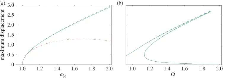
Figure 2.Duffing oscillator example withω=1 andα=0.5: (a) backbone curves and (b) forced response curves when
ζ =0.01 andR=0.1. The solid line shows the exact computation using AUTO; the dashed line shows the result of the
second-order normal form calculation; and the dashed-dotted line the result of the first-order normal form.
Applying the normal form transformation in a similar way to the second-order matrix formulation, now usingu=[uu¯]Tgives
x=U1
1− 3αU
2 1
16ω2n1
cos(ωr1t)+ α
32ω2n1U
3
1cos(3ωr1t), with:ωr1=ωn1+ 3α
8ωn1U 2
1 (3.22)
[7,12]. Note that hereU1 does not fully represent the amplitude of the resonant response. This
is because, when identifying the transform, only the eiωr1t terms are kept in the first equation of
motion inUwith e−iωr1t terms being represented in the transform and vice versa for the second
equation of motion [8].
The response (or backbone) curves for both the second- and the first-order variants of the normal forms, (3.21) and (3.22), respectively, are shown in figure 2a. For comparison, the solution derived using numerical continuation, using AUTO [26], in which no assumptions are made regarding the smallness of terms, is also shown. It can be seen that at low amplitudes, corresponding to weaker nonlinear terms, there is good agreement in the prediction of the response frequency, however as the amplitude increases the higher power terms become significant, firstly for the first-order normal form approximation at about 0.6 and then also for the second-order version at about 1.8.Figure 2bcompares the second-order normal form and the AUTO predictions of a forced response, again it can be seen that good agreement is achieved.
4. Application to nonlinear normal modes
We now consider how the application of normal forms to unforced, undamped second-order differential equations can be used to calculate the NNMs of a system. Second-order normal forms can be used to derive the backbone curves of a system via the resonant responses (e.g. Wagg & Neild [24] or Hill et al. [27]). Here, we extend this to finding the NNM mode shapes, which requires both the resonant response and also the harmonics captured inh. While the technique is general, to facilitate the discussion we apply it to a well-known nonlinear system—the dynamics of a taut cable. Specifically, we will consider the interactions between the first out-of- and in-plane modes (we use mode to indicate the modes of the linearized system). In doing this, to calculate the associated NNMs, we will derive the harmonics excited inallmodes due to resonant responses in the first out-of- and in-plane modes.
14
rsta.r
oy
alsociet
ypublishing
.or
g
Phil.T
ran
s.R
.So
c.A
37
3
:2
0140404
...gravitational sag and tension effects. The motion of the cable out-of- and in-plane (where in-plane relates to the plane in which gravitational sag occurs) are represented as
v(x,t)=
n
φn(x)yn(t) and w(x,t)=ws(x)+
n
ψn(x)zn(t), (4.1)
wherexis the distance from one of the supports and the other support is positioned atx=. Here,
φn(x) andψn(x) are thenth out-of- and in-plane linear mode shapes, respectively,yn(t) andzn(t)
represent the modal contributions for thenth modes andws(x) captures the static sag in the cable
(noting thatvandware defined as zero on the chord line between the supports). The dynamics for thenth out-of- and in-plane modes may be expressed as
¨
yn+ω2ynyn+
k
νnk
m yn(y
2
k+z2k)+
k
2βnk
m ynzk=0
and z¨n+ω2znzn+
k
νnk
m zn(y
2
k+z2k)+
k
2βnk
m znzk+
k
βkn
m (y
2
k+z2k)=0, ⎫ ⎪ ⎪ ⎪ ⎪ ⎪ ⎬ ⎪ ⎪ ⎪ ⎪ ⎪ ⎭ (4.2)
respectively. Here, modal damping and external forcing terms have been removed from the original derivation in line with investigating the backbone curves of the system. Parametersm,
βijandνijare given in Warnitchaiet al.[28] and Gonzalez-Buelgaet al.[29], but importantlyβijis
zero for evenj. The natural frequencies of the out-of-plane modes are proportional to the mode numbern, and for evenn, natural frequencies for the in-plane modes match those of the out-of-plane ones. For oddn, the in-plane natural frequencies are slightly higher than the out-of-plane ones, again see [28,29]. The in-plane axis is defined as positive down, and so gravitational sag is positive.
Gonzalez-Buelgaet al.[29] considered these equations in terms of internal resonance showing that 1 : 1 resonance occurs between the second out-of- and in-plane modes and Macdonaldet al.
[30] generalized this for thenth out-of- and in-plane modes. In addition, they both show that 2 : 1 resonance can occur, but only for the case where the cable is inclined. Hillet al.[27] identified the backbone curves when the system is reduced to the first out-of- and in-plane modes. Here, we build on this work by deriving algebraic expressions for the NNMs associated with these backbone curves, which requires not only the resonant responses of the two modes but also the harmonic response in all modes. To do this, we first calculate the backbone curves along with expressions that capture the harmonics contained in the response. These are then used to find the NNMs in terms of just the two first modes and finally the additional modal contribution due to harmonics in other modes is added to give the full NNM expressions.
(a) Resonant equation of motion and harmonic response
Letting q=(y1 z1)T the modal equation of motion for the reduced two-mode model may be
written in the formq¨+Λq+Nq(q)=0, an unforced version of the left-hand expression in (3.1),
where q= q1 q2
, Λ=
ccω2
y1 0
0 ω2z1
and N(1)q = ⎛ ⎜ ⎜ ⎝ c ν 11
m (q
3
1+q1q22)+2
β11
m
(q1q2)
ν
11
m (q
3
2+q21q2)+
β11
m
(q21+3q22)
⎞ ⎟ ⎟ ⎠.
Here, takingNq(q)=kNq(k)(q), all the nonlinear terms have been placed inN(1)q . As there is
no forcing,v=qand soN(1)v (v)=N(1)q (q). To calculate the nonlinear transform, see (3.4),N(1)v (u) is considered. Rewriting this nonlinear vector in terms ofu, where, for thekth coordinateuk= uk+ ¯uk, gives
N(1)v (u)=ν11
m
⎛
⎝(u1+ ¯u1)3+(u1+ ¯u1)(u2+ ¯u2)2
(u2+ ¯u2)3+(u1+ ¯u1)2(u2+ ¯u2)
⎞ ⎠+ β11
m
⎛
⎝ 2(u1+ ¯u1)(u2+ ¯u2)
(u1+ ¯u1)2+3(u2+ ¯u2)2
15
rsta.r
oy
alsociet
ypublishing
.or
g
Phil.T
ran
s.R
.So
c.A
37
3
:2
0140404
...
This can now be expressed in matrix formn∗vu∗(u,u¯,r,r¯), see (3.13) along with (3.6), and the matrix
β∗can be derived using (3.15), where it can be assumed that, due to the closeness of the natural frequencies, we can write the response frequencies asωr1=ωr2. Using (3.17), the nonlinear vector
in the transformed equation of motion and the transformation vector can be written as
Nu(1)=ν11
m
⎛
⎝3u1u¯1u1+2u2u¯2u1+u1u¯22+ ¯u1u22
3u2u¯2u2+2u1u¯1u2+u21u¯2+ ¯u21u2
⎞
⎠ (4.3)
and
h(1)= ν11
8mω2r1
⎛
⎝u31+ ¯u31+u1u22+ ¯u1u¯22
u3
2+ ¯u32+u21u2+ ¯u21u¯2
⎞
⎠+ β11
3mω2r1
⎛
⎝ 2(u1u2+ ¯u1u¯2)−6(u1u¯2+ ¯u1u2)
u2
1+ ¯u21+3(u22+ ¯u22)−6u1u¯1−18u2u¯2
⎞ ⎠,
(4.4)
respectively. The modal response of the system can now be written asq=v=u+h(1), whereh(1)
captures the harmonic content of the response.
Using the steady-state solution (3.20), the transformed equations of motion,u¨+Λu+Nu(1)=0,
can be written as
!
ω2
y1−ωr21+
ν11
4m[3U
2
1+(2+p)U22]
"
U1=0 (4.5)
and
!
ω2
z1−ω2r1+
ν11
4m[(2+p)U
2
1+3U22]
"
U2=0, (4.6)
wherep=cos(2(φ1−φ2)) with the condition sin(2(φ1−φ2))=0 to ensure (4.3) is real. This allows
possible solutionsp= ±1. It can be shown that onlyp= −1 gives physically meaningful solutions (asωz1=ωy1) which means that when both linear modes are present, they are±90◦out-of-phase,
see Hillet al.[27] for a more detailed discussion of this.
(b) Backbone curves and modal response
Taking the physically meaningfulp= −1 case, there are two semi-trivial solutions for (4.5) and (4.6) in which only one of the two linear modes is resonant
S1 : ωr21=ω2y1+ 3ν11 4m U
2
1, U2=0 (4.7)
and
S2 : ω2r1=ω2z1+ 3ν11 4m U
2
2, U1=0, (4.8)
and two further solutions exist in which both linear modes are resonant
S3±: ω2r1=ωy21+ν11 4m(3U
2
1+U22), U22=U21−
2m ν11(ω
2
z1−ω2y1). (4.9)
Asωz1> ωy1, it can be seen that valid solutions forS3 only exist ifU1≥2m(ω2z1−ω2y1)/ν11. The
point at whichU1=2m(ω2z1−ω2y1)/ν11results inU2=0 and lies on backbone curveS1, see (4.8).
Hence theseS3 solutions (there are two solutions relating to the relative phase of the two linear modes being±90◦, solutionsS3±) are branches fromS1 following a bifurcation atU2=0. This
16
rsta.r
oy
alsociet
ypublishing
.or
g
Phil.T
ran
s.R
.So
c.A
37
3
:2
[image:16.493.64.435.40.286.2]0140404
...
28 30 32
W 34 36 38
0 0.01 0.02 0.03 0.04 0.05 0.06
S1s
S1u S3±
U1
−0.02 0 0.02
−3.5 −3.0 −2.5 −2.0 −1.5
(a) (b)
y1 z1
(×10
−3
)
−0.05 0 0.05
−6 −5 −4 −3
y1 z1
(×10
−3)
−0.04 0 0.04
−0.02 −0.01 0 0.01
y1 z1
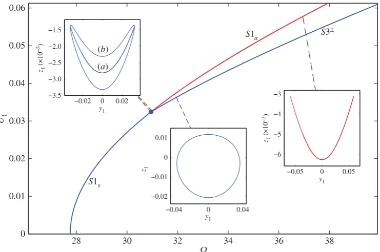
Figure 3.Backbone curvesS1 andS3±for a cable with inset panels showing the motion in projectionq1=y1versusq2=z1.
The inset panel for the response near the bifurcation contains two responses; the response line (a) corresponding to a point on
S1sjust below the bifurcation and the response loop (b) corresponding to a point onS3+just above the bifurcation. Subscripts
sanduindicate that backbone curveS1 is stable below and unstable above the bifurcation.
Using the transform equation,q=v=u+h(1), and the steady-state solution (3.20) gives the response of the modal coordinates
y1=U1cos(ωr1t)+ ν11
32mω2r1U1(U
2
1−U22) cos(3ωr1t)
+ β11
3mω2
r1
U1U2sin(2ωr1t)
and z1=U2sin(ωr1t)+ ν11
32mω2r1U2(U
2
1−U22) sin(3ωr1t)
+ β11
6mω2r1(U
2
1−3U22) cos(2ωr1t)− β11
2mω2r1(U
2
1+3U22),
⎫ ⎪ ⎪ ⎪ ⎪ ⎪ ⎪ ⎪ ⎪ ⎪ ⎪ ⎪ ⎪ ⎪ ⎬ ⎪ ⎪ ⎪ ⎪ ⎪ ⎪ ⎪ ⎪ ⎪ ⎪ ⎪ ⎪ ⎪ ⎭
(4.10)
when the phase difference isφ2−φ1=90◦andφ1has been set to zero.
The S2 solution consists of purely in-plane resonant motion as U1=0. In this case, the
response given by (4.10) reduces to purely in-plane motion. Harmonics exist in this motion including a static displacement which, as it is negative, reduces the apparent sag of the cable during resonance. For theS1 solution, which is resonant purely in the out-of-plane direction as
U2=0, there are also harmonic components in the out-of-plane response. In addition, there is an
amplitude-dependent in-plane non-resonant response. For theS1 solution example of the motion of the mid-span of the cable (where the mode shapes are unity) in they1versusz1plane are shown
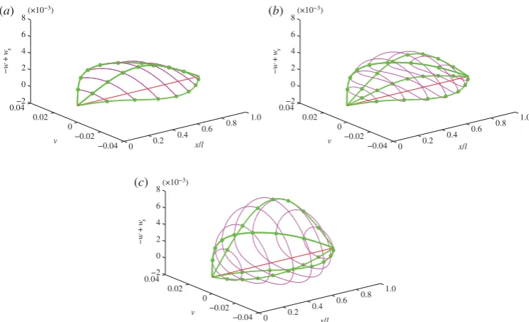
as infigure 3as inset plots. Note that in contrast to Hillet al.[27], these inset panels include the harmonic components as well as the resonant ones. Examples of the more complex motion of the
S3 solution, in which there is 90◦out-of-phase resonant motion in both planes, are also shown in