Abstract Execution in a Multi-Tasking Environment

Abstract Execution in a

Multi-Tasking Environment

The Harvard community has made this

article openly available.

Please share

how

this access benefits you. Your story matters

Citation

Mazières, David and Michael D. Smith. 1994. Abstract Execution in

a Multi-Tasking Environment. Harvard Computer Science Group

Technical Report TR-31-94.

Citable link

http://nrs.harvard.edu/urn-3:HUL.InstRepos:26506448

Terms of Use

This article was downloaded from Harvard University’s DASH

repository, and is made available under the terms and conditions

applicable to Other Posted Material, as set forth at

http://

Abstract Execution in a Multi-Tasking

Environment

David Mazi`eres

Michael D. Smith

TR-31-94

November 1994

Center for Research in Computing Technology

Harvard University

Abstract Execution in a Multi-Tasking Environment

David Mazi`

eres

Michael D. Smith

Abstract

Tracing software execution is an important part of understanding system performance. Raw CPU power has been increasing at a rate far greater than memory and I/O bandwidth, with the result that the performance of client/server and I/O-bound applications is not scaling as one might hope. Unfortunately, the behavior of these types of applications is particularly sensitive to the kinds of distortion induced by traditional tracing methods, so that current traces are either incomplete or of questionable accuracy. Abstract execution is a powerful tracing technique which was invented to speed the tracing of single processes and to store trace data more compactly. In this work, abstract execution was extended to trace multi-tasking workloads. The resulting system is more than 5 times faster than other current methods of gathering multi-tasking traces, and can therefore generate traces with far less time distortion.

1

Introduction

1.1

The Need for Multi-Tasking Address Traces

As computers continue to get faster, the gap between CPU speed and memory and I/O subsystems will continue to widen. Popular benchmarks such as the SPEC benchmark suite have tended to deemphasize the importance of this gap on overall system performance by systematically including only applications that stress raw CPU power over memory and I/O bandwidth. Of all the SPEC benchmarks, the one that seems to be scaling the least well with processor speed isgcc. A recent study of Ultrix performance on an R2000[NUM92] found that thegcc benchmark also spends much more time in system calls than any of the other benchmarks. Furthermore, the SPECgcc benchmark is only the middle phase of the compiler. When the preprocessor and linker are also executed, the problem becomes even worse. Other studies across various platforms have shown that kernel performance is not scaling with processor performance at all[Ous90].

The problem is that many applications do not behave like the SPEC benchmark suite. In particular, CPU-bound programs such as those in SPEC allow the operating system to schedule processes in a way that benefits cache performance. Client/server applications, on the other hand, often have more contexts competing for the CPU and induce frequent context switches by passing messages back and forth. Moreover, many of these applications are sensitive to latency as well as throughput. In a recent study of the X11 Window system, Bradley Chen[Che94] demonstrated the serious impact that this can have on cache performance, particularly when combined with other particularities of the X Window system such as extremely large text segment sizes.

1.2

Existing Approaches to Tracing

Existing execution tracing methods fall into two basic categories: Hardware approaches and software ap-proaches. Hardware tracing involves physically monitoring the pins of a CPU to capture all transactions on the processor-memory bus. Programs are typically modified to emit special markers upon entry to and exit from particular regions of code. This allows tracing hardware to determine specific information about the system activity. For example, one can generate markers upon entry and exit of the kernel idle loop to determine exactly how much time is spent there. The significant advantage of hardware tracing is that it only minimally changes the system’s behavior, and hence can give almost exact timing results. It does, however, severely limit the kind of information one can gather, since all analysis must be performed in real time by the CPU-monitoring hardware. Furthermore, hardware tracing scales poorly to faster and more complex processors, making it extremely difficult to use on newer CPUs.

With software tracing, one executes programs in such a way as to record memory references in main memory, where they can either be directly used in simulation or written out to some form of secondary storage. A special case of software tracing involves modifying microcode to generate trace data automati-cally. More generally, however, programs can be traced through simulation or single-stepped execution, or a program can actually be modified to generate its own trace information as it executes. Software methods unfortunately slow program execution down by at least an order of magnitude, and often several. Such a slowdown can change the order of events and affect the validity of gathered traces. However, with the excep-tion of microcode modificaexcep-tion, software tracing scales well to newer and faster processors. Software traces have already been used for cache analysis[Aga89, BKW90] with great success. By optimizing the tracing process to reduce slowdown, we can obtain traces accurate enough to analyze network-bound applications or simulate radically different processor architectures. The remainder of this section outlines current tracing methods.

1.2.1 Hardware Tracing

A typical hardware tracing tool is Monster[NUM92]—a Tektronix DAS 9200 logic analyzer connected directly to the pins of the MIPS R2000 microprocessor in a DECstation 3100. The Ultrix kernel is modified to emit special markers at the entry and exit of certain regions of code. The state machine in the logic analyzer is then programmed to keep an exact count of events one is interested in studying. The markers are used to restrict analysis to particular regions of code, or simply to record how much time is spent in a given area such as the kernel idle loop. This enables one to track down system performance bottlenecks with great precision.

There are, however, several drawbacks to Monster. It functions well as a counter of events, but generating a full address trace for later simulation is much more difficult. The logic analyzer only contains 512K of RAM, and though it can be triggered to start and stop tracing at specific points of execution, it cannot generate a full address trace over a long period of time. True, one can build logic analyzers with arbitrary amounts of memory, but tens of megabytes of raw data would be generated every second. The act of writing the information to some form of secondary storage would require far longer than actually acquiring the data, and this would leave significant gaps in the trace. Thus, while Monster can give an accurate picture of performance on a DECstation 3100, it is unsuitable for simulating the behavior of systems with different cache or TLB sizes and structures.

It is also difficult and expensive to build a hardware tracing tool like Monster that can sample at the speeds of the newest processors. The R2000 processor analyzed by Monster runs at 16 MHz and has no internal cache. Current processors running at close to ten times that speed will require significantly faster hardware to do the monitoring. Furthermore, as processor speeds continue to increase, CPU to memory buses may not be able to function properly under the additional capacitative loading of a logic analyzer. Already, new high-speed memory systems such as Rambus[Ram] operate in a terminated environment and rely on special packaging to shorten bus lengths and control capacitance.

multi-ported on-chip caches with other accompanying structures such as branch-target buffers become in-tegral parts of processor design philosophies, the problem of monitoring activity between the processor and cache will become almost insurmountable.

1.2.2 Software Tracing

Software approaches to tracing sacrifice the unobtrusiveness of hardware tracing for the ability to scale with processor speed and complexity. The most basic form of software tracing consists of recording all interesting events that occur as one single steps a program through use of the Unix system callptrace.1

This approach is easy to implement and scales well to faster processors, but introducing system call and context switch overhead for every traced instruction executed will slow the traced process down by a thousand times or more. Such a slowdown makes aptrace-based approach unsuitable for tracing anything but the simplest of programs.

An approach similar to ptrace-based methods is that of simulating software execution to obtain trace data. One of the most advanced software simulators isShade[CK]. Shadeallows one to trace only a particular subset of instructions such as all loads and stores. Highly optimized code is constructed at run time to execute blocks of the simulated instructions on the processor in real time. Whenever a traced instruction appears,

Shade invokes a user function to perform whatever analysis is desired by the user. Even with empty user analysis functions, however, a load and store traced simulation of a typical integer benchmark will run 15 times slower than the original program.

In an attempt to combine the benefits of hardware tracing with the flexibility and completeness of software tracing, Agarwal[Aga89] modified the microcode of a VAX 8200 to generate a full address trace of all instructions executed, a scheme he called Address Tracing Using Microcode (ATUM). In ATUM, the modified microcode reserves a portion of main memory on bootup, and makes that region inaccessible to the operating system. TheXFC“microcode extension” instruction can be used to turn tracing on or off, and to read words from reserved memory. Typically, a process enables tracing and sleeps until the buffer fills. When the buffer fills, tracing is automatically shut off and the sleeping process awakens to read back the trace data and write it to secondary storage. Once the buffer has been emptied, tracing is resumed.

ATUM has been used very successfully for detailed cache analysis. It has a significant advantage over other software tracing methods in that tracing the operating system is no more difficult than tracing user processes. ATUM does, however, induce a ten-times slowdown, which is compensated for by slowing the clock interrupt. Another disadvantage of ATUM is the distortion caused by processing the buffer. When the buffer fills up and tracing is turned off, the system continues to run as usual, making exact traces of more than half a million references impossible. To analyze the system over long periods of time, then, one must simulate long traces by stitching together shorter ones. This, in turn, requires compensating for the gaps while analyzing the data. A more fundamental problem with ATUM is the fact that it cannot be implemented on RISC processors with hardwired control.

In order to bring the slowdown of software tracing to a usable level without relying on microcode, then, most software tracing programs actually embed tracing code in the executable image of the program being traced. This process, known as “instrumenting” an executable, can occur at compile-time, link-time, or after link-time. One of the most well-known such software tracing tools is Earl Killian’s toolpixie[Smi91]. Pixie

modifies preexisting MIPS executables to emit all the information necessary to regenerate a full instruction and data address trace. When pixie instruments an executable for instruction and data tracing, it adds instrumentation code at the beginning of every basic block,2

and at each load and store instruction. The markers are eventually written to file descriptor 19 of the process being traced, where they can easily be decoded into an address trace and run through a simulator.

A pixie-instrumented executable will generate a full instruction and data address trace of a program in approximately 15 times the original, untraced execution time of the program. With this tolerable slowdown,

pixie has proved an invaluable tool for analyzing the performance CPU-bound programs such as the SPEC benchmark suite. But pixie is not capable of meaningfully tracing all programs. In particular, certain assumptions about a program being “well-behaved” must be made when rewriting an executable. Often

1

The details ofptraceare described in the manual pages of BSD 4.4, as well as most other Unix operating systems.

2

hand-written assembly code—and occasionally compiler-generated code—will not obey these assumptions.

Pixie, for instance, since it changes the addresses of all functions by adding instrumentation code, is unable to translate the address of a function that is passed to the sigvec system call. As a result, pixie cannot trace programs with signal handlers.

Specific inconveniences such as the inability to handle signals could be fixed up on a case by case basis. There are, however, some fundamental limitations to tracing with a tool like pixie, which become more immediate concerns if one attempts to use the same approach to trace a multi-tasking workload. Though the speedup of pixie over ptrace-based methods makes it possible to gather useful traces in a reasonable amount of time, the remaining slowdown is enough to make most asynchronous events appear to occur instantaneously. This, combined with any extra page-faults incurred as a result of a text segment dilated with instrumentation code, can affect the behavior of the scheduler and distort multi-tasking results.

Nonetheless, pixie-like tools have successfully been expanded to generate exact traces of multi-tasking workloads. Borg, Kessler, and Wall[BKW90] developed such a tool to trace Titan workloads at the DEC WRL. Their system uses link-time instrumentation to insert branches to tracing code at every load, store, and basic block entrance. This enables them to capture all loads, stores, and instruction fetches, but does not record the location of loads and stores within their basic blocks. For efficiency, they reserve 5 of the 64 general-purpose registers in the Titan for use by instrumentation code. All trace information is written to a global buffer which is mapped into the top of every process’s virtual address space. At each entry to or exit from the kernel, a marker containing the current process id and whether the switch is into or out of the kernel is written to the buffer. When the buffer overflows, all traced processes block and a special high-priority process is scheduled to compress and store the buffer contents, or to use it immediately in simulation.

The execution time of instrumented executables in the Titan tracing system is 8–12 times longer than nor-mal. To compensate for this time-dilation and to increase the applicability of the simulations to faster, newer RISC processors, the process switch time is increased by a factor of 16. Unfortunately, cache simulations tend to consume data 10 times more slowly than this system can create it. Therefore, with a 32 megabyte buffer filling up approximately every second, this system is forced to suspend execution of programs for long periods of time. Despite this slowdown, the Titan work was able to make excellent predictions about the behavior of very large caches with various degrees of associativity. The ideas developed during the Titan project form the basis of the approach described in this document.

Bradley Chen[Che93, Che94] at CMU later extended the Titan tracing method to trace the MIPS proces-sor using a modified version of the tracing toolepoxie[Wal92]. Epoxie modifies executables prior to linking them, so as to reduce the size of the rewritten executable. One typically combines all object modules into one big object module, using the commandld -r, runsepoxieon the resulting object file, and finally turns the output of epoxieinto ana.outformat file by invokinglda second time. Thus, while tracing tools that rewritea.outexecutables need to translate register jumps at runtime from large translation tables,epoxie

manages to have the linker perform translations, and therefore produces much smaller executables.

Unfortunately, the MIPS architecture contains only 32 registers: One is hardwired to zero, two are reserved by the kernel for fast TLB miss handling, and the other 29 may all be used by the compiler.3

Thus, where the Titan tracing system could simply reserve five registers for use by the instrumentation code,

epoxiemust actually perform “register stealing,” which means saving and restoring “shadow registers” from memory wherever the stolen registers are used in the original object file. This vastly complicates mapping a single global buffer into every address space, as the current location cannot be shared between processes in a register. As a result, each traced process maintains its own buffer in Chen’s system. At every entry into the kernel, the contents of the current process’s trace buffer is copied by the kernel into a system trace buffer, and the trace is consumed or stored whenever the system trace buffer overflows.

Chen’s system is also able to trace both the Ultrix and Mach kernels. In each case, slightly under 1,000 lines oflocore.swere instrumented by hand, while the rest of the kernel was instrumented automatically by the modifiedepoxie. Since instrumented executables run approximately 15 times slower, the clock is also slowed down by a factor of 15. TLB misses do occur more frequently because of larger text segments, but instead of relying on traces of the user4_{TLB miss handler to study TLB misses, the TLB can be simulated}

3

In reality, one MIPS register,$1, is reserved for the assembler to expand compiler-generated pseudo-instructions.

4_{Most of the kernel resides in unmapped memory for MIPS operating systems. Hence the kernel does not cause many TLB}

from the user instruction address traces which correspond to locations in the uninstrumented executable. Of course, I/O requests still appear to complete 15 times more quickly than they would during untraced execution. Tracing therefore affects scheduler policy despite slowing down the system clock. Scheduler policy, in turn, affects the performance of CPU-bound workloads, where processes scheduled for longer periods of time experience better cache performance because of temporal locality. These CPU-bound processes, however, are precisely those which can already be analyzed with a tool such as pixie. Chen therefore concentrated on analysis of applications where client/server behavior dictates process scheduling.

1.3

Our Approach

The passivity of hardware tracing approaches is quite desirable. Unfortunately, as we have seen, hardware tracing is not general enough to simulate arbitrary architectures, and will no longer be feasible on newer processors. Software tracing, on the other hand, though more difficult, has already proven to be both possible and useful. The most serious difficulty it presents is time dilation. Not only will a 10–15 times slowdown affect process scheduling, it will give I/O the appearance of being an order of magnitude faster than it actually is.

Now that software tracing of multi-tasking and system workloads has been shown to be possible, we must increase its usefulness by finding ways of minimizing the drawbacks, time-dilation in particular. This will allow us to gather useful traces of I/O-bound workloads, in particular network applications. The work presented here shows how tracing overhead can be reduced more than five times through the use of a technique called Abstract Execution[Lar90], in which much of the overhead of producing a full address trace can be postponed to analysis time. The system described in this paper is based on the toolqpt, which uses Abstract Execution to generate very efficient address traces of a single process.

Qpt was modified to work in a multi-tasking environment, and support for the tracing was added to the 4.4 BSD kernel. Extending qptto trace multiple processes had no negative impact on performance. In fact, certain optimizations were added to qpt that would not have been possible without kernel support. For example, costly bounds checking on the buffer is now performed automatically by the VM system. The current implementation only traces user level processes; however, it has been designed with the objective of eventually being able to trace the kernel.

Section 2 describes abstract execution, a powerful optimization to traditional methods of tracing a single process. Section 3 explains how we extended abstract execution to trace multiple processes. Section 4 describes the results of our approach, concentrating specifically on performance of the first implementation. Section 5 discusses further optimizations that can be made to the current system, and how it can be extended to trace the kernel. Finally, we end with a brief conclusion in section 6.

2

Abstract Execution

2.1

Motivation for Abstract Execution

Ptrace-based tracing methods suffer from too much information being made available about the traced process: For each instruction traced, the program under study is completely frozen, and its entire state is made available to the parent process, which must look at the instruction, decide if the instruction is interesting, and if so what registers in the child process also need to be looked at. With pixie, on the other hand, the program is modified to do its own tracing, and output only the information considered interesting—an address trace in our case.5 _{In order to do this,}

pixie must add code for every load, store, and basic block entry. Turning a traced program’spixie output into an address trace is completely trivial, but program execution is slowed down significantly to produce such full output.

The best solution for tracing, then, is to take the advantage of pixie one step further—to record far less than a full address trace at execution time. The program under study should only emit markers for a minimal subset of interesting events at run time. The rest can be deduced at a later point as one analyzes the trace data. That way time dilation on an instrumented executable can be minimized, but a full address trace can still be generated without nearly the overhead of simulating the program under study. The idea

5_Pixie

}

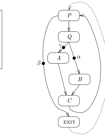
while (P) { if (Q)

A; else

B; C;

C

exit

α β

γ

P

Q

A

B

Figure 1: Simple procedure and corresponding CFG.

of instrumenting an executable but deferring parts of trace generation to a later time is the key to Abstract Execution[Lar90]. Section 2.2 explains which subsets of events it is sufficient to record at runtime, and gives a method for choosing such a subset with a low execution cost. Section 2.3 describes the specifics of implementing abstract execution on the SPARC.

2.2

Overview of Abstract Execution

Let us first consider the problem of minimizing tracing overhead while gathering a full

B

exit

P

A

Figure 2: Edge and block trace. instruction trace of a single procedure; later we will see that tracing multiple procedures

and generating data traces are extensions to the same basic approach. Figure 1 shows a very simple procedure and its associated control flow graph: Each node in the graph corresponds to a basic block of the program, and each directed edge to a possible transfer of control flow. Let us call the set of vertices in this graphV and the set of edgesE. We wish to insert instrumentation along edges and in basic blocks of the program so that every possible execution path fromPtoexitleaves a different trace. In addition, we would like

to minimize the number of times that instrumentation code needs to be executed during a typical execution of the procedure. Given a mixed set of edges and vertices which have been instrumented, one can, for each instrumented vertex, instrument instead the set of all its outgoing edges. Since, by the definition of basic block, a vertex is traversed exactly as many times as the sum of all its outgoing edges, the exchange cannot increase the number of times instrumentation code is invoked in any execution of the program. Figure 2, however, is an example showing that instrumenting vertices can be more expensive than

instrumenting edges. If, for instance, one must instrument only vertices, instrumentation code will have to be added toAandB. Execution pathP →A→B →exitwill execute two pieces of instrumentation code.

If, on the other hand, the two dotted edges are instrumented, only one piece of instrumentation code needs to be executed per invocation of the procedure. For this reason, we always choose to instrument edges rather than vertices.

2.2.1 Terminology

• Any vertex with two or more outgoing edges is known as a predicate. In Figure 1, P andQ are both

predicates.

• A marker emitted by an instrumented edge is known as a witness. If, for instance, the black dots on edges represent instrumentation code in Figure 1, we say that edgeQ→Awrites witnessγ.

• We say there exists a witness-free path between two vertices a and b of a CFG if there exists a set of zero or more vertices xi such that there exist edges a→x1 → x2 → · · · →b which do not write

witnesses. If we represent instrumented edges with dots as in Figure 1, this means that there exists a directed path fromatobwhich does not cross any black dots.

• Given a CFG, thewitness set of a predicatepwith respect to an edgep→q, writtenwitness(p, q), is defined as follows:

Ifp→qwrites witnessτ, thenwitness(p, q) ={τ}.

Ifp→qdoes not write a witness, thenwitness(p, q) contains any witnessυsuch that there exists a witness-freepath fromq to some vertexx, and an edgex→y which writesυ.

In addition, ifp→qdoes not write a witness and there exists awitness-freepath fromqtoexit,

witness(p, q) also contains the special witnesseof.

Put more simply, a witness is inwitness(p, q) if it can be the next witness recorded when edgep→q

is executed. In the case of the example CFG,witness(P, Q) ={α, γ}.

2.2.2 Solving the Tracing Problem

The problem of being able to regenerate an instruction address trace from a set of witnesses is equivalent to determining exactly which outgoing edge was executed from each predicate. Given a predicate p and outgoing edgesp→q1, p→q2, . . . , p→qn, we will be able to determine which outgoing edge was taken

from the next witness if and only ifwitness(p, qi)∩witness(p, qj) =∅ when i6=j. In other words, if some

witness τ can potentially be the first witness recorded when either of two distinct edgesp→qi andp→qj

is traversed, then there will be no way of disambiguating the two edges whenτis read back from the witness file after executing the instrumented program.

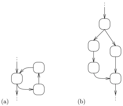
If a CFG has the set of vertices V and the set of edges E, then a set of edgesepl ⊆E solves thetracing problem when one can instrument only the edges inepl and still have disjunctwitness-setsfor the outgoing edges of every predicate inV. There are two cases which clearly do not satisfy thetracing problem, illustrated in Figure 3 on the next page: IfE −epl contains a directed cycle, in other words there is a witness-free path containing a program loop, there will be no way of knowing how many times the loop is executed. In our example of Figure 1 on the preceding page, suppose that edgeQ→B were not instrumented. The path

P → Q→ B → C → P is now witness-free. Thus β is now inwitness(P, Q) as well as witness(P,exit).

If at vertex P we read β from the witness file, we will have no way of knowing if the next vertex isQ or

exit. Another case which does not satisfy thetracing problem is when E−epl contains a diamond. A set

of edges contains a diamond if it contains loop-free pathsp→a→ · · · →xand p→b→ · · · →xwhich are disjoint except forpand x. It is clear thatwitness(p, a)∩witness(p, b) will contain the first witness of any path between xandexit. (If no such witnesses exists, then both witness-sets will containeof.)

Conversely, if a subset of edges epl does not solve the tracing problem, then E−epl must contain a diamond or loop. To see this, suppose that α∈ witness(p, a)∩witness(p, b) where a 6= b, and that α is generated by edge x→ y. There must exist two witness-free paths from p to x, one of which starts with edge p→a, and the other withp→b. Let z be the first vertex these two paths have in common (z may be the same as x). There are two witness-free paths p→ a→ · · · → xand p →b → · · · → xwhich are disjoint. Either one of them contains a loop, or the pair of them forms a diamond. Therefore, the sets of edges which solve the tracing problem are precisely those whose complements do not contain directed cycles or diamonds.

(b) (a)

Figure 3: Impossiblewitness-free paths: (a) Loop. (b) Diamond.

arrow in Figure 1 on page 6), then the execution counts of the edges in a procedure form a weighting (call it WEX) of the procedure’s CFG, provided that the imaginary edge is assigned the number of times the

procedure has executed. The problem of executing instrumentation code the least number of times, then, is the problem of finding the set of edgeseplwhich solves the tracing problem with the lowest possible sum of weights inWEX.

Of course,WEX is generally not known before the program has been traced or profiled, and will generally

change from execution to execution if the input events of the program are not identical. However, some sets of edges are always better than others. For example, in Figure 1, the weight ofP →Qis equal to the sum of the weights of Q→ Aand Q→B. Thus, it is always better to instrument Q→A andQ→B rather than, say,P →Qand Q→A, even though one can solve the tracing problem with either pair. Thus, one can benefit from finding a solution to the tracing problem which minimizes the weights of the instrumented edges with respect to some weighting, even if that weighting is not the actual execution weighting. One way to obtain such a weighting is to profile or trace the program once with some non-optimal edge placement, and to use the results in instrumenting the executable a second time. As we will see, however, when multiple procedures are traced, there are further restrictions on the placement of instrumentation code which make a two-step instrumentation process not worthwhile. The programqpt used for this multi-tasking tracing work simply calculates a weighting on the assumption that all loops iterate 10 times, and thatifconditionals are true half of the time.

Minimizing the total weight of epl is the same as maximizing E −epl. Unfortunately, finding the maximally-weighted set of edges that does not contain a directed cycle or diamond in any given CFG is not always an easy problem. A slightly more restrictive requirement is thatE−epl contain no directed or undirected cycles whatsoever. A set of edges that reach every vertex of a graph without cycles is simply a spanning tree. A maximum spanning of a CFG can easily be found using Kruskal’s algorithm:6 _{One starts}

with an initially empty set of edges and keeps adding the heaviest edge that does not form a loop until finally one can add no more edges without creating a loop. Larus and Ball[BL91] have shown that for a large class of CFGs, choosing a maximum spanning tree forE−epldoes in fact produce optimal results. For the other types of CFG that exist, they argue that the spanning tree approach is still near-optimal. This approach is therefore used to determineepl in their implementations of Abstract Execution.

There is still one slight qualification that needs to be made to the above method. The edge fromexitto

the first block of the procedure is imaginary, and therefore cannot be instrumented. If the spanning tree does not contain this edge, however, there will be paths through the procedure which do not write any witnesses to the trace file. Consider, for instance, what would occur in Figure 1 if β were to lie on the dotted arrow rather than on edgeP →exit: We would have no way of knowing how many times basic blockP executed,

6_{A more detailed description of Kruskal’s algorithm and a proof of its optimality may be found in [LD91]. The explanation}

because we would not know how many times the procedure executed. We must therefore begin Kruskal’s algorithm with the imaginary edge already in the spanning tree.

2.2.3 Tracing multiple procedures

First, let us consider the case of a program in which control transfers between procedures only through ordinary call instructions. Suppose that vertex Qof Figure 1 contains a call to another procedure—let us call such a vertex a call vertex. The called procedure will also write witnesses to the trace file, including possibly a witness with the same value as β. When regenerating the basic block trace, then, if we see the witness β at vertex P, we will not know whether to follow the edge toexitor proceed toQ and interpret

β as the first witness of the called procedure.

One could possibly avoid this problem by assigning all procedures different witness numbers, though this would severely impact both trace size (since 8-bit witnesses would no longer be usable for small functions), and trace compressibility. However, suppose the procedure called byQcalls its parent procedure in the first basic block, and that this time edgeP →exitis taken—This possibility still prevents us from regenerating a

trace. Thus, to make such a scheme work, all procedures would have to emit a witness upon entry to prevent the possibility of mutual recursion from introducing ambiguities. Furthermore, the added complexity of writing data trace information to the same buffer will make a unique witness number approach even less practical.

To reconstruct a multi-procedure trace, then, we must always know which procedure wrote a byte at the point where we read that byte from the trace file. Ambiguity will arise whenever there exists a witness-free path from a predicate to a call vertex. We must therefore add a witness along each path from a predicate to a call vertex, to block the regeneration program from seeing the child procedure’s witnesses when it might also see a witness from the current procedure. Such a witness is called ablocking witness.

However, if blocking witnesses are not added carefully, more edges may end up being instrumented than necessary. In our example, when we add a blocking witness to edge P → Q, call it δ, we no longer need witnesses on both Q → A and Q → B. If, for instance, we eliminate witness γ along Q → A,

witness(Q, B) ={α}andwitness(Q, A) ={β, δ}, so that the resulting set of instrumented edges still solves the tracing problem. In general, therefore, it is better to place blocking witnesses before calculating the maximum weight spanning tree, as this will prevent redundant witnesses.

A second source of redundant witnesses can occur with multiple call vertices along a predicate-free path. Suppose, for instance, that verticesAandC of Figure 1 are call vertices. If one inserted a blocking witness forC along edge A→C before handlingA, then one would still need to instrument edgeQ→Ato block the procedure call in Afrom predicate Q. If on the other hand, Q→A had been instrumented first, then there would be no need to instrument A →C. Thus, as one proceeds through the list of call vertices to insert appropriate blocking witnesses, they should always be inserted on the outgoing edge of a predicate. Stated formally, for each call vertex aand predicatep, if there is exists a set of zero or more nodesxiwhich

are not predicates and a pathp→x1 →x2→ · · · →a, we must insert a blocking witness on edgep→x1,

orp→ain the case of noxi’s.

Many programs, however, do not jump from one procedure to another exclusively through call instruc-tions. The C functionlongjmp, for instance, loads an address from ajmp bufinto a register and performs an indirect jump to the register. The solution is to record the addresses of the jmp bufs when they are written insetjmpand jumped to inlongjmp. The regeneration program can then map each of the traced program’s jmp bufs to one of its own, and execute a setjmp or longjmpwherever the traced process did. Instrumenting code to record the argument of one of these functions is essentially the same problem as recording the address values of loads or stores. The same algorithm can be used for both, and is described in the next section.

2.2.4 Gathering Data Traces under Abstract Execution

Once we have a way of generating an exact instruction address trace, it becomes much easier to deduce the full set of memory data references. Any procedure with loads and stores will have a particular set of registers which determine the addresses of those loads and stores.7

An instruction which does not modify a register

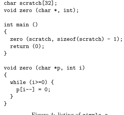
char scratch[32];

void zero (char *, int);

int main () {

zero (scratch, sizeof(scratch) - 1); return (0);

}

void zero (char *p, int i) {

while (i>=0) { p[i--] = 0; }

}

Figure 4: listing ofsimple.c

in that set is considered an easy instruction—it plays no role in the data trace and so can be ignored. An instruction which modifies an important register in a predictable way, such as an increment of a pointer, is considered a difficult instruction. When difficult instructions are encountered, however, no additional instrumentation code is required. Instead, the difficult instruction can be executed by the regeneration program. Impossible instructions are loads of an important register from memory, or return values from functions. Only impossible instructions require extra instrumentation code.

Let I be a memory instruction in procedureP, andR be the set of registers which determine the data address ofI. (For a typical RISC architecture,Rwould only contain one register.) Now letD(I) be the set of all instructions which define one of the registers in R—in other words, the set of all instructions which might last write a register ofR before execution ofI. Now letD∗_{(I) be defined recursively as the set of all}

instructions J inP such that either J ∈ D(I), or there exists an ALU (in other words difficult, rather than impossible) instructionKsuch thatK∈ D∗_{(I) andJ ∈ D}∗_{(K). D}∗_{(I) is called aprogram slicewith respect}

toI.

In order to generate a data trace, then, we must compute the program slice with respect to each load and store instruction. The impossible (non-ALU) instructions in the slice must be instrumented. The hard instructions must be emulated at regeneration time, and instrumentation code must be added at the beginning of the procedure to record any source registers of hard instructions which are live on entry. While calculating program slices, it is trivial additionally to flag as live on entry the argument register of a procedure namedsetjmporlongjmp, if that is required as described in the previous section.

2.3

Qpt

on the SPARC

2.3.1 Background

James Larus[Lar90], who coined the term abstract execution, based two tracing tools on the technique: AE, andqpt. AE, the earlier of the two, was a modification to the GNU C compiler gccthat instrumented code at compile time. As a side affect of compiling,AE also generated a “program schema,” which described the structure of the program being compiled. A second program namedaecwould then compile the schema into C code capable of turning the trace data emitted by the compiled program into a full address trace. Qpt, his second generation tool, has been improved to modify executables directly. Given an executable file a.out,

qpt generates an instrumented executable a.out.qpt and one or more C files containing code capable of turning the output ofa.out.qptinto a full address trace.

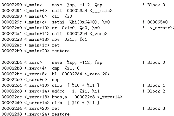
Let us look at a simple example and see how, on the SPARC, we can trace the programsimple.clisted in Figure 4. The result of compiling this program withgcc -Ois given in Figure 5 on the next page.8 _Before

8_Gcc

00002290 <_main> save %sp, -112, %sp ! Block 0 00002294 <_main+4> call 000023a4 <___main>

00002298 <_main+8> clr %i0

0000229c <_main+c> sethi %hi(0x6400), %o0 ! 000065e0 000022a0 <_main+10> or 0x1e0, %o0, %o0 ! <_scratch> 000022a4 <_main+14> call 000022b4 <_zero>

000022a8 <_main+18> mov 0x1f, %o1 000022ac <_main+1c> ret

000022b0 <_main+20> restore

000022b4 <_zero> save %sp, -112, %sp ! Block 0 000022b8 <_zero+4> cmp %i1, 0

000022bc <_zero+8> bl 000022d4 <_zero+20> 000022c0 <_zero+c> nop

000022c4 <_zero+10> clrb [ %i0 + %i1 ] ! Block 1 000022c8 <_zero+14> addcc -1, %i1, %i1 ! Block 2 000022cc <_zero+18> bpos,a 000022c8 <_zero+14>

000022d0 <_zero+1c> clrb [ %i0 + %i1 ]

000022d4 <_zero+20> ret ! Block 3 000022d8 <_zero+24> restore

Figure 5: simple.ccompiled withgcc -O. The “!” character begins comments.

proceeding, however, a few things must be noted about the peculiarities of the SPARC architecture and assembly language. First, unlike other platforms, the destination specifier is always last in SPARC assembly language. Second, only the first 8 registers (named %g0. . .%g7) are global to all functions. However, %g0

is hardwired to zero, and %g5. . .%g7 are reserved for future use and never touched by compiler-generated code[SPA, Appendix D]—which means instrumentation code can always make use of them. The remaining 24 registers, named%i0. . .%i7,%l0. . .%l7, and%o0. . .%o7take part in the register window scheme.

Each function starts off with asaveinstruction. This rotates the register windows, making register %ox

into register %ix, and generating a new set of%land %oregisters.9

Thesave instruction also acts like an add instruction, with its source in the old register window and its destination in the new one. Since the stack pointer is%o6, this allows a new call frame to be allocated at the same time as the register windows are being rotated, and allows the stack pointer to be restored automatically when a function executes arestore

instruction before returning. The first six arguments to functions are passed in the%oregisters (which then become %iregisters in the called function), and the return address is stored in%o7.

There is one other odd instruction to note in Figure 5, and that is the call to function mainthat has been inserted by gcc yet does not appear in the C source code. This function invokes constructors of any global C++ objects when one has linked with C++ modules. In the case of C programs, however, main

returns immediately and the call to it can be ignored.

2.3.2 Instruction and Data Tracing

If we runqpt onsimple, we obtain an instrumented executable calledsimple.qpt, and a C program called

simple sma000.ccapable of generating an address trace forsimple. Let us examine the wayqpt instruments this program to generate a full address trace. First, let us determine the instrumentation code we need to add in order to be able to regenerate a full instruction trace. Since start, the function that calls main, has presumably been instrumented correctly according to the method described in the previous section, there is a blocking witness before the call to main. We therefore already know that we are entering main

whenever we enter it. Sincemaincontains no conditional branches (it is one large basic block), we need add no instrumentation code to it to obtain a full instruction address trace.

9

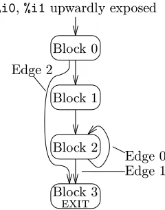
Function zero, on the other hand, contains conditional branches. The control flow graph of zero is depicted in Figure 6, along with the edge and vertex numbers assigned to the function by qpt. Let us find a maximum weight spanning tree of edges not to instrument in function zero. We start by adding the imaginary edge 3 → 0, and make that the first edge in our spanning tree. Next, we must place blocking witnesses between every predicate and call or exit vertex. In this example, this means we are forced to instrument edges 0→3 and 2→3 (which are confusingly numbered 2 and 1 byqpt, respectively). Finally, we must repeatedly add to our spanning tree the most expensive edge that will not cause a loop and that does not already bear a blocking witness. In this example, edge 2→2 (or 0, asqpt numbers it) is the most expensive edge, if we estimate that loops iterate 10 times. However, that edge will form a loop if added to the spanning tree. Therefore, we must add edge 0→1 or 1→2 to the spanning tree. Since these both must have the same weight, either one will be added as the second edge of the tree, and the other will become the third edge. This leaves edges 0→3, 2→3, and 2→2 to be instrumented.

The function zero also contains store instructions in blocks 1

Block 0

%i0,%i1upwardly exposed

Edge 0 Edge 2

Edge 1 Block 2

exit

Block 3 Block 1

Figure 6: CFG for functionzero

and 2 (namely theclrbinstructions—this opcode is an abbreviation for a byte store of register %g0). Let us first compute the slice with respect to the store in block 1. Working backwards from the instruction, we see that no previous instruction in block 1 affects the values of registers%i0or%i1(this is trivial, asclrbis the only instruction in block 1). We then check all predecessor blocks, in this case only block 0. We proceed backwards through block 0 looking for instructions which define%i0or %i1, but before finding any, we land at the first address of the function. We therefore add%i0and

%i1to the list of registers which are used on entry. Next, we must compute the slice with respect to theclrbin block 2. Proceeding backwards, we find anaddccinstruction which defines%i1in terms of itself. We therefore flag this instruction as a difficult instruction, and continue backwards looking for instructions which define %i0

and %i1. As we go through predecessor blocks, we must mark any

blocks we fully explore so as to help performance and avoid any infinite recursion. In this case, we will explore blocks 1 and 0, and then explore block 2 again (since 2 is a predecessor of itself), but proceed no further.

2.3.3 Rewriting an Executable

It is desirable to have the data segment at the same address in instrumented and uninstrumented versions of a program, so as to avoid having to translate all data references when rewriting an executable. However, the data segment of a program immediately follows the text segment in SPARC executables. This prevents us from enlarging the text segment of a program without changing the address of the data segment. To avoid shifting the data segment, then,qpt places the new text segment immediately after the data segment. To preserve the location of the bss segment,10

a qpt-instrumented executable always begins execution by copying the program text to the end of the new bss segment, and zeroing out the location of the old bss segment. Any read-only data in the old text segment also remains in its old location, unmodified by the instrumentation process. The values of addresses that contained program text in the old text segment are replaced by the new addresses of equivalent instructions. This allows for text address translations in Ccase

statements and functions such assigvec.

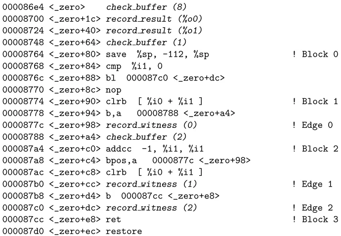
A partial disassembly of simple.qptis shown in Figure 7 on the next page. For readability, instru-mentation code has been replaced by a description of the function. In all cases, however, a pointer to the current location in the buffer is kept in %g6. The value to be recorded is simply moved to register %g7, and stored to the buffer, after which %g6 is incremented by the appropriate amount. Check buffer(n)

checks to see if there are n bytes available in the trace buffer, and branches off to flush the buffer if not.

Record result(r)writes the value of register rto the trace buffer. This takes six instructions because the

10

000086e4 <_zero> check buffer (8)

00008700 <_zero+1c> record result (%o0)

00008724 <_zero+40> record result (%o1)

00008748 <_zero+64> check buffer (1)

00008764 <_zero+80> save %sp, -112, %sp ! Block 0 00008768 <_zero+84> cmp %i1, 0

0000876c <_zero+88> bl 000087c0 <_zero+dc> 00008770 <_zero+8c> nop

00008774 <_zero+90> clrb [ %i0 + %i1 ] ! Block 1 00008778 <_zero+94> b,a 00008788 <_zero+a4>

0000877c <_zero+98> record witness (0) ! Edge 0 00008788 <_zero+a4> check buffer (2)

000087a4 <_zero+c0> addcc -1, %i1, %i1 ! Block 2 000087a8 <_zero+c4> bpos,a 0000877c <_zero+98>

000087ac <_zero+c8> clrb [ %i0 + %i1 ]

000087b0 <_zero+cc> record witness (1) ! Edge 1 000087b8 <_zero+d4> b 000087cc <_zero+e8>

000087c0 <_zero+dc> record witness (2) ! Edge 2 000087cc <_zero+e8> ret ! Block 3 000087d0 <_zero+ec> restore

Figure 7: Disassembly of functionzeroinsimple.qpt

edge markers written to the same buffer are usually only one byte long, but the SPARC architecture does not have unaligned stores. Thus, the register in question is moved to%g7and repeatedly byte-stored to the buffer and right shifted. Record witness(n)simply writes bytento the buffer to record a particular edge having been traversed.

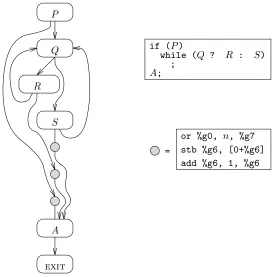
In general, instrumentation code for an edge is always written between the destination block and its predecessor. If the edge from the preceding block, called the “fall-through edge,” is instrumented, then the instrumentation code for that edge is always placed first. This prevents an extra branch to instrumentation code from ever being required on fallthrough edges. All other edge instrumentation code is branched to, however, and all but the last edge must again branch to enter the destination basic block. For this reason, the lastaddinstruction in a basic block is usually moved forward into the delay slot of the outgoing branch. Figure 8 illustrates the typical placement of instrumentation code for a call vertex Awith three predicate predecessors.

Buffer checking will not be covered in detail, for, as we will see in the next section, it is no longer required when performing multi-tasking traces. It suffices to say that the reserved registers in the SPARC architecture are a large advantage for buffer checking, as they allow buffer checks to be placed anywhere with equal cost. On other architectures which use register stealing, one must attempt to place buffer checks only in regions where one has already “stolen” the relevant registers to record a witness or register value. However, a tremendous disadvantage of SPARC is that it is a condition code architecture. In places where condition codes are live across buffer checks, the code to check the buffer without using a comparison or conditional branch is horrendously expensive.

3

Extending

qpt

to a multi-tasking environment

3.1

Design Motivation and Overview

= stb %g6, [0+%g6] add %g6, 1, %g6 or %g0, n, %g7

A;

P

Q

R

S

A

exit

while (Q ? R : S) if (P)

;

Figure 8: Actual placement of instrumentation code for incoming edges to call vertexA.

roughly be broken into two categories: Executing extra instructions required for tracing (and suffering the corresponding cache misses), or managing and consuming the trace data. Abstract execution, as we have seen, addresses both problems by minimizing the number of trace markers which need to be recorded. The challenge, then, was to coordinate shared use of the trace buffer and maintain or enhance the benefits of abstract execution.

Because qpt-instrumented executables often sequentially write the values of several registers directly to the trace buffer, any combination of bytes could potentially be written to the buffer. Using an escape sequence to flag a context switch in the trace buffer is therefore impossible without the use of run-time checks. Though witness numbers are assigned at instrumentation time, and could simply be chosen never to conflict with the chosen escape sequence, register writes would need to be checked against the escape sequence. The actual check could in theory be performed with only two instructions. However, again, as SPARC is a condition-code architecture such checks would be much more expensive with live condition codes. To avoid this problem, the tracing system developed for this work simply records context switch information in a separate buffer, and stores it in a separate file which can then be used to disambiguate the multi-tasking traces.

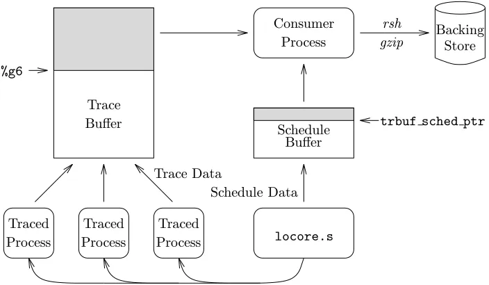
The full tracing procedure chosen for this work, then, is illustrated in Figure 9 on the following page. To avoid the overhead of copying trace data at each context switch, the same global buffer is mapped into all traced processes and the consumer process. These processes all share a single value of register %g6, and use it as a pointer into the trace buffer. locore.s, the interrupt and exception handler, is modified to record context switch information in a special schedule buffer. The schedule buffer is located in kernel memory above the user stack. Its first free location is pointed to by a kernel global variabletrbuf sched ptr. When either the trace buffer or the schedule buffer overflows, the consumer process can store the trace data to a file, or pipe it to another process.

trbuf sched ptr

Process Process

Process

Buffer _Schedule

Buffer

Schedule Data Trace Data

locore.s

Backing

%g6

Store Consumer

Traced Process

Traced Traced

Trace

gzip rsh

Figure 9: Overview of the approach.

best performance results were generally obtained by piping the output ofbdump over the network through thershcommand, and compressing and storing the data on a DEC Alpha workstation with the GNU tool

gzip.

3.2

Implementation Specifics

The following subsections give the implementation specifics of the system, and describe the interface to the kernel portion of the system. Section 3.2.1 explains the setup procedure required for mapping the trace buffer into a traced procedure’s address space, and also the steps required for a consumer process to register itself. Section 3.2.2 discusses the special steps taken during user/kernel and kernel/user transitions which ensure that no ambiguity is introduced with context switches. Finally, Section 3.2.3 describes the method used for detecting buffer overflows and consuming the buffer.

3.2.1 Mapping the Buffers

The Sparcstation VM structure is pictured in Figure 10. The hardware

Dead Zone

Stack

Kernel User Text and Data

f8000000 00004000

20000000

e0000000

Figure 10: Sparcstation VM requires that the most significant three bits of any valid virtual address be

the same, which leaves a 3 Gigabyte gap in the middle of the address space. The lower 512 Megabytes generally contain a program’s text and data, the upper 128 Megabytes are used to map the kernel into every context, and the user stack is located immediately underneath the kernel. The global trace buffer is always mapped into the address space of processes immediately below the 3 Gigabyte dead zone. No reasonable program designed to run on a Sparcstation would attempt to set its break value11

at 512 megabytes. The only danger of a program making specific use of virtual addresses at the location of the buffer is for memory allocated through use of themmap

system call. However, mmapby default starts allocating memory around 32 megabytes, and thus could only fail if the user explicitly requested virtual addresses that conflict with the trace buffer location.12

The trace buffer itself is implemented as a device driver, which is called/dev/trbuf. When the device is first opened, it reserves a portion of non-pageable memory for the global trace buffer. The system currently

11

i.e. the first address beyond the heap, usually only changed bymallocusing thebrkorsbrksystem call.

12

uses a 1 MB buffer, though this size can easily be changed at compile time through modification of a constant

TRBUF SIZE. When the device is first opened, it also initializes a kernel global variabletrbuf g6to contain the value0x20000000−TRBUF SIZE. The buffer can then be mapped into processes with one of two ioctl

system calls—one for traced processes, and one for the consumer process. In order to be able to identify traced processes easily, these calls modify the value of a field calledp trace statwhich has been added to the portion of theprocstructure that is zeroed upon process creation.

When instrumented executables begin execution, they execute the call

ioctl (fd, BIOCMAP)

before jumping to the first instruction of the untraced program. (fd here is the file descriptor number corresponding to the trace buffer.) This maps the trace buffer into the process’s address space. In addition, thep trace statfield is logically OR-ed with the valuePRTRC TRC, to indicate to various parts of the kernel that the process should receive special treatment such as sharing the value of %g6 with all other traced processes. More detail will be provided about the use of this flag in the following two sections. When a consumer process begins execution, it must map the buffer with the call

ioctl (fd, BIOCSMAP, &bufinfo).

(bufinfois simply a structure which gets the start values of the schedule and trace buffers.) This call also maps the trace buffer into the calling process’s virtual address space, but sets the PRTRC ANA flag in its

p trace statfield. This flag also indicates that%g6should be shared with this process, but does not trigger any of the other special behavior required for a traced process.

The Sparcstation MMU performs hardware table walking on TLB misses. However, it only fills the TLB with Page Table Entries from 128 Page Map Entry Groups (or PMEGs) of 64 PTEs each. Since the schedule buffer is written by the kernel inlocore.swith traps disabled, a PMEG miss would put the processor into error mode, and abort execution of the kernel. The schedule buffer is therefore allocated in kernel memory above the stack, where the VM code locks PMEGs and guarantees their continued existence. Though protection on the schedule buffer’s pages could have been changed to allow user-level access, doing so would have required short-circuiting the kernel virtual memory code, and given how small schedule data is in comparison with trace data, this was not worth the effort. Instead, schedule data is simply read from

/dev/trbufusing ordinary file reads.

3.2.2 User/Kernel Transitions

Whenever the kernel is entered from user mode and either PRTRC TRC or PRTRC ANAis set in the current process’s p trace stat field, locore.s has been modified to store the value of %g6 in the kernel global variabletrbuf g6. Before returning to user mode, the return from trap code again checks p trace stat, and if the process requires the shared value of%g6, then that register is restored fromtrbuf g6rather than from the value in the trapframe. Additionally, before returning to user mode, if the schedule buffer is nearly full then the trap code is reentered with a new, fake, trap value calledT SBOF. This causes traced processes to block as if the trace buffer had overflowed. The mechanism employed is identical to the fakeT AST trap which is used to force a reschedule when exiting the kernel. However T SBOF takes precedence overT AST

since it will likely affect the next process to be scheduled.

The first process to open/dev/trbufand perform aBIOCMAP ioctl, then, returns from the system call to find the address of the trace buffer in register %g6. Any subsequent traced process will find that %g6

points to the first free byte of the buffer. Regardless of what other processes have been scheduled since a traced process last ran, that process will always have a pointer to the first free byte of the trace buffer in

%g6. When the trace data is stored by the consumer process, the consumer process can simply point %g6

back to the beginning of the buffer. The problem of disambiguating the concatenated traces is solved by keeping the schedule buffer.

%g6and the PC in the new process’s trapframe. As we will soon see, instrumentation code which causes the buffer to overflow is rolled back, and consequently%g6does not always hold the value0x20000000on buffer overflow. Whenever it rewinds %g6, then, the user-level consumer process is expected to add to its output stream a fake schedule marker with the actual value of%g6at overflow.

Unfortunately, the situation is complicated by the possibility of exceptions or interrupts occurring during the execution of instrumentation code. If a value has been written to the buffer, and a trap or interrupt occurs before the increment of %g6, then information will be lost if a different process is scheduled upon return to user mode. When an interrupt or exception occurs, therefore, the text of the current program must be examined to determine if instrumentation code that makes use of register %g6has just been suspended. If so, since %g6is always incremented last in instrumentation code, the PC is simply rewound to the first instruction of the instrumentation code.

The situation is, of course, complicated still further by the fact that the instructions one wishes to examine are not necessarily in resident pages, or do not necessarily have valid PMEGs currently allocated for them. Since the modified trap handler code must obviously run with traps disabled, one must be very careful in examining the user text segment. In particular, the reason for entering the kernel could actually be a text fault, which may or may not have been caused by instrumentation code spanning two text pages. However, two facts allow us always to recognize instrumentation code at trap time: First, all instrumentation code is straight line code. Witness code does contain a branch, but the branch is delayed, and its target instruction is only executed after the increment of %g6. Second, since we always roll back instrumentation code on a user/kernel transition, the first instruction of an instrumentation code sequence will always be resident if any other instruction in that code sequence is interrupted or causes a trap.

The method employed, then, is to look not at the trap PC, but at the previous instruction. If that instruction is not currently accessible, then the trap instruction is the target of a branch and we can safely assume that the buffer and %g6are in a consistent state. If, on the other hand, the previous instruction is resident and belongs to the middle of an instrumentation code sequence (which we can easily recognize by the fact that it makes use of reserved register %g7 as a temporary register),13 _{then we continue scanning}

backwards, looking for the the first instruction of the sequence, aborting the process at any time if we cross a page boundary and find the page invalid.

3.2.3 Buffer Overflows

Qpt, when tracing single processes, is constantly forced to check for space left in the buffer, and branch off to write the buffer to disk in flush buffer_{whenever there is not enough space left. This can be expensive,} particularly when the checks must occur in places with live condition codes, where the buffer check code cannot make use of conditional branches. In multi-tasking mode, however, traced executables are not responsible for storing their own traces. There is no reason, therefore, to make them responsible for checking free space in the buffer.

Whenever the trace buffer overflows, it causes a memory data fault to occur at address 0x20000000. This is therefore used to detect buffer overflows. Whenever such a fault occurs, and the process causing the fault hasPRTRC TRCset, the memory fault code invokes functiontrbuf blockwith a non-zero argument to block all traced processes, including the currently running one, until the buffer has been processed and reset by the consumer process. When trbuf blockis called, a global kernel variabletrbuf isblockedis set to non-zero, and all runnable traced processes are pulled off the run queue and placed onto a fake sleep queue which is inaccessible to the normal wakeup function. At this point, the process that caused the trap also sleeps, and when it is woken up will return from the memory fault as if a simple PMEG miss had occurred. If, while processes are blocked, any traced processes which were sleeping at trbuf block time are woken up, the wakeup is recorded by logically OR-ingPRTRC WAKwith thep trace statfield of the process’s proc

structure, but the process is not placed back on the run queue until after the consumer process is finished.

13

In reality, the previous instruction may be a branch, preceding the increment of%g6 in a record witness_{sequence. We}

3.3

Comparison

One of the significant disadvantages of Chen’s system over its predecessor was the need to copy trace data multiple times before consuming it. Borg et. al., on the other hand, were able to map the same trace buffer into all processes, which they did by sharing the buffer pointer in a register between all processes. Fortunately, the SPARC ABI by reserving %g5. . .%g7, allowed the system developed for this study to map one buffer globally. It should be noted, however, that though no compiler generated code makes use of these registers, a few of the hand-written assembly-language functions in the BSD libclibrary actually did, and needed to be recoded slightly.

A large disadvantage of both Borg’s and Chen’s systems is the amount of time spent consuming the trace. Consuming trace data in a cache simulation is at best 10 times slower than producing the data. However because of the sheer size of the data in the two previous systems, storing it to disk or tape was even slower. An uncompressed standard address trace requires 5 bytes per trace item. 4 bytes are required to record the address of the memory reference, and one byte is required to record the type (Load, Store, or Basic Block Entry) as well as the length of the reference. In the Titan system, the 32 Megabyte buffer filled up in less than one second of untraced execution. By comparison, abstract execution produces on the order 1–5 megabytes of uncompressed trace data per second of untraced execution. In addition,Qpt’s trace data is quite compressible, and can typically be reduced by another order of magnitude by the GNUgzipcompression utility. Thus, in this system we can execute instrumented programs and store the traces with only slightly higher overhead than the previous systems spend simply executing the instrumented executables.

4

Results

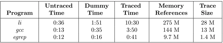
The first round of experiments show that user-level execution time of traced executables, as estimated by the Unix time command, is roughly three to four times greater than that of untraced executables. The global trace buffer fills up at a rate of approximately two-thirds of a byte per memory reference, and can be forwarded across the network, compressed, and stored at a rate of 350 Kbytes per second. As a result, CPU-intensive programs perform the worst under this system, experiencing a slowdown of just under 18 times. This compares very favorably with Borg’s and Chen’s systems, in which the reported slowdown is slightly less, but does not include the time to store or consume the trace—typically an order of magnitude greater than traced execution time in their systems. I/O-bound and interactive programs, on the other hand, did not experience any significant slowdown during execution, and storing the traces only slowed them down by a factor of 3.

In order to characterize performance of the system, two sorts of programs were traced: interactive and non-interactive programs. Performance of interactive programs is difficult to characterize quantitatively, for running time depends on user input, and latency is as important a factor as throughput. Several simple X-windows sample programs were instrumented and traced simultaneously, and their performance was found to be comparable to untraced versions, save for occasional interruptions during buffer processing. This paragraph, for instance, is being typed using an instrumented copy of the simple X-windows text editor

xedit, while an instrumented version of the follow-the-cursor demo program xeyes is also running. During traced execution, the program seems just as fast as normal. For every 40 or so characters that are entered into the buffer, there is an annoying pause for a second or two as the buffer is sent over the network and stored. However, this is not too much worse than auto-saves by theemacstext editor, which may also take a second or two for large buffers saved onto NFS mounted partitions. In short, it is quite reasonable to expect to trace interactive X applications without the user loosing patience and no longer providing a realistic input stream.

Untraced Dummy Traced Memory Trace

Program Time Time Time References Size

li 0:36 1:51 10:30 275 M 28 M

gcc 0:13 0:35 3:50 144 M 13 M

egrep 0:12 0:16 0:41 9.7 M 1.4 M

Figure 11: Traced and Untraced Execution Times

benchmark listed is another subset of the SPECINT92 benchmark suite, and measures the time necessary forgccversion 1.35 to turn one of its own pre-processed source files,1stmt.i, into optimized 68000 assembly code. Finally,egrepis simply theegreputility which came with 4.4 BSD, searching a 5 megabyte input file for a pattern which the file does not contain.

There are three times reported for each program. Untraced time is the execution time of the uninstru-mented program on the chosen input file. Dummy time is the running time of the instruuninstru-mented executable without the time required to store the trace. It was measured by tracing the program as usual, but saving the trace and schedule buffers to /dev/nullrather than to an actual file. Finally, traced time is the time required to run the instrumented executable with a 1 megabyte trace buffer, and pipe the trace information through rsh to a DEC Alpha workstation, where it is compressed with the command gzip --fast and stored to a local disk. Each test was run at least three times, and the numbers reported for all three cases are the most often encountered execution times, which were always also the best times. Occasionally much higher execution times were encountered. For example, the first execution ofgcc took 45 seconds. Most of the extra execution time appeared to take place before the introductory version message was printed out. Since the executables were all on NFS-mounted partitions, this and other delays could be explained by the fact that throughout the experiments a networking project was often flooding the network with packets. For this reason, it seems reasonable to discard high execution times in determining performance for both traced and untraced execution.

As expected, tracing overhead is proportional to the amount of time spent in user-level execution. Both

li andgcc spend over 90% of their execution time in user level, as estimated by thetime command. Li has negligible input and output files, and performs the worst. Gcchas a small amount of I/O, namely a 110 K input file and a 90 K output file. Egrep, on the other hand, spends 90% of the time executing in the kernel or waiting for I/O and performs considerably better. Measuring the performance of CPU-bound benchmarks in the system basically gives us an upper bound on tracing overhead. Programs with lower amounts of user-level CPU utilization execute faster to some extent because by Amdahl’s law a smaller percentage of execution time is affected by the tracing, but another significant part of the improvement is that ratio of the rate of trace data creation to consumption is lower. Fortunately, however, CPU-bound programs are also those whose analysis is least affected by time dilation. Because of their infrequent context switches and ability to scale well with raw integer performance of processors, they are also those least interesting to trace in a multi-tasking context.