The Happiness Trade-Off between Unemployment and Inflation

The happiness tradeoff between

unemployment and inflation

David G. Blanchflower

Department of Economics, Dartmouth College,

Division of Economics, Stirling Management School, University of Stirling, Federal Reserve Bank of Boston,

Peterson Institute for International Economics, IZA, CESifo and NBER

David N.F. Bell

Stirling Management School, University of Stirling, IZA and CPC

Alberto Montagnoli

University of Sheffield

Mirko Moro

Stirling Management School, University of Stirling and ESRI

17th April 2014

Abstract

Unemployment and inflation lower well-being. The macroeconomist Arthur Okun characterized the negative effects of unemployment and inflation by the misery index - the sum of the unemployment and inflation rates. This paper makes use of a large European dataset, covering the period 1975 to 2013, to estimate happiness equations in which an individual subjective measure of life satisfaction is regressed against unemployment and inflation rate (controlling for personal characteristics, country and year fixed effects). We find, conventionally, that both higher unemployment and higher inflation lower well-being. We also discover that unemployment depresses well-being more than inflation. We characterize this well-being trade-off between unemployment and inflation using what we describe as the misery ratio. Our estimates with European data imply that a one percentage point increase in the unemployment rate lowers well-being by more than five times as much as a one percentage point increase in the inflation rate.

.

Keywords

Inflation, Misery index, Unemployment, Well-being, Happiness, Life Satisfaction, Great Recession

1

Unemployment and inflation are major targets of macroeconomic policy because a higher level of either of these variables has an adverse effect on welfare. The macroeconomist, Arthur Okun, developed a measure known as the “misery index” – the sum of the unemployment rate and the inflation rate – which was intended to capture how increased unemployment and inflation reduces national welfare. This measure implicitly assigns equal weights to the inflation and unemployment rates. Thus a period where the unemployment rate is 6 per cent and the inflation rate 3 percent is as bad as one where the unemployment rate is 2 per cent and the inflation rate 7 per cent. There is no empirical justification for the use of equal weights. Indeed, there is no consensus among macroeconomists on the relative size of these weights.

Current macroeconomic policy tends to focus on a central bank whose function is to minimize a quadratic loss function with the economic structure (usually in the form of an IS curve and a Phillips curve) acting as a constraint on feasible combinations of unemployment and inflation. The central bank is required to keep the level of inflation close to target while minimizing the welfare losses associated with unemployment.1 More recently, central banks, including the US Federal Reserve and the Bank of England, introduced explicit labor market targets for monetary policy based on the unemployment rate. However, when the unemployment rate fell more rapidly than expected both central banks broadened the list of measures they would focus on. 2 The critical parameters within this loss function are the weights that the central bank places on unemployment and inflation; their ratio reveals the central bank’s implicit inflation-unemployment tradeoff.

This approach contrasts with directly collecting survey evidence on the public’s assessment of the relative costs of inflation and unemployment (Shiller, 1997). Taking this direct approach a stage further, the rapidly developing study of happiness means that a more evidence-based approach can be taken to investigating the relative welfare costs of unemployment and inflation (Blanchflower and Oswald, 2004, 2011).

1 _{Frequently the loss function is described in terms of the output gap rather than unemployment gap. This requires a}

stable relationship between the deviation of unemployment from its natural rate and the output gap. This relation, known as the Okun’s Law, aims to tell us how much of a country GDP is lost when the unemployment rate is above its natural rate.

2 _{For example in its statement from its March 2014 meeting the FOMC announced that 'To support continued}

progress toward maximum employment and price stability, the Committee today reaffirmed its view that a highly accommodative stance of monetary policy remains appropriate. In determining how long to maintain the current 0 to 1/4 percent target range for the federal funds rate, the Committee will assess progress both realized and expected -toward its objectives of maximum employment and 2 percent inflation. This assessment will take into account a wide range of information, including measures of labor market conditions, indicators of inflation pressures and inflation expectations, and readings on financial developments.

http://www.federalreserve.gov/newsevents/press/monetary/20140319a.htm.

Further details of precisely which labor market variables the FOMC are focusing on was outlined by Governor Janet Yellen in two subsequent speeches 1) in Chicago on March 31st 2104 entitled 'What the Federal Reserve is doing to promote a stronger job market' http://www.federalreserve.gov/newsevents/speech/yellen20140331a.htm and 2) in New York on April 16, 2014 entitled 'Monetary Policy and the Economic Recovery'.

2

In this paper we use individual survey data to determine the relative weights of unemployment and inflation on subjective well-being.3 We use these weights to compute a weighted misery ratio, the tradeoff between inflation and unemployment that is required to maintain subjective well being constant. This approach takes self-reported well-being as a proxy for some underlying concept of utility and treats it as being directly measurable rather than being implicit. Our approach does not assume that utility is implicit in consumers’ revealed preferences. Clearly it shares common ground with Shiller, who focused primarily on the negative welfare effects of inflation. The paper builds on earlier work by DiTella et al (2001, 2003) with a broader list of countries and longer time series that includes the Great Recession. Our paper also utilizes new survey data and a new model specification.

Our survey data comprise observations on more than 1.2 million Europeans over the period, 1975 to 2012 taken from the Eurobarometer Survey which is conducted by the European Commission in all member states one or more times every year.4 Our estimates imply that, across European countries, on average a one percentage point increase in the unemployment rate lowers well-being by over five times as much as a one percentage point increase in the inflation rate. This tradeoff between inflation and unemployment is not constant over time and has been higher during the Great Recession. Furthermore, we find a certain degree of heterogeneity in the inflation-unemployment trade off across European countries as well as socio-demographic groups.

Our estimates suggest that the central bank weights may well differ from the socially preferred weights. The political economy aspects of this finding are interesting, since for many central banks, the elected government sets the inflation target and therefore the implicit tradeoff between inflation and unemployment. The divergence between government and popular views of the appropriate tradeoff raise a number of interesting questions such as the information advantages that the government may enjoy, particularly where the dynamics of inflation and unemployment are taken into account.

Section 1 considers the different approaches that have been developed to deal with welfare losses associated with inflation and unemployment, first by macroeconomists and then by researchers into subjective well-being. Section 2 considers how the misery ratio has changed over time in Europe. Section 3 estimates the size of the marginal rate of substitution between unemployment and inflation along the social welfare function using a dataset which merges Eurobarometer data on individual life satisfaction with macroeconomic data on inflation and unemployment. Is unemployment more costly than inflation? Our answer seems to be 'yes', at least in the period and over the countries considered. Section 4 discusses and interprets these results using a more standard macroeconomic framework. The final section concludes.

1. Welfare Losses Associated with Inflation and Unemployment

3 _{The terms subjective or self-reported well-being, happiness and life satisfaction will be used interchangeably in the}

remainder.

3

Interpretations of the welfare costs of inflation focus on the real resource costs associated with asynchronous price changes or the reallocation of resources to government associated with increases in the money supply (inflation) and the resulting “inflation tax” - see Bailey (1956), Friedman (1971) and Lucas (2000). Models of the costs of inflation associated with asynchronous pricing models include Lucas (1973), Barro (1976), Benabou and Gertner (1993) and Rotemberg and Woodford (1998). For example, using structural VARs, Rotemberg and Woodford assess the relative costs of inflation and unemployment (incomplete stabilization) in a model where prices changes are staggered. The underlying welfare function ultimately depends on consumption and leisure. The welfare losses of inflation are indirect – they are due to the misallocation of resources associated with price instability, rather than due to a direct effect of inflation on utility. Using this analysis to calibrate a welfare loss function based on the price level and the output gap, Woodford (2001) suggests that “the relative weight on the output gap measure should only be about 0.1” (p.47), implicitly concluding that the welfare gains from price stability are significantly greater than those from stabilizing output and therefore unemployment.

Shiller (1997) used public attitudes surveys to investigate directly individual’s perceptions of the costs of inflation. He showed that a primary concern of individuals is that inflation will reduce their standard of living. They also are concerned about being exploited by unscrupulous individuals or companies that cause prices to rise. He summarizes this argument as the “bad-actor-sticky-wage” explanation of the perceived welfare losses from inflation. Shiller’s contribution is quite distinct from other macroeconomic literature on the welfare effects of inflation, which tends to rely on a revealed preference approach to utility.5 Typically, a representative agent’s utility is inferred through observation of her preferences and broader implications for the economy derived by assuming that there are no aggregation issues in moving from the agent to society as a whole.6 This contrasts with efforts to measure utility based on individual surveys. The literature in this field typically assumes that responses to questions relating to “happiness”, “life satisfaction” or “subjective well-being” provide useful information relating to the latent utility measure widely used by economists.7 However, one important distinction to which we subsequently return is that macroeconomists generally take a forward-looking perspective on utility, in that their models frequently seek to maximize current and discounted future utility streams. The motive for asking such questions is to understand how far individuals judge their lives to be satisfactory. Psychologists view it as natural that a concept such as happiness should be studied in part by asking people how they feel. Economists, inured in the revealed-preference tradition, typically find this approach more difficult. Nevertheless, surveys of subjective well-being have attracted the attention of medical statisticians, psychologists, and economists. The latter include Blanchflower and Oswald (2004),

5 _{We treat welfare and utility as synonymous.}

6

Other assumptions regarding the degree of risk aversion and homogeneity between individual and aggregate consumption have to be made, implicitly or explicitly.

7 _{As Krueger (2009) puts it, “I don't think the results are any less significant [for policy makers] if the results are just}

4

Blanchflower (2007), Easterlin (2003), Frey and Stutzer (2002), Gilbert (2006), Graham (2010, 2011), Lucas et al. (2004), Layard (2011), Oswald and Wu (2010); Powdthavee (2010), Smith et al (2005), Ubel et al (2005). In general economists have focused on modelling two fairly simple questions, one on life satisfaction and one on happiness. These are typically asked as follows.

Q1 Happiness – (e.g. from the US General Social Survey)

"Taken all together, how would you say things are these days – would you say that you are very happy, pretty happy or not too happy?"

Q2 Life satisfaction – from the Eurobarometer Surveys

"On the whole, are you very satisfied, fairly satisfied, not very satisfied, or not at all satisfied with the life you lead?"

The standard approach to assessing responses to happiness questions is to estimate an equation with the happiness response as the dependent variable using ordinary least squares (OLS) or ordered logit from a large-scale individual survey. Higher values of the dependent variable are associated with higher levels of happiness. Generally, the use of OLS or ordered logit makes little difference (Ferrer-i-Carbonell and Frijters, 2004). The happiness approach in measuring the effects of inflation and unemployment on welfare is therefore based on estimating regressions of the form (see e.g., Di Tella and MacCulloch, 2006 and Heinz 2007):

(1) Life Satisfactioncti = α Unemploymentct + β Inflationct + γ Being unemployedcti

+ δ Ωcti + γc + ηt + μcti.

5

The size of the signal-to-noise ratio linking utility to subjective measures of well-being cannot be determined, but, from the psychological and medical perspectives, there are corroborating objective measures in relation to subjective well-being. Positive covariance with measures of subjective well-being is observed in assessments of the person’s happiness by friends and family members, assessments of the person’s happiness by his or her spouse, heart rate and blood-pressure measures of response to stress, the risk of coronary heart disease, duration of authentic or so-called Duchenne smiles8, skin-resistance, measures of response to stress, electro-encephalogram measures of prefrontal brain activity and even standing heart rate and blood pressure (Blanchflower et al., 2011).

This approach begs the question as to whether comparisons of life satisfaction across individuals are meaningful given language and cultural differences across countries. This is not an issue in our context as equation (1) estimates within-country effects, holding potential differences constant. 9. Nevertheless, cross-country comparisons are important in that they tell us something about the validity of happiness data. One way to do this is to check for objective measures that might corroborate happiness research’s findings. Blanchflower and Oswald (2008) found that happier nations report systematically lower levels of hypertension. Happiness and blood pressure are negatively correlated across countries (r = -0.6). This seems to represent a first step toward the validation of cross-country estimates. Denmark has the lowest reported levels of high blood pressure in their data. Denmark also has the highest happiness levels. Portugal has the highest reported blood pressure levels and the lowest levels of life satisfaction and happiness. It appears there is a case to take more seriously the subjective happiness measurements made across countries and it seems meaningful to do cross-country comparisons (Blanchflower 2007). Oswald and Wu (2010) using data across states within USA show that there is a match between these subjective measures of well-being and objective measures.

It is apparent that there is a great deal of stability in happiness and life satisfaction equations, no matter what country is looked at, what dataset or time period used, whether the question relates to life satisfaction or happiness, or how the responses are coded (whether in three, four, five or even as many as ten categories). Well-being is correlated with life events such as being unemployed or being married (Clark et al. 2008 and Frijters et al. 2011). In particular, economics research has been focusing on the relationship between income and happiness and interdependence of preferences. In general, Gardner and Oswald (2007) have found that Britons who receive lottery wins of between £1,000 and £120,000 go on to exhibit better psychological health. But individuals in the USA were found to be less happy if their incomes are far above those of the poorest people (Blanchflower and Oswald, 2004). People, however, do appear to compare themselves more with well-off families, so that perhaps they get happier the closer their

8 _{A Duchenne smile occurs when both the zygomatic major and obicularus orus facial muscles fire, and human}

beings identify these as ‘genuine’ smiles (Ekman et al., 1988; Ekman et al., 1990).

9 _{Another way to overcome this is to compare countries where the same language is spoken - Australia, Canada,}

6

income comes to that of rich people around them. Relative income certainly appears to matter. Luttmer (2005), for the USA, finds that higher earnings of neighbors are associated with lower levels of self-reported happiness, controlling for an individual's own income.10 The main findings concerning personal characteristics Ωcti from happiness and life satisfaction equations such as (1) can be summarized as follows.11

Happiness is higher among: Women

Married people The highly educated The healthy

Those with high income

The young and the old – happiness is U-shaped in age

Happiness is lower among:

Newly divorced and separated people Adults in their mid to late 40s

The unemployed The disabled

Immigrants and minorities Those in poor health

Commuters (Kahneman et al, 2004)

Those who live in polluted areas (Levinson, 2012).

Turning our attention to macroeconomic factors, happiness has been found to positively correlate with higher GDP per capita (see e.g., Wolfers and Leigh (2006)). When a nation is poor it appears that extra riches raise happiness. However, income growth in richer countries is not correlated with growth in happiness: this is the Easterlin hypothesis (Easterlin, 1974).12 Alesina et al (2004), find, using a sample of individuals across the USA (1981-1996) and Europe (1975-1992) that individuals have a lower tendency to report themselves as happy when inequality is high, even controlling for individual income. The effect is stronger in Europe than in the USA Di Tella, McCullough and Oswald (2001) show that people are happier when both inflation and unemployment are low. They find that unemployment depresses well-being more than does inflation. This analysis has been updated by Heinz (2010) who found that inflation and unemployment lower life satisfaction in a sample of Western European countries in the period

10

Two facts stand out from studies of life satisfaction and happiness in developed countries. First, it is interesting how little has changed – the distributions in the early 1970s are virtually identical to those observed in 2006. Second, only a very small proportion of respondents report that they were 'not at all satisfied' with their lives, or in the case of the USA, that they were 'not at all happy'. Most people report that they are happy or satisfied with their lives.

11 _{For in-depth reviews on the happiness research in economics see Frey and Stutzer (2002), Di Tella and}

MacCulloch, 2006 and, more recently, Blanchflower and Oswald (2011) and MacKerron, (2012).

12 _{For different points of view regarding the Easterlin paradox see e.g., Wolfers and Stevenson (2008) and Deaton}

7

1990-2002. Wolfers (2003) has shown that greater macro volatility undermines well-being. Wolfers found that eliminating unemployment volatility would raise well-being by an amount roughly equal to that from lowering the average level of unemployment by a quarter of a per cent. Interestingly, the effects of inflation volatility on well-being are markedly smaller. We build on and update these findings below.

2. Misery ratios and views on inflation and unemployment

In this section we introduce an additional measure that captures a different aspect of the interaction of inflation and unemployment from the misery index and more closely aligns with the wellbeing literature - the misery ratio, which is the ratio of the unemployment rate to the inflation rate. Thus, if the unemployment rate is 4% and the inflation rate is 4%, the misery index is 8. But the misery ratio is 1. Below we will link this concept to the marginal rate of substitution between unemployment and inflation – the rate at which at which individuals (or societies) trade off inflation and unemployment, while holding welfare (happiness) constant. The (standard) misery index and misery ratio implicitly assume equal weights for inflation and unemployment rate, while the happiness approach will provide survey evidence on the weights from the subjective well-being perspective. Note that we arbitrarily treat the unemployment rate as the numerator and the inflation rate as the denominator in our misery ratio. Thus, higher rates of unemployment imply a higher misery ratio for a given inflation rate.

Table 1 uses data for fourteen Western European countries from the 1970s through 2010. It

shows that the misery ratio has risen since the 1970s, reflecting the greater success that governments have had in controlling inflation, compared with their ability to reduce unemployment. Table 2 presents the most recent unemployment and inflation rates as well as the misery index. It is especially low in Germany, Finland, the Netherlands and Luxembourg, countries which tend to give relatively more weight to the importance of maintaining low inflation. The misery ratio is especially high in the countries most impacted by the Great Recession: Greece (30); Spain (10); Portugal (7); and Ireland (8). Given the sharp increases in unemployment in these countries, while inflation has been relatively muted, it is no surprise that they score relatively high on the misery ratio.

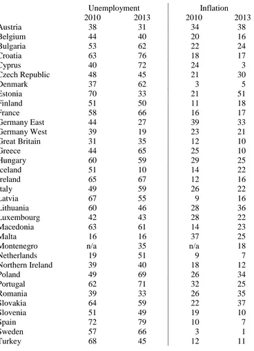
This is confirmed when investigating views and opinions regarding the most important problems in Europe – a type of analysis that closely resembles Shiller (1997). In two recent Eurobarometer surveys taken in May 2010 and May 20103 (#73.4 and #79.3 respectively) the overall proportion of respondents saying that unemployment was the most important problem was considerably higher than the proportion saying they were most worried about inflation (see Table 3). Indeed, in the perception of European citizens, unemployment exceeded inflation as the more important problem by a factor of around 2.5, and in several countries, including Denmark, Spain and Sweden by a factor of more than ten.

3. Trade-offs between unemployment and inflation

8

them. In 2004, the year in which they joined the EU, the A8 countries – the Czech Republic, Estonia, Hungary, Latvia, Lithuania, Poland, Slovakia and Slovenia – were added. Bulgaria and Romania also joined in that year, as did two further EU Candidate Countries - Croatia and Turkey. Data are available on Norway for 1990-1995 when it was an EU Candidate Country, and a member of the OECD. Overall, we make use of micro-data on over 1.1 million individuals from thirty one countries - Austria; Belgium; Bulgaria; Croatia; Cyprus; Czech Republic; Denmark; Estonia; Finland; France; Germany; Greece; Hungary; Iceland; Ireland; Italy; Latvia; Lithuania; Luxembourg; Malta; the Netherlands; Norway; Poland; Portugal; Romania; Slovakia; Slovenia; Spain; Sweden, Turkey and the UK. We then map in annual data on unemployment, inflation along with GDP growth for each country using Eurostat data.13

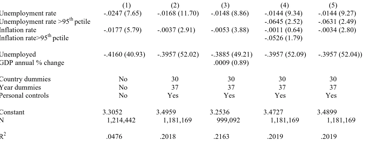
In Table 4a we estimate life satisfaction equations as in Equation 1 using OLS. It is clear that the direction of causation here runs from unemployment and inflation to well-being; the reverse causation is unlikely to be a major issue here. To deal with institutional factors which vary by country we include country fixed effects. To account for time varying factors we include year dummies.

The dependent variable is the 4-step life satisfaction question as reported in Section 1 (Q2).

Regressors include the inflation rate (i.e., the Harmonized Index of Consumer Prices or HICP) and the unemployment rate, which are both drawn from Eurostat. Column 1 includes only three variables – the unemployment and inflation rates and four labor force status dummies, although we only report the results on being unemployed. The excluded category is being employed. All the remaining equations in Table 4a include a full set of year and country dummies. Columns 2-5 also include a standard set of controls for gender, marital status, age, home-working, retired and being a student. In all cases the standard errors are clustered at the country*year level to overcome the problem of the common error component caused by the inclusion of country and year level variables in an individual-level regression. This is known as the Moulton (1986, 1991) standard-error problem which is fixed by clustering.

As expected, both the unemployment rate and the inflation rate have negative coefficients, suggesting that an increase in either lowers happiness; below we use these data to estimate the weighted misery ratio. Column 2 adds personal controls, which have little impact on our overall estimates. In all cases both the unemployment rate and the inflation rate are highly significant and negative. In addition the being unemployed dummy is also significantly negative with a t -statistic of around fifty. It appears that unemployment makes people very unhappy, which suggests it is unlikely to be voluntary. In column 3 annual GDP growth rates are added for a subset of countries to allow for business cycle effects but this variable is insignificant. Indeed, in no specification we tried was this variable ever found to be significant and hence was dropped. Column 4 adds dummy variables taking the value 1 if the inflation or unemployment rates were in the 95th percentile and zero otherwise. These are both negative and large. The unemployment

13 _{We have the following years of data by country - Belgium, Denmark, France, Germany, Ireland, Italy,}

9

term is significant while the inflation term is not, so it is omitted in column 5. It is high unemployment of over 19% that hurts. We also included a dummy variable for deflation, but this was never significant (results not reported).

In Table 4b we experiment with leads and lags on both unemployment rate and inflation. This can also be seen as test to potential simultaneity bias. Column 1 adds 1 year lags to current levels. Neither of the lags is significant. The same is true in the second column when we include two-period lags. In column 3 we include one year leads, to begin to capture the notion that future unemployment and inflation may affect current utility:only the term in future unemployment seems to influence current well-being. Neither inflation term is now significant. In column 4 we reintroduce current values of inflation and unemployment, but neither is significant. These estimates use OLS, which may be biased since the expectations in Equation 3 should reflect predicted rather than actual outcomes. Such predictions must be formed with information available to individuals in the current period. In column 5 we report an instrumental variable estimate based on this approach: the one-year-ahead variables, are instrumented by their current and past values. Again, it is only the unemployment variable that is significant.

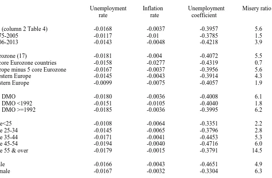
What do these estimates suggest about the relative size of the effects from the unemployment rate and the inflation rate? These are summarized in Table 5. The effects of unemployment and inflation, in row 1 of Table 5 - which is taken from column 2 of Table 4a - have coefficients of - 0.0168 and –.0037, respectively. These represent the effect upon well-being of a one percentage point change in each of the two independent variables. Following Di Tella et al (2001) – henceforth DMO – the implicit welfare-constant trade-off between inflation and unemployment can now be calculated. As in conventional economic theory, the DMO methodology leads to a measure of the marginal rate of substitution between inflation and unemployment – the slope of the indifference curve. This is analogous to the misery ratio, though it is weighted by the parameters α, β and (a transformation of) γ (see equation 1) and conditioned by the explanatory variables absent inflation and unemployment.

There are two consequences of unemployment – society as a whole becomes more fearful of unemployment (Blanchflower, 1991, Blanchflower and Shadforth, 2009, and Luechinger et al., 2010) and some people actually lose their jobs; there are aggregate and personal effects of unemployment. DMO argue that a way has to be found to measure the two unpleasant consequences of a rise in unemployment. DMO develop a way to take account of the extra cost of joblessness, namely, to calculate the sum of the aggregate and personal effects of unemployment. Our results are consistent with DMO (and the vast majority of works in happiness economics), who argue that a person who becomes unemployed experiences a larger reduction in wellbeing than the average individual. The loss from being unemployed, equals the coefficient on being ‘unemployed’ in a life-satisfaction micro regression. In column 2 of Table 4, this coefficient is -0.3957 and is highly statistically significant.

10

overall well-being cost of a one per cent increase in the unemployment rate. This can be interpreted as a combination of the direct effect of unemployment on well-being, plus the happiness costs associated with increased fear of unemployment and welfare interdependency effects on the associates of the unemployed.

Our results suggest that the well-being cost of a 1 percentage point increase in the unemployment rate equals the loss brought about by an extra 5.6 percentage points of inflation. How do we get this? The reason is that (0.0208/0.0037) = 5.6, where 0.0208 is the marginal unemployment effect on well-being, and 0.0037 is the marginal inflation effect on well-being from row 3 of column 2 of Table 4a. Hence 5.6 is the marginal rate of substitution between inflation and unemployment, conditional on the other explanatory variables. It is therefore our estimate of the weighted misery ratio based on individual data and correcting for individual characteristics. This is more than treble the 1.66 obtained by DMO. Note that DMO use three year rolling averages and adjust for omitted variable bias by running first stage micro life satisfaction equations in each country and year cell and then using the averaged residuals at the second stage of the regression. Using the micro data and adjusting the standard errors by clustering, the RHS variables by country and year accomplishes essentially the same adjustment. DMO do not make clear why they use three year rolling averages and we can see no compelling reasons to do so here; in any case this is unlikely to matter.

There is quite considerable variation in unemployment and inflation rates in the sample. However, the estimates cannot be generalized to every potential misery ratio. Hyperinflation scenarios are not part of stable economies analyzed in the paper.14 We are unable to determine whether our results would be the same if inflation were 1000% and unemployment was 4%, because the inflation data we have has a minimum of -4.5% (Ireland, 2009) and a maximum of 32.0% (Macedonia, 2010). We experimented with alternative specifications of the inflation rate to allow for the possibility that there are non-linear effects from inflation, including entering the inflation rate and its square and the square was never significant.

It is also possible to obtain estimates for sub-groups. Here we exclude the higher inflation term for simplicity and in part for sample size reasons. Table 5 shows that the misery ratio for 1975-2005 is much lower than it is over subsequent years (1.5 versus 3.9 respectively, noting of course that these are different than for the whole period, which arises from differences in the other coefficients). Western Europe has a higher elasticity than for Eastern Europe (4.3 and 21.9 respectively). Interestingly, the five core Eurozone countries - Germany, Austria, France, Finland, Netherlands and Austria – have an elasticity of 0.7 suggesting they fear inflation more than unemployment. Excluding these five ‘inflation hawk’ countries our elasticity estimate rises to 5.6. This estimate is in line with the textbook notion that individuals in the core countries of the Euro Area prefer "hard-nosed" governments (i.e. a governments which attach a lot of weight to fighting inflation), while the periphery has a predisposition for "wet governments" (i.e. governments which attach a higher weight to

14 _{Although, during the 20th Century there were quite a number of hyperinflationary events these can be put into}

11

fighting unemployment).15 We find evidence consistent with DMO for the years they looked at pre 1992 that the misery ratio is under two (1.8) but much higher since then for a consistent group of countries.

Females are more worried about unemployment than men (6.3 and 4.9 respectively). Conversely, the young put the greatest weight on inflation while the old put greater weights on unemployment.16 This runs counter to the evidence that entering the labor market during economic downturns has long term negative effects. Chances are these older folk have experienced unemployment and realize its lasting consequences. Unemployment hurts for a long time, especially long duration unemployment, which in the case of youngsters can cause permanent scars rather than temporary blemishes (Bell and Blanchflower, 2011a, 2011b). Older workers get over long spells of unemployment while youngsters don't, especially if they are unable to make an initial toe-hold in the labour market. However, when looking at the coefficients, the findings seem to be driven by the lower coefficient on inflation for the elderly. A possible potential explanation is that the elderly are more able to ensure that their assets (e.g. houses that they own) are less affected by inflation. We find strong evidence that unemployment lowers well-being markedly more than inflation does. Inflation rates above 25% do have especially large effects, as do unemployment rates of over 25%.

It is then feasible to obtain estimates for sub-groups. Here we exclude the higher inflation term for simplicity and in part for sample size reasons. Table 5 shows that the misery ratio for the EU27 is similar to that of the Euro Zone (3.7 and 3.8 respectively). Given such large sample sizes in every case the estimated ratios are significantly different from each other at conventional levels of significance. Western Europe has a higher elasticity than for Eastern Europe (4.39 and 2.0 respectively). Interestingly, the five core Eurozone countries - Germany, Austria, France, Finland, Netherlands and Austria – have an elasticity of 0.73 suggesting they fear inflation more than unemployment. Excluding these five ‘inflation hawk’ countries our elasticity estimate rises to 6.4. This estimate is in line with the textbook notion that individuals in the core countries of the Euro Area prefer "hard-nosed" governments (i.e. a governments which attach a lot of weight to fighting inflation), while the periphery has a predisposition for "wet governments" (i.e. governments which attach a higher weight to fighting unemployment).17 Females are more worried about unemployment than men (3.9 and 3.5 respectively). The least educated, the married, the widowed and the old are more concerned about unemployment – they put the highest weight on unemployment.

15 _{As a corollary, this result gives an indication of the possible tensions between the core and the periphery of the}

Euro Area; in this context it is of vital importance for the smooth functioning of the Eurosystem the institutional framework and by decision-making process of the European Central Bank

16 _{In contrast Lombardelli and Saleheen (2003) show that older people in the UK have higher expectations for}

inflation because they have experienced periods of higher inflation over their adult lives. They found that people in the age group 45–54 had experienced the highest level of inflation, an average inflation rate of 7.3% over their adult lives. They found that lifetime inflation experience has a significant effect on people’s inflation expectations.

17 _{As a corollary, this result gives an indication of the possible tensions between the core and the periphery of the}

12

The result that the old care most about unemployment is especially puzzling. It does not appear to be a function of the use of an age quadratic; the results are the same no matter how we specify the age variables in Table 4. We re-estimated all equations with single year of age dummies and the results were the same. The result that the old have a higher misery ratio is driven primarily by the lower coefficient for inflation for the elderly rather than any difference in the unemployment coefficient. An anonymous referee suggested that one factor that might drive this difference is house prices, in part because the old are more likely to own their own homes and don't mind higher inflation as it adds to their wealth. The opposite, of course, goes for the young who still have to buy their houses and hence suffer from higher inflation.

4. Discussion

Macroeconomic social welfare functions tend to focus on inflation and unemployment.18 The existence of a tradeoff between these variables allows central bankers to choose their short-run position on the Phillips curve. Starting from these premises, the fundament question for a central bank is to assign weights to unemployment and inflation to maximize social welfare. In other words, the central bank implicitly determines the marginal rate of substitution between inflation and unemployment. But our estimates of this quantity seem much higher than the implicit marginal rates of substitution held by most central banks. There are various reasons why this might be the case

One argument is that central banks implicitly or explicitly take the view that much of the variation in unemployment is due to changes in the natural rate, which are not susceptible to monetary policy intervention. This perhaps suggests higher frequency changes in the supply-side conditions of the labor market than many labor economists might expect. Nevertheless, since calibration of the natural rate may be problematic, this argument provides one possible rationale for central banks to focus monetary policy primarily on inflation. In our framework individuals cannot distinguish between a cyclical movement in unemployment and a change in the natural rate – both are equally costly in terms of well-being. Central banks may take a different view of the welfare implications of a change in unemployment depending whether they are believed to be the result of cyclical or structural changes in unemployment.

A second argument is based on our finding that the Phillips curve is rather steep. This finding derives from the following argument: our well-being regressions are static. There are clearly no dynamics associated with well-being, inflation or unemployment. We have therefore not taken account of the role of persistence in our estimates.19 There is a strand of the well-being literature relating to persistence. Clark et al. (2001), use panel data to investigate whether an individual’s past unemployment affect their current well-being. They show that unemployment “reduces the well-being of those who are currently in work: for them, past unemployment scars” Clark et al. (2001, p. 237).20 A similar argument is made for inflation; Blanchflower (2007) shows that “An

18

Frequently unemployment is replaced with output. This rests on the assumption that there is a stable relation between the loss in output production and unemployment as postulated by the Okun Law.

19 _{We are grateful to a referee for this point.}

20 _{A similar conclusion is reached by Knabe and Rätzel (2011); in their analysis, people who have experienced}

13

individual who has experienced high inflation in the past has lower happiness today, even holding constant today’s inflation and unemployment rates”. There is evidence of persistence at the individual level, which is dependent on the availability of panel data.

There is, however, another approach to persistence in macroeconomics where findings derive principally from time series results or calibration. Consider a Keynesian model, where the central bank objective is to minimise a quadratic loss function subject to a linear Phillips curve.

𝑚𝑖𝑛1₂{𝛼𝜋𝑡2+𝛽𝑢𝑡2}

𝑠.𝑡. : 𝑘𝜋𝑡+𝑢𝑡 = 0

Where 𝜋_𝑡 and 𝑢_𝑡 are inflation and unemployment at time t, respectively. k is the slope of the Phillips curve, which measures the response of inflation with relation to cyclical unemployment. 𝛼 and 𝛽 are the parameters indicating the weights that the central bank assign to inflation and unemployment. The first order condition yields the following solution:

𝑢𝑡 𝜋𝑡 =

𝛼 𝛽𝑘

Our estimates of 𝛼 and 𝛽 give a value for their ratio of 0.26 (this is equal to 1/3.76). The sample average for 𝑢 and 𝜋 over our sample period give 𝑢𝑡

𝜋𝑡= 1.9. This implies that the sacrifice ratio (-k) is

equal to -0.14 and that the Phillips curve is rather steep with a gradient = -7.14..21 22 This suggests a labour market with few and weak rigidities; prices respond quickly to movements in aggregate demand. Following from this finding, one might argue that the central bank does not need to be particularly responsive to the unemployment rate because, with such a steep Phillips curve, average durations are likely to be short if aggregate demand is relatively volatile.

A third argument takes our fining in relation to the Phillips curve in a somewhat different direction which focuses on the dynamics of the relationships, rather than focussing on the static framework that we have used thus far. Thus, consider the role of persistence by restating Equation 1 in more general dynamic form:

(2) 𝑈𝐶𝑡𝑖 =𝛼𝐸 � 𝛿𝑡𝑈𝑛𝑒𝑚𝑝𝑙𝑜𝑦𝑚𝑒𝑛𝑡𝐶𝑡𝑖

∞

𝑡=0

+𝛽𝐸 � 𝛿𝑡_{𝐼𝑛𝑓𝑙𝑎𝑡𝑖𝑜𝑛}

𝐶𝑡𝑖 + 𝛿𝜴𝑐𝑡𝑖 + 𝛾𝑐 + 𝜂𝑡 + 𝜇𝑐𝑡𝑖 ∞

𝑡=0

21 _{We thank T.S. Fuerst for this point.}

22

14

The left hand side variable, U, now corresponds more closely to the conventional macroeconomic understanding of utility. The right hand side includes expected future levels of inflation and unemployment, discounted at the rate δ, as well as their current levels. The remaining terms are identical to those in Equation (1), without loss of generality. The “being unemployed” variable is subsumed within the unemployment variable, without affecting the argument. This specification tries to more closely represent the problem faced by the central bank, which might be characterised as seeking to maximize the present value of aggregate utility rather than focussing simply on its current level. This allows for the possibility that, at the individual level, the future may be regarded with positive or negative anticipation.

We already know that the past matters. Past events are part of the information set that determines current well-being and there is evidence of the persistence of the effects of past unemployment and inflation on current well-being. But there is no evidence from individual surveys of the effect of expected unemployment and inflation on current well-being. Any such impact will also clearly depend on the rate at which the future is discounted.

Omitting future expectations from our specification could therefore have led to bias in the results we presented in Table 4a. What might be the extent of this bias? To keep the analysis simple, assume that both unemployment and inflation follow AR(1) processes. After some simple manipulation, one can show that the relationship between our estimates and the “true” value of the marginal rate of substitution is given by:

(3) 𝛼

𝛽= 𝛼� 𝛽�

(1−𝛿𝜌𝑈)

(1−𝛿𝜌𝜋)

where ρU and ρπ are, respectively, the coefficients associated with the AR(1) processes in

unemployment and inflation and the estimated coefficients from Equation (1) are 𝛼� and 𝛽̂. Equation (3) shows that the modification to the estimated ratio from Equation (1) depends on the relative degree of persistence (size of the AR(1) coefficient) in unemployment and inflation. If unemployment is substantially more persistent than inflation, then the estimated marginal rate of substitution from cross-sectional data may be upward biased. This bias also increases with the discount rate.

To investigate these issues, we estimated AR(1) coefficients from annual unemployment and inflation data which were measured consistently by Eurostat for the period 1996-2012. Our estimate of the AR(1) unemployment coefficient ρU was 0.815 and for the AR(1) inflation

15

households, he estimates discount factors below 0.95. Gourninchas and Parker (2002) find estimates of about 0.93 for the general population.

The value of α/β in Equation (3) then solves to 1.63. Thus, if this model of forward expectations is valid, the marginal rate of substitution is substantially reduced, though still greater than unity, and though the central bank would pay more attention to inflation, the implication of the results would still be that unemployment be given a greater weight. Of course, any reduction in the discount rate below 0.99 would increase this weight further and, in the limit when δ = 0, the marginal rate of substitution would return to 5.6. Nevertheless, taking account of dynamics seems to result in a lower estimate of the marginal rate of substitution and provides another rationale for central banks, and the politicians who design their objective function, giving less weight to unemployment than our static estimates of the tradeoff between unemployment and inflation might suggest.

There are arguments for not pressing this persistence model too strongly. First, it does not in any way disaggregate the population: we know already that responses to unemployment and inflation differ across populations. Such heterogeneity may lead to aggregation bias. There is also evidence that discount rates vary across groups (Carroll, 1997 and Liabson et al., 2003). For example, our populations have finite lives, which suggest that there should either be an upper limit on the future number of time periods in (3) or a more complex overlapping generations structure. In both these formulations, for example, one would expect older agents to discount the future more heavily.

These three arguments – natural rate variation, steepness of the Phillips curve and differences in persistence - provide useful qualifications to our simple static results. They suggest reasons why the central bank’s implicit preference orderings do not directly reflect those of individuals based on static survey analyses. Perhaps, paraphrasing Knabe and Rätzel (2011), unemployment not only scars individuals but also scares them. Although it is not possible to provide a clear explanation of the reason underlining these differences between theory and surveys, Sapienza and Zingales (2013, p. 642) show that “economic experts seem to provide answers very different than those of average” individuals. This is consistent with our argument that the central bank may choose to focus on inflation even though the public would prefer it to concentrate on unemployment because it has access to a wider information set than most individuals. It may implicitly also have lower rates of time preference, which would imply giving greater attention to arguments involving the dynamics of inflation and unemployment.

16

degree of heterogeneity exists within the Euro-area, is that a gradualist disinflationary policy is likely to be more desirable from a welfare point of view.

5. Conclusions

During the last three decades theory and practice of central banking have witnessed a remarkable convergence throughout the world. The pre-crisis consensus was that a conservative central bank and an inflation target (or reference value) was all that was required for a central bank to gain credibility and ultimately to maximize social welfare. After the Great Recession, this consensus has been challenged and from many parts of the society it is increasingly seen as inadequate.

Our paper contributes to the literature on the trade-off between unemployment and inflation. The approach differs substantially from the standard macroeconomic modelling. We make use of a large European dataset, covering the period 1975 to 2013, to estimate happiness equations in which an individual subjective measure of life satisfaction is regressed against unemployment and inflation rate (controlling for personal characteristics, country and year fixed effects). We interpret the coefficients on unemployment and inflation as implicit weights on a subjective welfare function. We compute a weighted misery ratio that can be interpreted as the trade-off between inflation and unemployment that will leave people, on average, equally happy. The main results of this paper can be summarized as follows:

• Unemployment lowers happiness of the unemployed but also the happiness of everyone else.

• We estimate the unemployment/inflation trade-off as approximately 5.6, when the whole sample is used. That is to say a 1 percentage point increase in unemployment lower well-being nearly six times more than an equivalent rise in inflation. Using only the five main euro area countries that are especially worried about inflation – Germany, Austria, France, Finland and Austria – the elasticity decreases to one.

• We find that , women and, somewhat surprisingly, the old put the highest weight on unemployment

Our results using survey data depart from the more common finding in the macroeconomic literature which puts more weight on inflation rather than on unemployment. In order to investigate this further, we have analyzed the role of persistence using a simple model of forward expectations. The marginal rate of substitution is substantially reduced, though still greater than unity, and though the central bank would pay more attention to inflation, the implication of the results would still be that unemployment be given a greater weight.

17

18 References

Alesina, A, R. Di Tella and R.J. MacCullough (2004), 'Inequality and happiness: are Europeans and Americans different?', Journal of Public Economics, 88, pp. 2009-2042.

Bailey, M. J. (1956), 'The welfare cost of inflationary finance,' Journal of Political Economy, 64(2), pp 93-110.

Banks, J., M. Marmot, Z. Oldfield and J.P. Smith (2006), 'Disease and disadvantage in the United States and England', Journal of the American Medical Association, 295, pp. 2037-2045.

Barro, R.J., (1976), 'Rational expectations and the role of monetary policy,' Journal of Monetary Economics, Elsevier, 2(1), pp. 1-32, January.

Bell, D.N.F , and D.G. a (2011a), 'Young people and the Great Recession', Oxford Review of Economic Policy, 27: pp. 241-267.

Bell, D.N.F, and D.G. Blanchflower (2011b), 'Youth unemployment in Europe and the United States', Nordic Economic Policy Review, 1, pp. 11-38.

Benabou, R. and R. Gertner (1993), 'Search with learning from prices: does increased inflationary uncertainty lead to higher markups?,' Review of Economic Studies, 60(1), pp. 69-94, January.

Blanchflower D.G. (1991), 'Fear, unemployment and pay flexibility', Economic Journal, 101(405), May, pp. 483-496.

Blanchflower D.G. (2007a), 'International evidence on well-being', in Measuring the subjective well-being of nations: national accounts of time-use and well-being, edited by Alan B. Krueger, NBER and University of Chicago Press.

Blanchflower D.G. (2007b), 'Is unemployment more costly then inflation?", NBER Working Paper W13505, October.

Blanchflower D.G. and C. Shadforth (2009) 'Fear, unemployment and migration,' Economic Journal, 2009, 119(535), February, F136-F182

Blanchflower, D.G., N. Christakis and A.J. Oswald (2011), 'An introduction to the structure of biomarker equations', mimeo, December.

Blanchflower D.G. and A.J. Oswald (2004), 'Well-being over time in Britain and the USA', Journal of Public Economics, 88, pp. 1359-1386.

19

Blanchflower D.G. and A.J. Oswald (2005), 'Happiness and the Human Development Index: the paradox of Australia,' Australian Economic Review, 2005, 38(3), 307-318, September.

Blanchflower D.G. and A.J. Oswald (2011), 'International happiness: a new view on the measure of performance', Academy of Management Perspectives, February, 25(1), pp. 6-22.

Blanchflower D.G. and C. Shadforth (2009), 'Fear, unemployment and migration', Economic Journal, 119(535), February, F136-F182.

Carroll, C.D. (1997). 'Buffer Stock Saving and the Life Cycle/Permanent Income Hypothesis,' Quarterly Journal of Economics, Vol. CXII(1), February, pp. 1-57.

Carroll, C.D. and A.A. Samwick (1997), ‘The nature of precautionary wealth,’ Journal of Monetary Economics, vol. 40(1), pp. 41-71, September.

Clark, A.E., Diener, E., Y. Georgellis and R.E. Lucas (2008), 'Lags and leads in life satisfaction: a test of the baseline hypothesis', Economic Journal, 118: F222–F243.

Clark, A.E., Y. Georgellis and P. Sanfey (2001), 'Scarring: the psychological impact of past unemployment,' Economica, 68(270), pp. 221-41, May.

Deaton, A. (2008), 'Income, health and wellbeing around the world: evidence from the Gallup World Poll', Journal of Economic Perspectives, 22(2), pp. 53-72.

Di Tella R. MacCulloch R.J. and A.J. Oswald (2001), 'Preferences over inflation and unemployment: evidence from surveys of happiness', American Economic Review, 91, pp. 335- 341.

Di Tella, R.J. MacCulloch, and A.J. Oswald (2003), 'The macroeconomics of happiness,' Review of Economics and Statistics, 85 (4), November, pp. 793–809.

Di Tella R., R.J. MacCulloch R.J., (2006), 'Some uses of happiness data in economics,' Journal of Economic Perspectives, 20(1), pp. 25-45.

Easterlin, R. (1974), 'Does economic growth improve the human lot? Some empirical evidence', in Nations and households in economic growth, essays in honor of Moses Abramowitz, David, P.A., Reder, M.W. (editors), Academic Press, New York.

Easterlin R.A. (2003), 'Explaining happiness', Proceedings of the National Academy of Sciences, 100, pp. 11176-11183.

Ekman, P., R. Davidson and W. Friesen (1990), 'The Duchenne smile: emotional expression and brain physiology II', Journal of Personality and Social Psychology, 58(2), pp. 342–53.

20

Ferrer-i-Carbonell, A., and P. Frijters, (2004), 'How important is methodology for the estimates of the determinants of happiness?', Economic Journal, 114(July), pp. 641-659.

Frijters, P., Johnston, D. W. and Shields, M. A. (2011), 'Life satisfaction dynamics with quarterly life event data', Scandinavian Journal of Economics, 113, pp. 190–211.

Frey B.S. and Stutzer A. (2002), 'What can economists learn from happiness research?', Journal of Economic Literature, 40(2), June, pp. 402-435.

Friedman, M. (1971), ‘Government revenue from inflation,’ Journal of Political Economy, pp. 846-856.

Gardner, J. and A.J. Oswald (2007), 'Money and mental well-being: a longitudinal study of medium sized lottery wins', Journal of Health Economics, 26, pp. 49-60.

Gilbert D. (2006), Stumbling on happiness, Alfred A Knopf: New York.

Gourinchas, Pierre-Olivier and Jonathan A. Parker (2002), 'Consumption over the life cycle,' Econometrica, January, 70(1), 47-89.

Graham, C. (2010), Happiness around the world. the paradox of happy peasants and miserable millionaires, Oxford University Press

Graham, C. (2011), The Pursuit of Happiness: An Economy of Well-Being, Brookings Institution Press.

Heinz, W. (2007), 'Macroeconomics and life satisfaction: revisiting the misery index', Journal of Applied Economics, X(12), pp. 237-251.

Heinz, W. (2010), 'The magic triangle of macroeconomics: how do European countries score?', Oxford Economic Papers, pp. 1-23.

Kahneman D., Krueger A.B., Schkade D., Schwarz N., Stone A.A. (2004), 'Toward national wellbeing accounts', American Economic Review Papers and Proceedings, May, 94, pp. 429-434.

Krueger, A.B. (2009), 'Comments on "Happiness, contentment, and other emotions for central bank policymakers"' by Rafael Di Tella and Robert MacCulloch' in Policymaking Insights from Behavioral Economics, C.L. Foote, L. Goette, and S. Meier (editors), Federal Reserve Bank of Boston.

Layard, R. (2011), Happiness, Lessons From a New Science, Penguin 2nd edition.

21

Laibson, David, Andrea Repetto, and Jeremy Tobacman (2003) 'A debt puzzle,' in Knowledge, information and expectations in modern macroeconomics: in honor of Edmund S. Phelps, Philippe, A., R. Frydman, J.Stiglitz, and M. Woodford (editors), Princeton University Press: Princeton, N.J..

Lombardelli, C. and J. Saleheen (2003), ‘Public expectations of UK inflation’, Quarterly Bulletin, Bank of England, Autumn, pp. 281-290.

Lucas Jr, R. E. (2000), ‘Inflation and welfare’, Econometrica, 68(2), pp 247-274.

Lucas, E., Clark A.E., Georgellis Y., Diener E. (2004), 'Unemployment alters the set point for life satisfaction', Psychological Science, 15 (1), pp. 8-13.

Luechinger, S., Meier, S., and Stutzer, A. (2010), 'Why does unemployment hurt the employed? Evidence from the life satisfaction gap between the public and the private sector,' Journal of Human Resources, 45(4), pp. 998-1045.

Luttmer, E. (2005), 'Neighbors as negatives; relative earnings and well-being', Quarterly Journal of Economics, 120(3), pp. 963-1002, August.

Mackerron, G. (2012), ‘Happiness economics from 35,000 feet’, Journal of Economic Surveys 26(4), pp. 705–735, September 2012.

Moulton, B.R. (1986), 'Random group effects and the precision of regression estimates', Journal of Econometrics, 32, pp. 385-397.

Moulton, B.R. (1991), 'An illustration of a pitfall in estimating the effects of aggregate variables on micro units', Review of Economics and Statistics, 72, pp. 334-8

Oswald, A. J., and S. Wu (2010), ‘Objective confirmation of subjective measures of human well-being: evidence from the USA,’ Science, 327, pp. 576–579.

Powdthavee, N. (2010), The Happiness Equation, Duxford, UK: Icon Books

Rotemberg, Julio J and Michael Woodford (1998), ‘An optimisation-based econometric framework for the evaluation of monetary policy’, in NBER Macroeconomics Annual, Ben S Bernanke and Julio J. Rotemberg (eds), pp 297-346.

Ruprah I.J. and Luengas P. (2011), ‘Monetary policy and happiness: preferences over inflation and unemployment in Latin America’, The Journal of Socio-Economics, 40, pp. 59-66.

Samwick, A.A. (1998), ‘Discount rate heterogeneity and social security reform,’ Journal of Development Economics, vol. 57(1), pp. 117-146, October.

22

Shiller, R. J. (1997), ‘Why do people dislike inflation?' In Reducing Inflation: Motivation and Strategy, Christine Romer and David H. Romer (editors), University of Chicago Press.

Ubel P.A., Loewenstein G, Jepson C. (2005), 'Disability and sunshine: can hedonic predictions be improved by drawing attention to focusing illusions or emotional adaptation?', Journal of Experimental Psychology: Applied, 11, pp. 111-123.

Wolfers, J. (2003), 'Is business cycle volatility costly? Evidence from surveys of subjective well-being', International Finance, 6:1, pp. 1-26.

Wolfers, J. and A. Leigh (2006), 'Happiness and the Human Development Index: Australia is not a paradox', Australian Economic Review, 39(2), June, pp. 176-184.

23 Table 1. European Misery Ratio

Misery Ratio 1975-1979 1980-1989 1990-1999 2000-2010

Belgium 0.76 2.46 4.26 4.34

Denmark 0.68 1.31 3.68 2.29

Finland 1.30 10.30 4.69

France 0.43 2.38 4.85 5.19

Germany 0.92 0.40 2.50 5.43

Greece 1.81 0.76 3.07

Ireland 0.66 1.03 5.10 1.80

Italy 0.44 0.30 2.57 3.84

Luxembourg 0.07 4.15 0.77 1.16

Netherlands 0.78 0.54 2.38 1.35

Portugal 0.72 2.39

Spain 4.09 4.15

UK 0.29 1.56 2.23 3.14

Source: Eurostat

Table 2. Unemployment and HCIP inflation rate October 2013 and Misery ratios

Unemployment rate Inflation rate Absolute Misery ratio

Austria 4.8 2.3 2.1

Belgium 9.0 1.4 6.4

Bulgaria 13.2 1.0 13.2

Cyprus 17.0 0.8 21.3

Czech Republic 6.8 1.6 4.3

Denmark 6.7 0.8 8.4

Estonia 8.8 3.5 2.5

Finland 8.1 2.5 3.2

France 10.9 1.1 9.9

Germany 5.2 1.7 3.1

UK 7.5 2.1 3.6

Greece 27.3 -0.4 68.3

Hungary 17.6 2.5 7.0

Ireland 12.6 0.7 18.0

Italy 12.5 1.6 7.8

Latvia 11.9 0.3 39.7

Lithuania 11.1 1.6 6.9

Luxembourg 5.9 1.9 3.1

Malta 6.4 1.4 4.6

Netherlands 7.0 2.9 2.4

Poland 10.2 1.1 9.3

Portugal 15.7 0.8 19.6

Romania 7.3 3.7 2.0

Slovakia 13.9 2.0 7.0

Slovenia 10.1 2.2 4.6

Spain 26.7 2.0 13.4

Sweden 7.9 0.5 15.8

24 Table 3. Views on Unemployment and Inflation

Unemployment Inflation 2010 2013 2010 2013

Austria 38 31 34 38

Belgium 44 40 20 16

Bulgaria 53 62 22 24

Croatia 63 76 18 17

Cyprus 40 72 24 3

Czech Republic 48 45 21 30

Denmark 37 62 3 5

Estonia 70 33 21 51

Finland 51 50 11 18

France 58 66 16 17

Germany East 44 27 39 33

Germany West 39 19 23 21

Great Britain 31 35 12 10

Greece 44 65 25 10

Hungary 60 59 29 25

Iceland 51 10 14 22

Ireland 65 67 12 16

Italy 49 59 26 22

Latvia 67 55 9 16

Lithuania 60 46 28 36

Luxembourg 42 43 28 22

Macedonia 63 61 14 23

Malta 16 16 37 25

Montenegro n/a 35 n/a 18

Netherlands 19 51 9 7

Northern Ireland 39 40 18 12

Poland 49 69 26 34

Portugal 62 71 32 25

Romania 39 33 26 35

Slovakia 64 59 22 37

Slovenia 51 49 19 10

Spain 72 79 10 7

Sweden 57 66 3 1

Turkey 68 45 12 11

Source: Eurobarometers #73.4 May 2010 & #79.3 May 2013

25

Table 4a. Life satisfaction, unemployment and inflation in 31 European countries, 1975-2013

(1) (2) (3) (4) (5) Unemployment rate -.0247 (7.65) -.0168 (11.70) -.0148 (8.86) -.0144 (9.34) -.0144 (9.27)

Unemployment rate >95th pctile -.0645 (2.52) -.0631 (2.49)

Inflation rate -.0177 (5.79) -.0037 (2.91) -.0053 (3.88) -.0011 (0.64) -.0034 (2.80)

Inflation rate>95th pctile -.0526 (1.79)

Unemployed -.4160 (40.93) -.3957 (52.02) -.3885 (49.21) -.3957 (52.09) -.3957 (52.04))

GDP annual % change .0009 (0.89)

Country dummies No 30 30 30 30

Year dummies No 37 37 37 37

Personal controls No Yes Yes Yes Yes

Constant 3.3052 3.4959 3.2536 3.4727 3.4899

N 1,214,442 1,181,169 999,092 1,181,169 1,181,169

R2 .0476 .2018 .2163 .2019 .2019

26

Table 4b. Life satisfaction, unemployment and inflation with leads and lags in 31 European countries, 1975-2013

(1) (2) (3) (4) (5)

OLS OLS OLS OLS IV

Unemployment ratet -.0197 (5.39) -.0111 (3.00) -.0049 (1.49) -.0031(0.49) Unemployment ratet-1 .0036 (1.02) .0004 (0.11) -.0007 (0.19)

Unemployment ratet-2 -.0048 (1.57)

Unemployment ratet+1 -.0102 (2.92) -.0112 (2.74) -.0149 (7.96)

Inflation ratet -.0081 (2.76) -.0063 (2.02) -.0036 (1.26) -.0059 (1.50)

Inflation ratet-1 .0026 (1.01) -.0024 (0.75) .0011 (0.46)

Inflation ratet-2 .0023 (0.89)

Inflation ratet+1 -.0030 (1.00) -.0019 (0.64) -.0026 (1.69)

Unemployed -.3825 (42.83) -.3815 (37.58) -.3747 (40.39) -.3782 (38.36) -.3969 (48.19)

Country dummies 30 30 30 30 30

Year dummies 36 37 37 37 37

Constant 3.2328 3.2202 3.4727 3.2468 3.5629

N 999,497 866,397 983,694 945,409 1,080,168

R2 .1886 .1886 .1869 .1824 .1969

27 Table 5. Estimates of the weighted misery ratio

Unemployment Inflation Unemployment Misery ratio rate rate coefficient

All (column 2 Table 4) -0.0168 -0.0037 -0.3957 5.6

1975-2005 -0.0117 -0.01 -0.3785 1.5

2006-2013 -0.0143 -0.0048 -0.4218 3.9

Eurozone (17) -0.0181 -0.004 -0.4072 5.5

5 core Eurozone countries -0.0158 -0.0277 -0.4319 0.7

Europe minus 5 core Eurozone -0.0167 -0.0037 -0.3956 5.6

Western Europe -0.0145 -0.0043 -0.3914 4.3

Eastern Europe -0.0099 -0.0075 -0.4057 1.9

All DMO -0.0180 -0.0036 -0.4008 6.1

All DMO <1992 -0.0151 -0.0105 -0.4040 1.8

All DMO >=1992 -0.0185 -0.0036 -0.3995 6.2

Age<25 -0.0108 -0.0064 -0.3351 2.2

Age 25-34 -0.0145 -0.0065 -0.3796 2.8

Age 35-44 -0.0171 -0.0041 -0.4453 5.3

Age 45-54 -0.0194 -0.0040 -0.4716 6.0

Age 55 & over -0.0179 -0.0015 -0.3791 14.5

Male -0.0166 -0.0043 -0.4651 4.9

Female -0.0167 -0.0032 -0.3304 6.3