promoting access to White Rose research papers
White Rose Research Online
[email protected]
Universities of Leeds, Sheffield and York
http://eprints.whiterose.ac.uk/
This is a copy of the final published version of a paper published via gold open access
in
Genetic Epidemiology
.
This open access article is distributed under the terms of the Creative Commons
Attribution Licence (http://creativecommons.org/licenses/by/3.0), which permits
unrestricted use, distribution, and reproduction in any medium, provided the
original work is properly cited.
White Rose Research Online URL for this paper:
http://eprints.whiterose.ac.uk/84363
Published paper
Genetic
Epidemiology
R
ESEARCH
A
RTICLE
Novel Bayes Factors That Capture Expert Uncertainty
in Prior Density Specification in Genetic Association
Studies
Amy V. Spencer,1Angela Cox,2Wei-Yu Lin,2,3Douglas F. Easton,4,5Kyriaki Michailidou,4and Kevin Walters1∗
1School of Mathematics and Statistics, University of Sheffield, Sheffield, UK;2Department of Oncology, Sheffield Cancer Research Centre,
University of Sheffield Medical School, Sheffield, UK;3Department of Neurosurgery, Chang Gung Memorial Hospital, Taoyuan County, Taiwan; 4Department of Public Health and Primary Care, Centre for Cancer Genetic Epidemiology, University of Cambridge, Cambridge, UK;5Department of
Oncology, Centre for Cancer Genetic Epidemiology, University of Cambridge, Cambridge, UK
Received 18 March 2014; Revised 21 October 2014; accepted revised manuscript 5 November 2014.
Published online in Wiley Online Library (wileyonlinelibrary.com). DOI 10.1002/gepi.21891
ABSTRACT: Bayes factors (BFs) are becoming increasingly important tools in genetic association studies, partly because they provide a natural framework for including prior information. The Wakefield BF (WBF) approximation is easy to calculate
and assumes a normal prior on the log odds ratio (logOR) with a mean of zero. However, the prior variance (W) must be
specified. Because of the potentially high sensitivity of the WBF to the choice ofW, we propose several new BF approximations
with logOR∼N(0,W), but allowW to take a probability distribution rather than a fixed value. We provide several prior
distributions forWwhich lead to BFs that can be calculated easily in freely available software packages. These priors allow a
wide range of densities forWand provide considerable flexibility. We examine some properties of the priors and BFs and show
how to determine the most appropriate prior based on elicited quantiles of the prior odds ratio (OR). We show by simulation
that our novel BFs have superior true-positive rates at low false-positive rates compared to those from bothP-value and WBF
analyses across a range of sample sizes and ORs. We give an example of utilizing our BFs to fine-map the CASP8region
using genotype data on approximately 46,000 breast cancer case and 43,000 healthy control samples from the Collaborative Oncological Gene-environment Study (COGS) Consortium, and compare the single-nucleotide polymorphism ranks to those
obtained using WBFs andP-values from univariate logistic regression.
Genet Epidemiol 00:1–10, 2015. Published 2015 Wiley Periodicals, Inc.∗
KEY WORDS:expert knowledge; elicitation; sensitivity; hyperparameter; flexibility; single-nucleotide polymorphism; filtering; empirical; fine mapping
Introduction
Recently, several methods have been published for analyzing genotype data at the fine-mapping level [Maller et al., 2012; Udler et al., 2009; Vignal et al., 2011]. These data consist of hundreds or thousands of single-nucleotide polymorphisms (SNPs) in a small region of the genome, where associations with a disease have previously been found, commonly in a genome-wide association study (GWAS). Bayesian methods [Stephens and Balding, 2009] have the advantage of naturally allowing for the inclusion of prior functional genetic infor-mation which could inform the probability of an SNP being causal. This could help to overcome the problems faced in fine-mapping, where it is expected that the causal SNPs not yet identified are likely to have small effect sizes (odds ratios [ORs] of the order of 1.1 or less) and the results are likely to be confounded by high levels of short-range linkage disequi-librium (LD). Furthermore, some causal SNPs may have low minor allele frequencies (MAFs). These factors make it diffi-cult to identify causal SNPs, even using the tens of thousands
Supporting Information is available in the online issue at wileyonlinelibrary.com. ∗Correspondence to: Kevin Walters, School of Mathematics and Statistics,
Univer-sity of Sheffield, Sheffield, S3 7RH, UK. E-mail: [email protected]
of subjects that are currently being analyzed by international consortia.
We previously carried out a thorough investigation of several different frequentist fine-mapping filtering methods [Spencer et al., 2014]. Filtering is a general framework in which the SNPs are ranked according to a given statistic, a threshold value of that statistic is chosen and SNPs with a value below this threshold are removed from the set of candidate causal SNPs. This results in a more manageable number of SNPs which can be investigated for causality in further biological tests, such as the analysis of gene expres-sion in cell lines. The Bayes factor (BF) is a Bayesian statistic which can be used for filtering [Kass and Raftery, 1995], and it has already been used as a tool for use in genetic associa-tion analyses [Stephens and Balding, 2009; Wakefield, 2008, 2009]. The calculation of BFs is now implemented in genetic analysis software such as SNPTEST2 [Marchini et al., 2007] and
their use is becoming increasingly popular as a filter in fine-mapping studies [Maller et al., 2012]. The BF is a ratio, which compares the probabilities of the data under two models or hypotheses. In this setting, they compare two models, one in which an SNP is not causally associated with a disease and the other in which it is. They can be used alone or used to
C
update prior odds of the SNP being causal. BFs often have to be approximated due to intractable integrals and, although current methods of approximation are good, they restrict the form of the prior on the effect size.
We consider the use of Wakefield’s approximate BF [Wake-field, 2008, 2009], which requires that each SNP has a prior on its log odds ratio (logOR) of the formN(0,W) for some fixedW. When eliciting a value ofWfrom experts it may be the case that there is some uncertainty inW, perhaps because several quantiles have been elicited giving inconsistent values ofW. Because of this we examine several families of prior distributions onW, which result in novel tractable BFs. Such priors onWcan be thought of as providing a weighted average of the BF over each value in the support ofW. We examine the properties of these priors onWand give the novel BF approximations in forms that are easily calculable in com-monly used software. Although this removes the problem of specifying a fixedW value, most of the novel BFs require hyperparameters to be specified. We demonstrate how ap-propriate values may be obtained via expert elicitation.
The BFs we describe could be used in any genetic asso-ciation study, but we give an example with simulated fine-mapped data to show how effective the use of these BFs can be in filtering. We compare the results to those using the Wakefield BF (WBF) and examine the effect of the choice of hyperparameters. We give an example of eliciting the prior hyperparameters and using the BFs as a fine-mapping tool using breast cancer case-control data from an international consortium. We are able to show that our methods may be used to describe a variety of uncertainties and appropriately incorporate these into a BF analysis. Not only this, but they can potentially produce better results than if the uncertainty was not taken into account.
Materials and Methods
Bayes Factors and the Wakefield Approximation
BFs compare the probability of the observed data under two models or hypotheses. For our purposes, the BF can be defined as
BF= P(data|H1)
P(data|H0)
. (1)
BFs are also used to update prior odds (δ/(1–δ)) to posterior odds (/(1–)) via /(1–)=δ/(1–δ)×BF, where in our caseandδ are the posterior and prior probabilities of “true” association, respectively. By “true association,” we mean causally linked to disease risk rather than being asso-ciated through LD or sampling variation. Here, a BF greater than one indicates that the data are more likely under the alternative than the null hypothesis. BFs require the specifi-cation of a likelihood and prior on all model parameters. Both BFs and posterior probabilities can be used to fine-map ge-nomic regions in case-control studies by using the likelihood from a logistic regression model. For SNPiin single-SNP
logistic regression models, the probability (yij) of subjectj,
withxij copies of the minor allele, being a case is
yij =
eβ0i+β1ixij
1+eβ0i+β1ixij. (2) With this definition,β1ican be interpreted as the SNP-specific
per-allele natural logarithm of the OR comparing the minor to the major allele. For SNPi, BFi is calculated comparing
the hypothesesH0:β1i=0 andH1:β1i=0 [Stephens and
Balding, 2009].
The BF, as given in Equation (1), is the ratio of marginal likelihoods which can lead to intractable integrals for many prior densities. For nontractable BFs, it is common to use a Laplace approximation [Kass and Raftery, 1995]. The Laplace approximation is implemented in software packages, includ-ing SNPTEST2 [Marchini et al., 2007]. Wakefield [2008, 2009] derived a tractable approximation to the BF (which we ab-breviate as WBF). We found excellent agreement between the WBF and Laplace approximations from SNPTEST2 for
sam-ple sizes≥10,000 for a variety of ORs and MAFs (data not shown). Both methods are based on asymptotic approxima-tions and, given the large sample sizes in the types of dataset we consider, should provide accurate approximations to the true BF.
Using the definition of the BF in Equation (1), the Wake-field approximate BF is
WBF=
V V+Wexp
β1 2
W 2V(V+W)
. (3)
In Equation (3), β1, the logOR of causal SNPs in the
ge-nomic region under consideration, is assumed to follow a normal distribution given byβ1∼N(0,W).β1is the
maxi-mum likelihood estimator (MLE) ofβ1. Rather than consider
the logistic likelihood, Wakefield used the asymptotic distri-bution of the MLE:β1∼N(β1,V) which leads to the WBF
given in Equation (3). Note that the WBF we specify in Equa-tion (3), and use in the rest of this paper, is the reciprocal of the WBF given by Wakefield [2009].
Motivation for the Study
To use the WBF, one needs to specifyW (e.g., through elicitation) and be prepared to accept that the prior distri-bution of the logOR is Gaussian. For a percentileβ1,p, such
thatp(β1<β1,p|β1∼N(0,W))=p,W is calculated using
W=β1,p/–1(p) 2
, whereis the distribution function of the standard normal distribution (Wakefield, 2009). When performing elicitation aboutWwith an expert, they may ex-press some uncertainty about the value ofW. For example, the expert may believe that the 80th percentile of the prior distribution for the OR is between 1.05 and 1.3 which implies that 0.003≤W≤0.1. As a result, we investigated how sensi-tive the WBFs are to the choice ofW. We found the results to be highly dependent on the choice ofW. We therefore wanted to allow for uncertainty aboutWin the BF calculations. We retained the normal density for the prior forβ1and
consid-ered three different parametric families of priors forWthat
Table 1. Prior densities forW
Name of prior f(W)∝ Restrictions on hyperparameters Power (V+W)k k< –1
2 Exponential exp (–cW/2) c>0 Hybrid (V+W)kexp
– d
2(V+W) d> –β1,k< –1 Reciprocal 1
(V+W)exp
–(V+W)
2
Proportional density functions for each of the four prior forms (applies for 0<a≤W≤b).
yield BFs that should be flexible enough to capture expert uncertainty in W. We also considered an additional prior that may be useful in some scenarios. We wanted priors that led to BFs that could be easily calculated and this informed our choice of priors. We go on to show that these priors have desirable properties in the context of fine-mapping and carry out sensitivity analysis to demonstrate the effect of the prior parameters. We give suggestions for how prior hyperparam-eters might be elicited and in the supplementary material we provideRcode to calculate the new BFs.
Novel BFs Allowing for Uncertainty inW
We have derived four forms for priors onWwhich are given (up to proportionality) in Table 1. Three of these forms, the power, hybrid, and reciprocal priors, use the genotype data throughV. The dependence of the prior forWonVis purely for mathematical convenience to yield tractable inte-grals. Therefore, they are not true priors but we show that in practice the values ofVlikely to be encountered in large association studies have very little impact on the prior density ofW. We also provide one prior onW, the exponential prior, which does not depend on the genotype data.
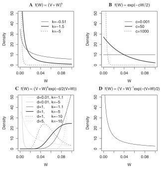
Each of the power, exponential, and hybrid priors are really families of priors because they depend on hyperparameters, whereas the reciprocal prior takes a single density. These hy-perparameters are represented byk,c, andd, and all priors have a support 0<a≤W≤b. We suggest choosing the val-ues ofa,b,c,d, andkvia expert elicitation. Figure 1 shows the densities of some possible priors and hence the range of prior beliefs they can accommodate. We derive the approximate BFs relating to these priors in the supplementary material. All four new BFs can be easily calculated inR[R Core Team, 2012] (code is provided in the supplementary material). It should be noted that what we term the hydrid prior is iden-tical to a shifted inverse gamma distribution on a restricted support.
Eliciting Hyperparameters of the Priors forW
Our new BFs avoid the problem of specifying a fixed value forW, but instead require other hyperparameter specifica-tion for most of the BFs suggested. The hyperparameters would usually be determined through elicitation based on the distribution function of W. The distribution function for
W when using the power prior Bayes factor (PPBF) is given by
F(W)= (V
+W)k+1–(V+a)k+1
(V+b)k+1–(V+a)k+1 a≤W≤b. (4)
So if a single percentile (p1) of the distribution ofWis elicited
(w1) then we findkby equating Equation (4) top1withW
replaced byw1. For the PPBF and exponential prior Bayes
fac-tor (EPBF) this can easily be solved algebraically. The hybrid prior Bayes factor (HPBF) requires some other numerical search method. The distribution functions for all four priors are given in Table 2. A more reliable strategy is to determine suitable hyperparameters by optimizing the fit of multiple percentiles elicited from an expert. For example, if we elicith percentiles (p1,p2, . . . ,ph) ofW(w1,w2, . . . ,wh), then we
find ˆksuch that
ˆ
k=argmink
h
i=1
(V+wi)k+1–(V+a)k+1
(V+b)k+1–(V+a)k+1 –pi 2
. (5)
Rather than directly eliciting Wvalues, it is likely that an expert will find it easier to envisage particular central prob-ability intervals (PIs) for the ORs. For theith percentile to be elicited (pi), let PIu,i represent the upper limit of the
zith central PI for the OR. Then wi can be found using
wi=(ln(PIu,i)/–1(pi))2, wherepi=1–(1–0.01zi)/2. It is
also likely to help if they are encouraged to choose the par-ticular PIsz=(z1,z2, . . . ,zh) themselves.
To calculate ˆk, we also need to specifya,b, andV. Suppose the expert provides the minimum and maximum values of the upper limits of say the 80th percentile (denoted PIu,min
and PIu,max) that they consider plausible. We can use PIu,min
to determineausinga=(ln(PIu,min)/–1(p))2where in this
casez=60,p =0.8 and similarly forbreplacing PIu,minwith
PIu,max. The value ofVwill be different for every SNP, so we
suggest taking the median of the range ofV. The values ofV can be found by fitting univariate logistic regression models to the data whereVis the square of the standard error of the parameter estimate for the SNP. This can be done in many standard statistical software packages.
The values of the hyperparameters in Figure 1 give a good indication of the space over which to search. We have written
Rcode to carry out this search over the hyperparameters. The output includes the minimum sum of squares from Equation (5), so that the form of the prior which results in the smallest value can be determined. This code is available upon request. There are other methods available to determine the hyperpa-rameters, for example, empirical Bayes methods. In empirical Bayes, the hyperparameters () are found as the solution to argmax(p(data|)). In our case, this corresponds to max-imizing the BF over, which cannot be done analytically.
Testing the Properties and Efficacy of the New BFs on Simulated Data
Three of out four forms of BF use the genotype data to inform the prior throughV, the asymptotic variance of the estimate of the logOR.Vwill be different for each SNP since
0.00 0.04 0.08 0 1 02 03 04 05 0 W Density k=−0.51 k=−1.5 k=−5
A f(W)∝(V+W)k
0.00 0.04 0.08
0 1 02 03 04 05 0 W Density c=0.001 c=50 c=1000
B f(W)∝exp(−cW 2)
0.00 0.04 0.08
0 1 02 03 04 05 0 W Density d=0.01, k=−1.1 d=0.01, k=−5 d=1, k=−1.1 d=1, k=−5 d=1, k=−10 d=5, k=−10
C f(W)∝(V+W)kexp(−d/2(V+W))
0.00 0.04 0.08
0 1 02 03 04 05 0 W Density
[image:5.594.133.457.62.403.2]D f(W)∝(V+W)−1exp(−(V+W)/2)
Figure 1. Densities of three families of tractable priors and one specific prior for f(W) (0 <W≤0.1).β1is logOR withβ1∼N(0,W) and a
value ofV = 0.003 is used in all plots.
Table 2. Prior distribution functions forW
Type of prior F(W) Limitations
Power (V+W)
k+1–(V+a)k+1
(V+b)k+1–(V+a)k+1 k< –
1 2,k= –1 ln
V+W V+a /ln
V+b
V+a k= –1
Exponential
exp
–cW
2 –exp
–ca 2 exp –cb
2 –exp
–ca
2
c>0
Hybrid
–k–1, d
2(V+W) –
–k–1, d
2(V+a)
–k–1, d 2(V+b) –
–k–1, d 2(V+a)
d> –β1,k< –1
Reciprocal ln
W+V
a+V +
∞
n=1
(–1)n
nn!
W+V
2
n
–
a+V
2
n
ln
b+V a+V +
∞
n=1
(–1)n
nn!
b+V
2
n
–
a+V
2
n
Distribution functions for each of the four prior forms.
it depends on, among other quantities, the MAF. We used simulated data to generate realistic values ofVand examined their effect on the prior density ofWfor values ofV corre-sponding to SNPs that have an MAF not less than 0.005, as these are the SNPs that we might have sufficient power to
detect with current sample sizes. These datasets were simu-lated usingHAPGEN2 [Spencer et al., 2009] and the European haplotypes of the August 2010 release of the 1,000 genomes data with large sample sizes reflecting those now being gen-erated by disease-specific consortia.
There has been some suggestion that the effect size of causal SNPs may increase with decreasing MAF [Wang et al., 2005]. We investigate whether the three empirical forms of prior implicitly have this property. To assess this we examine how
E(W) changes withV, over a support relevant to studies with sample sizes of 2,000 or more. Since SNPs with lower MAFs have largerV[Slager and Schaid, 2001], an appropriate prior would possess the property that E(W) is a nondecreasing function ofV. Then as the MAF decreases,Vincreases and rarer SNPs have a priori larger effects on average.
We also tested the use of the novels BFs as a method for filtering (narrowing down the set of candidate causal vari-ables) in a fine-mapping study by carrying out such an anal-ysis on simulated datasets with known causal SNPs. We give results for scenarios in which the causal SNP has an MAF of 0.08, for ORs of 1.10, 1.14, and 1.18 and for total sam-ple sizes of 2,000, 4,000, and 20,000 (with an equal number of cases and controls). We simulated 1,000 datasets for this scenario, and illustrate the results using receiver operating
[image:5.594.51.290.472.656.2]characteristic (ROC) curves. Fawcett [2006] outlines several ways to determine ROC curves when they are used to repre-sent a summary of multiple analyses (in this case those on each of the datasets). Our ROC curves present the true and mean false-positive rates (FPRs) over the multiple analyses, but give no indication as to the variation in FPRs between datasets. Fawcett calls the method that we use threshold av-eraging.
Comparing Fine-Mapping Methods for theCASP8Region Using iCOGS Data
The Collaborative Oncological Gene-environment Study (COGS) Consortium have recently carried out a number of studies using a specially developed Illumina array, known as the iCOGS array [Michailidou et al., 2013]. This was designed to fine-map regions that had been previously identified by GWAS, by concentrating a large number of SNPs in regions of interest where there is already thought to be a causal associ-ation with breast, ovarian, or prostate cancer. One such region comprises base positions 201500074–202569992 of chromo-some two, including theCASP8gene. In this region, 585 SNPs were originally genotyped on breast cancer case and con-trol samples from the Breast Cancer Association Consortium and 501 passed quality control checks. A further 1,232 were successfully imputed using IMPUTE2 (Marchini and Howie,
2010), resulting in genotypes for 1,733 SNPs in 46,450 cases and 42,600 controls (total sample size: 89,050). We used both the full dataset and a subset of 5,238 individuals (2,721 cases and 2,517 controls) to assess the impact of our priors on both smaller and larger studies.
Prior to receiving the data, we carried out elicitation with a breast cancer genetics expert who had previously been in-volved in studies into theCASP8region. We then determined the prior distribution that best matched their beliefs and used it to calculate BFs and carry out filtering on the genotype data from iCOGS.
Results
The Dependence of the Prior Densities ofW upon Hyperparameters and the Genotype Data
Figure 1 shows some possible prior densities forW, with V=0.003 for those densities which depend on V. We see that most of the priors put the majority of the weight ofW close to the lower limit of its support (in this case close to zero). Other than being independent of the genotype data, one of the main advantages of the exponential prior over the other forms forf (W) is its ability to provide an almost uniform prior distribution for Wover the range of values likely to be considered appropriate. The HPBF allows for more flexibility in the shape of the prior distribution. In par-ticular, it is the only prior that allows more mass at higher values ofWthan at lower values ofWand the only prior to have a stationary point. While the other priors are mono-tonically decreasing withW, the mode of hybrid prior is at W= –(V+d/2k).
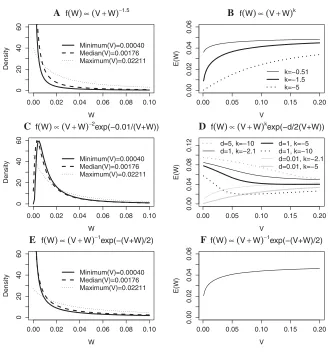
To assess the impact ofVon our priors in an intermediate sized fine-mapping study, we simulated a dataset of size 20,000 (using exactly the same scenario as for the simulated dataset of 4,000) and determined the distribution of values ofVfor those SNPs with MAF≥0.005 and then determined the minimum, median, and maximum of these values to be 0.00040, 0.00176, and 0.02211, respectively. Figure 2 panels (a), (c), and (e) show the prior densities forWfor the power, hybrid, and reciprocal priors for these three values of V, using fixed values of the hyperparameters. While there is some variation in the prior forWasVtakes its maximum and minimum values, for most of the SNPs with MAF ≥0.005 the prior will be relatively similar. There is little reason to suspect these observations will not generalize to other genomic regions.
We next consider SNPs with extreme values ofVas these may lead to extreme priors and potentially large BFs. Because Vis bounded below by 0, we only need to consider extreme large values ofV. If the number of cases and controls is equal and denoted byn, Slager and Schaid [2001] showed thatV∝ 1/napproximately. Studies with total sample sizes of 2,000 will yield most values ofVin the region 0.005≤V≤0.2 for SNPs with MAF greater than 0.005. As sample size decreases occasional large values ofVmay be seen resulting from rare alleles (with MAFs less than 0.005) having very low counts in the case and/or control groups. These SNPs will have broad likelihoods and so are unlikely to have high BFs regardless of the prior. So although very rare alleles may have priors that are different from most of the SNPs, these rare SNPs are unlikely to be retained after filtering.
Are These Priors Consistent with Rare Alleles Having Larger Effects?
There is some suggestion in the literature that rare SNPs might be expected to have larger effect sizes [Wang et al., 2005]. We wanted to assess whether this was the case for our suggested priors. To do this we examined how the ex-pected value of Wvaried withV. If the hypothesis is true then rarer alleles should have larger effect sizes, hence larger values of W. Rarer alleles also have larger values ofV. So if our priors possess this property, we should observe that
E(W) increases withV. For the power, hybrid, and reciprocal priors, the expected value ofWcan either be found directly using integration by parts or by findingE(V+W) by
integra-tion and then using the relaintegra-tionshipE(W)=E(V+W)–V. Those expectations that depend onVare plotted in Figure 2 panels (b), (d), and (f) for values ofVlikely to occur.E(W) is independent ofVfor the exponential prior. For the three expectations which depend onV, we were unable to verify al-gebraically thatdE(W)/dV>0∀V>0, b>a>0 andd, k within the specified limits (where relevant), but Figure 2 plots
E(W) against Vfor a range of values of the hyperparame-ters. Panels (b) and (f) show this appears to be the case for the power and reciprocal prior. However, we can see from panel (d) of Figure 2 thatE(W) could decrease withVfor the hybrid prior. Researchers who believe that rare SNPs will
0.00 0.02 0.04 0.06 0.08 0.10
0
2
04
06
0
W
Density
Minimum(V)=0.00040 Median(V)=0.00176 Maximum(V)=0.02211
A f(W)∝(V+W)−1.5
0.00 0.05 0.10 0.15 0.20
0.00
0.02
0.04
0.06
V
E(W)
k=−0.51 k=−1.5 k=−5
B f(W)∝(V+W)k
0.00 0.02 0.04 0.06 0.08 0.10
0
2
04
06
0
W
Density
Minimum(V)=0.00040 Median(V)=0.00176 Maximum(V)=0.02211
C f(W)∝(V+W)−2exp(−0.01/(V+W))
0.00 0.05 0.10 0.15 0.20
0.00
0.04
0.08
0.12
V
E(W)
d=5, k=−10 d=1, k=−2.1
d=1, k=−5 d=1, k=−10 d=0.01, k=−2.1 d=0.01, k=−5
D f(W)∝(V+W)kexp(−d/2(V+W))
0.00 0.02 0.04 0.06 0.08 0.10
0
2
04
06
0
W
Density
Minimum(V)=0.00040 Median(V)=0.00176 Maximum(V)=0.02211
E f(W)∝(V+W)−1exp(−(V+W)/2)
0.00 0.05 0.10 0.15 0.20
0.00
0.02
0.04
0.06
V
E(W)
[image:7.594.132.462.59.412.2]F f(W)∝(V+W)−1exp(−(V+W)/2)
Figure 2. Prior densities ofW(plots (a), (c), and (e)) andE(W) as a function ofV (plots (b), (d), and (f)) for empirical forms of the prior (0 <W≤0.1). Prior densities are given for minimum, median, and maximum values ofVfor SNPs with MAF> 0.005 in a sample size of 20,000.E(W) is given over a range ofV likely to been seen in sample sizes of 2,000 or greater with different values of the hyperparameters, where relevant.
a priori have larger effects should constraind to be close to zero. Alternatively a generalization of the Savage-Dickey density ratio (Verdinelli and Wasserman, 1995) could be used with a prior of the formWkexp (–d/2W), so removing the
dependence onV. The generalization of the Savage-Dickey density ratio approximates the BF without the need for inte-gration, hence allowing for a wider range of priors. It bases calculation of the BF on a large number of samples from the posterior distributions of the model parameters.
Fine-Mapping Using BFs on Simulated Data
We carried out filtering using WBFs and our new BFs on 1,000 simulated datasets with a single causal SNP with an MAF of 0.08. We chose ORs of 1.10, 1.14, and 1.18 and sample sizes of 2,000, 4,000, and 20,000. We also included the results of filtering usingP-values from univariate logistic regression. Table 3 shows the true-positive rates (TPRs) (×1,000) from the simulated data analysis by sample size, OR, and FPR. We have limited the results to FPRs ≤20% as this more than covers the desired range of FPRs in any fine-mapping procedure. The support for the new priors is 0.003≤W≤
0.1 and so we letW=0.003 andW=0.1 in the WBF in Table 3. In Table 3, we chose hyperparameters for our new priors that place more of the mass at smaller values ofW. The priors for PPBF and HPBF with the specified hyperparameters have similar shaped densities and so, not surprisingly, produce broadly similar rankings.
Table 3 shows that using WBF withW=0.003 yields higher TPRs than using WBF withW=0.1 in many of the scenarios considered. This is perhaps not surprising because the logORs for the causal SNP used in the simulations are all small (0.095– 0.166) and so lower values ofW, which put more weight at small ORs, are expected to perform better. The exception to this is at the lowest FPR whereW=0.1 generally yields higher TPRs. It is at the very low (and arguably most relevant) FPRs that the PPBF and HPBF methods generally outperform all the other methods considered. If we focus on the smallest FPR considered at each level of sample size and OR, we see that either the HPBF or the PPBF have the highest TPR of any of the methods considered in eight out of the nine scenarios. It is only when the sample size is 20,000 and the OR is 1.1 that one of the other methods (WBF withW=0.003) is superior
at the lowest FPR.
Table 3. TPRs (×1,000) from the simulated data analysis by sam-ple size, OR, and FPR
Sample size (SS)
SS=2,000 SS=4,000 SS=20,000 FPR (%) FPR (%) FPR (%) Method
(parameter values) 5% 10% 15% 20% 5% 10% 15% 20% 1% 5% 10% 15% OR=1.10
P-value 72 118 163 259 151 249 320 384 202 497 677 786 WBF (W=0.003) 48 131 216 291 136 285 385 442 231 579 762 836
WBF (W=0.1) 89 126 166 173 152 221 242 259 173 433 530 582 PPBF (k= –1.5) 88 140 202 245 170 264 318 346 224 524 676 758 HPBF (d=0.01, 89 140 204 248 170 263 308 334 225 517 655 707
k= –1.1)
OR=1.14
P-value 146 247 331 395 232 357 457 531 508 831 924 962 WBF (W=0.003) 106 255 376 457 222 408 528 574 502 850 960 979
WBF (W=0.1) 159 248 290 307 239 335 373 387 503 789 875 899 PPBF (k= –1.5) 159 272 331 372 257 386 457 486 536 846 926 956 HPBF (d=0.01, 161 276 332 363 256 387 450 470 539 843 919 943
k= –1.1)
OR=1.18
P-value 178 286 382 454 323 475 551 619 753 950 984 994 WBF (W=0.003) 134 302 430 496 290 500 614 663 730 950 989 997
WBF (W=0.1) 200 298 340 353 328 452 478 495 751 947 980 988 PPBF (k= –1.5) 196 322 397 439 351 496 560 602 767 954 987 994
HPBF (d=0.01, 207 325 396 434 355 493 551 582 770 955 987 994
k= –1.1)
True-positive rates (TPRs) multiplied by a thousand at the most relevant false-positive rates (FPRs) for different filtering methods (PPBF, HPBF, Wakefield Bayes factors, and
P-values) applied to 1,000 simulated datasets with 2,871 SNPs. For PPBF and HPBF, the support is 0.003≤W≤0.1. The data were simulated using the LD structure of theCASP8region for a scenario with a single causal SNP with an MAF of 0.08 for various sample sizes, odds ratios, and FPRs . Figures in bold are those that exceed the TPR obtained usingP-values.
What is somewhat surprising is that even when the sample size is as high as 20,000, there are substantial differences in the performances of theP-value method and the methods using BFs, For example, with a sample size of 20,000, an OR of 1.10 and an FPR of 5%, the TPRs for theP-value and WBF withW=0.003 are 0.497 and 0.579, respectively. The TPR
for the WBF method is nearly 17% bigger than the TPR for theP-value method. Making the same comparison when the FPR is 1% the WBF method is over 14% bigger than the TPR for theP-value (0.231 compared to 0.202).
Figure 3 shows several ROC curves derived from filtering with a causal SNP with an OR of 1.14, an MAF of 0.08 and a sample size of 4,000. Figure 3a shows the whole ROC space while Figure 3b shows the ROC curve for FPRs below 20%. Figure 3 includes the results of filtering using the WBF approximation with W=0.003 and W=0.1 and also the results of filtering using a power prior and a hybrid prior with support 0.003≤W≤0.1. The two new priors were chosen so that the power prior put a lot of mass atW=0.003 and hybrid prior out a lot of mass aroundW=0.1. Consequently,
using the power prior produces an ROC curve similar to that using WBFs withW=0.01 and using the hybrid prior produces an ROC curve similar to WBF withW=0.01. There is clearly a lot of variation in the effectiveness of the WBF filter asWchanges. Putting too much prior weight on large effect sizes clearly leads to poor performance of the WBF when the actual causal effect size is small. The new BFs can be thought of as a weighted average of the BFs over the support ofW and so do not suffer to the same degree as using WBF with a value ofWthat puts a lot of mass at values ofβthat have a low likelihood.
0.0 0.2 0.4 0.6 0.8 1.0
0.0
0
.2
0.4
0.6
0.8
1.0
Mean False Positive Rate
T
rue P
ositiv
e Rate
method and parameters p−value WBF: W=0.003 WBF: W=0.1 PPBF: k=−5 HPBF: d=1, k=−1.1 y=x
0.00 0.05 0.10 0.15 0.20
0.0
0.1
0.2
0.3
0.4
0.5
0.6
Mean False Positive Rate
T
rue P
ositiv
e Rate
method and parameters p−value WBF: W=0.003 WBF: W=0.1 PPBF: k=−5 HPBF: d=1, k=−1.1
[image:8.594.56.544.437.677.2]A B
Figure 3. ROC curves showing the results of WBF, PPBF, HPBF, andP-value filtering. (A) Shows the whole ROC space while (B) shows the ROC curve for false-positive rates below 20%. We useW= 0.003 andW= 0.1 for the WBF analysis. The prior for the PPBF analysis hask= −5 and puts most of the mass close toW= 0.003. The prior for the HPBF analysis hasd= 1 andk= −1.1 and puts most of the weight close toW= 0.1. All filtering was carried out on 1,000 datasets simulated using the LD structure of theCASP8region for a scenario with a single causal SNP that has an OR of 1.14, an MAF of 0.08, and a total sample size of 4,000.
Table 4. Results of analysis of iCOGS data
Ranking WBF with
W=
SNP
number OR (95% CI) MAF PPBF P-value 0.003 0.1 PPBF 980b 1.048 (1.027, 1.071) 0.294 1,387 1 1 1 1
1,027 1.046 (1.024, 1.068) 0.285 664 2 2 2 2 992b 1.045 (1.022, 1.067) 0.287 334 3 3 3 3
909 1.043 (1.021, 1.065) 0.287 234 9 4 6 4 878a 1.081 (1.039, 1.125) 0.061 228 12 13 4 5
1,272a 1.075 (1.036, 1.116) 0.071 217 14 11 5 6
950b 1.043 (1.021, 1.065) 0.286 217 10 5 7 7
838 1.041 (1.020, 1.062) 0.338 213 5 6 10 8 960b 1.043 (1.021, 1.065) 0.285 213 7 =7 =8 =9
961b 1.043 (1.021, 1.065) 0.285 213 8 =7 =8 =9
985b 1.043 (1.021, 1.066) 0.286 206 4 9 11 11
837 1.042 (1.021, 1.064) 0.299 200 6 10 13 12 907 1.042 (1.020, 1.064) 0.287 167 11 12 16 13 896 1.042 (1.020, 1.064) 0.287 166 13 =14 =17 =14 912 1.042 (1.020, 1.064) 0.287 166 15 =14 =17 =14 956a,b 1.052 (1.025, 1.080) 0.170 159 16 16 15 16
681a 1.074 (1.035, 1.116) 0.069 149 17 19 14 17
1,004a,b 1.051 (1.024, 1.078) 0.173 124 18 18 20 18
885 1.041 (1.019 1.063) 0.287 119 19 17 23 19 955a,b 1.050 (1.023, 1.078) 0.173 112 21 21 21 20 a For these SNPs, the major allele is associated with a higher disease risk. b These SNPs were not genotyped but imputed. Top-ranked SNPs inCASP8region
based on power prior Bayes factor (PPBF) approximation with hyperparameter
k= –1.66 anda=0.003≤W≤b=0.1. Rankings usingP-value and Wakefield Bayes factor (WBF) are also included, as is the logistic regression estimate and 95% confidence interval (CI) of the odds ratio (OR) for each SNP. The genotype data forCASP8region come from the iCOGS study and has a total sample size of 89,050 and 1,733 SNPs.
Fine-Mapping Using BFs on the iCOGS Data
Before analyzing the iCOGS data [Michailidou et al., 2013], we carried out elicitation with a breast cancer ge-netics expert. They believed that there was a causal SNP with a small effect size in the CASP8 region on chromo-some two. We initially asked our expert to give an interval of possible ORs at a single percentile. They thought that the 80th percentile of the OR was between 1.05 and 1.3, yield-inga=0.003 and b=0.1. We then asked them to choose three further PIs that they were comfortable thinking in terms of. They provided the 0.95, 0.75, and 0.50 PIs giving (z1, z2, z3)=(95, 75, 50). For these probabilities, we asked
for their best estimate of the upper limit of the OR and the expert provided PIu =(1.43, 1.21, 1.14). From these we get
(w1, w2, w3)=(0.0333,0.0275,0.0377). The median value
ofVfor the SNPs in the iCOGS data was 0.00017. We used all these values to carry out a search over–10≤k< –0.5 at inter-vals of 0.01 for the PPBF. Evaluating Equation (5) for each of these values ofk, we found that for the PPBF, the minimum of the sum of squared differences occurs atk= –1.66. If we use the same method to find other prior forms which fit the elicited values we get an exponential prior withc =145 and a hybrid prior withd=0.001 andk= –1.69. Of these three priors, the power prior has the closest fit to the elicited values and is a better fit than the reciprocal prior, so we used this to calculate the BF for the iCOGS data.
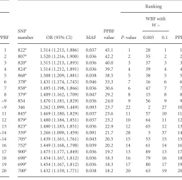
Table 4 contains information about the top 20 ranked SNPs based on the PPBF values calculated from the full iCOGS data.
Table 5. Results of subset analysis of iCOGS data
Ranking WBF with
W=
SNP
number OR (95% CI) MAF PPBF
value P-value 0.003 0.1 PPBF 822a 1.514 (1.215, 1.886) 0.037 45.1 1 28 1 1
807a 1.520 (1.216, 1.900) 0.036 42.2 2 35 2 2
820a 1.515 (1.213, 1.893) 0.036 40.0 3 37 3 3
824a 1.514 (1.212, 1.891) 0.036 39.7 4 39 4 4
868a 1.508 (1.209, 1.881) 0.038 38.5 5 38 5 5
378a 1.431 (1.174, 1.745) 0.046 33.3 7 16 6 6
858a 1.495 (1.198, 1.866) 0.036 30.6 6 47 7 7
379a 1.409 (1.162, 1.709) 0.047 29.2 8 15 8 8
854 1.470 (1.181, 1.829) 0.036 24.0 9 56 9 9 346 1.262 (1.099, 1.449) 0.093 23.7 22 2 27 10 845a 1.469 (1.180, 1.829) 0.037 23.6 11 57 10 11
879a 1.480 (1.184, 1.851) 0.037 23.2 10 64 11 12
823a 1.480 (1.183, 1.851) 0.036 22.9 12 65 12 13
339a 1.266 (1.099, 1.459) 0.091 21.7 28 3 37 14
705a 1.439 (1.161, 1.761) 0.043 20.5 15 53 15 15
752a 1.449 (1.168, 1.798) 0.039 20.2 14 61 14 16
900a 1.475 (1.177, 1.849) 0.036 19.7 13 89 13 17
698a 1.454 (1.167, 1.812) 0.036 18.3 16 79 16 18
699a 1.454 (1.167, 1.812) 0.036 18.3 17 80 17 19
700a 1.432 (1.159, 1.771) 0.038 18.2 20 63 19 20 a These SNPs were imputed.
Ranks of the top-ranked SNPs inCASP8region based on the power prior Bayes factor (PPBF) approximation with hyperparameterk= –1.96 and
a=0.003≤W≤b=0.1. Rankings usingP-value and Wakefield Bayes factor (WBF) are also included, as is the logistic regression estimate and 95% confidence interval (CI) of the odds ratio (OR) for each SNP. Values of the Bayes factors for the PPBF are also provided. The genotype data forCASP8region come from a subset of the iCOGS study and has a total sample size of 5,238 and 1,733 SNPs.
It should be noted that none of these will necessarily be the causal SNP, although previous simulations show us that, with such a large sample size, there is a high probability that the causal SNP will be highly ranked (Spencer et al., 2014). We observe that nine of the top 20 ranked SNPs were among the 501 SNPs genotyped (rather than imputed) in the iCOGS data. Included in the table is the ranking for these SNPs by P-value from univariate logistic regression and by WBF with the two values ofWthat are the extremities of the support used forWwith the PPBF. We can see that while all these methods rank SNPs similarly, with the same SNPs always ranked in the top three, the rankings do differ somewhat.
With such a large sample size, the majority of the informa-tion comes from the likelihood, rather than the prior, which is why the rankings using the different methods are so simi-lar when considering the full iCOGS data. Many association studies will have smaller sample sizes than those used here and in these studies the prior will have more influence on the BFs obtained and so we would expect much more vari-ation in the ranks across the different BFs. We investigated this using a stratified random subset of the iCOGS subjects, with 2,721 cases and 2,517 controls (5,238 total). The same analyses were carried out on this subset of the data and the results are given in Table 5. As expected, the prior has much larger influence in this smaller fine-mapping study. Of the top 20 SNPs selected by PPBF, only four of these are in the top 20 for WBF withW=0.003 (where the prior has most mass around small effect sizes). Of the top 20 SNPs selected
[image:9.594.51.292.72.320.2]by WBF withW=0.003, 10 SNPs are not in the top 50 for PPBF and three are not in the top 75 for PPBF. There is more agreement between WBF withW=0.1 and PPBF but WBF still selects two SNPs in its top 20 that are not in the top 20 for PPBF.
Discussion
Novel BFs and Their Properties
We have developed several new forms of approximate BF. These include three parametric families and one fixed form, each relating to a different prior distribution on W, where we assume that the prior distribution on the logOR of an SNP isN(0,W). This allows for the calculation of BFs where a normal distribution is believed to be an appropriate form for the prior, but where there is uncertainty in W. Most of the priors we suggest forWput most of the weight ofWat the lower end of the support but the exponential prior allows for an almost uniform prior which is useful when an expert believes a range of values ofWare equally likely a priori. The hybrid prior can be specified so that the mode is anywhere in the given range. This might be useful when an expert has a strong prior belief in a particular value ofWbut wants to allow for some uncertainty in it.
Three of these prior forms also depend upon the geno-type data. The expectation ofWappears universally to be an increasing function ofVonly for the power and reciprocal priors. This means that these priors are consistent with the hypothesis that rarer alleles have have larger effects. Depend-ing on the values of the hyperparameters, E(W) may be a decreasing function ofWwhen the hybrid prior is employed. Such a prior would be inappropriate to use if it was believed that rare causal SNPs do indeed have larger effect sizes. In this case, we suggest a Savage-Dickey density ratio approach [Verdinelli and Wasserman, 1995].
All the novel BFs described here are univariate. The solu-tion we have employed in the univariate case relies on recog-nizing the BF integrands as standard probability densities. We did consider extending these BFs to the multivariate case and while specifying the prior in the multivariate case is straight-forward, the resulting integrals appear to be intractable and would probably need to be solved analytically so that easily calculated closed form expressions for the BFs may not be easily available.
Using Novel BFs in Practice
All novel BF approximations can be calculated inR(we give code in supplementary data), although the EPBF is computa-tionally intensive and cannot produce results for SNPs which have very small MLEs of the logOR. The computation for all of the other forms is simple and efficient and we therefore recommend using the PPBF or HPBF instead of the EPBF where possible. In most cases, hyperparameters can be found which result in power or hybrid priors very similar to the de-sired exponential prior. In these situations, we recommend
that the EPBF only be used if the investigator does not want to include any information from the data in the prior.
We described how elicitation may be employed with an expert to determine the most appropriate values for the hy-perparameters, although such experts may find this task dif-ficult. The importance of feedback in the elicitation process is worth emphasizing. Once a distribution forWhas been determined based on the quantiles elicited from the expert, it is important to relay back to them what this means about other quantiles not elicited to check that these are accept-able. A web-based tool, MATCH, which may help with this purpose is now available [Morris et al., 2014].
BF Analysis in Future Genetics
Filtering using BFs has already been used in fine-mapping [Maller et al., 2012] and our more flexible approach is likely to appeal to investigators who struggle to specify a suitable variance for a fixed normal prior. The methods we use as-sume that all SNPs have equal prior odds of being causal, but BFs can also be used to update the odds and then filtering can be carried out using the posterior odds of causality. The effectiveness of BF filtering may be further improved by ap-propriate incorporation of functional information through SNP-specific prior odds. Such functional data can be found on theENCODEdatabase [Encode Project Consortium, 2011],
the RegulomeDB database [Boyle et al., 2012] and the F-SNP database [Lee and Shatkay, 2009]. All functional SNP-level data sources are currently limited as information is not com-plete for all the SNPs across the genome. The FS score found on the F-SNP database has the advantage that it integrates a large amount of data from multiple publicly available data sources. It formally combines scores from a number of bioin-formatics tools using weighting based on the “reliability” of these tools to give a score between 0 and 1. BFs are likely to become increasingly popular as investigators seek to make use of the vast prior functional information available. The new BFs presented in this paper allow researchers more flexibility in the specification of the prior OR, allowing the distribution used to better match expert prior beliefs.
Acknowledgments
We would like to thank the two anonymous reviewers for their helpful comments that helped us to improve the manuscript. This work was carried out as part of a PhD project funded by the Engineering and Physical Sciences Research Council (EPSRC).
We would also like to thank all studies in the Breast Cancer Association Consortium (BCAC) and the Collaborative Oncological Gene-environment Study (COGS) for the use of their data. The COGs study would not have been possible without the contributions of the following: Per Hall (COGS); Paul Pharoah, Manjeet K. Bolla, Qin Wang (BCAC), Andrew Berchuck (OCAC), Rosalind A. Eeles, Douglas F. Easton, Ali Amin Al Olama, Zsofia Kote-Jarai, Sara Benlloch (PRACTICAL), Georgia Chenevix-Trench, Antonis Antoniou, Lesley McGuffog, Fergus Couch and Ken Offit (CIMBA), Joe Dennis, Alison M. Dunning, Andrew Lee, and Ed Dicks, Craig Luccarini and the staff of the Centre for Genetic Epidemiology Laboratory, Javier Benitez, Anna Gonzalez-Neira, and the staff of the CNIO genotyping unit, Jacques Simard and Daniel C. Tessier, Francois Bacot, Daniel Vincent, Sylvie LaBoissire and Frederic Robidoux and the staff of the McGill University and Gnome Qubec
Innovation Centre, Stig E. Bojesen, Sune F. Nielsen, Borge G. Nordestgaard, and the staff of the Copenhagen DNA laboratory, and Julie M. Cunningham, Sharon A. Windebank, Christopher A. Hilker, Jeffrey Meyer and the staff of Mayo Clinic Genotyping Core Facility.
Funding for the iCOGS infrastructure came from: the European Community’s Seventh Framework Programme under grant agreement number 223175 (HEALTH-F2-2009-223175) (COGS), Cancer Research UK (C1287/A10118, C1287/A 10710, C12292/A11174, C1281/A12014, C5047/A8384, C5047/A15007, C5047/A10692), the National Institutes of Health (CA128978) and Post-Cancer GWAS initiative (1U19 CA148537, 1U19 CA148065, and 1U19 CA148112—the GAME-ON initiative), the De-partment of Defence (W81XWH-10-1-0341), the Canadian Institutes of Health Research (CIHR) for the CIHR Team in Familial Risks of Breast Can-cer, Komen Foundation for the Cure, the Breast Cancer Research Foundation, and the Ovarian Cancer Research Fund.
References
Boyle AP, Hong EL, Hariharan M, Cheng Y, Schaub MA, Kasowski M, Karczewski KJ, Park J, Hitz BC, Weng S and others. 2012. Annotation of functional variation in personal genomes using RegulomeDB.Genome Res22(9):1790–1797. Encode Project Consortium. 2011. A user’s guide to the encyclopedia of DNA elements
(ENCODE).PLoS Biol9(4):e1001046.
Fawcett T. 2006. An introduction to ROC analysis.Pattern Recogn Lett27(8):861– 874.
Kass RE, Raftery AE. 1995. Bayes factors.J Am Stat Assoc90(430):773–795. Lee PH, Shatkay H. 2009. An integrative scoring system for ranking SNPs by their
potential deleterious effects.Bioinformatics25(8):1048–1055.
Maller JB, McVean G, Byrnes J, Vukcevic D, Palin K, Su Z, Howson JMM, Auton A, Myers S, Morris A, and others. 2012. Bayesian refinement of association signals for 14 loci in 3 common diseases.Nat Genet44(12):1294–1301.
Marchini J, Howie B. 2010. Genotype imputation for genome-wide association studies.
Nat Rev Genet11(7):499–511.
Marchini J, Howie B, Myers S, McVean G, Donnelly P. 2007. A new multipoint method for genome-wide association studies by imputation of genotypes.Nat Genet39(7):906–913.
Michailidou K, Hall P, Gonzalez-Neira A, Ghoussaini M, Dennis J, Milne RL, Schmidt MK, Chang-Claude J, Bojesen SE, Bolla MK, and others. 2013. Large-scale genotyping identifies 41 new loci associated with breast cancer risk.Nat Genet
45(4):353–361.
Morris DE, Oakley JE, Crowe JA. 2014. A web-based tool for eliciting probability distributions from experts.Environ Modell Softw52:1–4.
R Core Team. 2012.R: A Language and Environment for Statistical Computing.Vienna Austria: R Foundation for Statistical Computing, ISBN 3-900051-07-0. Slager SL, Schaid DJ. 2001. Case-control studies of genetic markers: power and sample
size approximations for Armitage’s test for trend.Hum Hered52(3):149–153. Spencer CC A, Su Z, Donnelly P, Marchini J. 2009. Designing genome-wide association
studies: sample size, power, imputation, and the choice of genotyping chip.PLoS Genet5(5):e1000477.
Spencer AV, Cox A, Walters K. 2014. Comparing the efficacy of SNP filtering methods for identifying a single causal SNP in a known association region.Ann Hum Genet
78: 50–61.
Stephens M, Balding DJ. 2009. Bayesian statistical methods for genetic association studies.Nat Rev Genet10(10):681–690.
Udler MS, Meyer KB, Pooley KA, Karlins E, Struewing JP, Zhang J, Doody DR, MacArthur S, Tyrer J, Pharoah PD, and others. 2009. FGFR2 variants and breast cancer risk: fine-scale mapping using African American studies and analysis of chromatin conformation.Hum Mol Genet18(9):1692–1703.
Verdinelli I, Wasserman L. 1995. Computing Bayes factors using a generalization of the Savage-Dickey density ratio.J Am Stat Assoc90(430):614–618.
Vignal CM, Bansal AT, Balding DJ. 2011. Using penalised logistic regression to fine map HLA variants for rheumatoid arthritis.Ann Hum Genet75: 655–664. Wakefield J. 2008. Reporting and interpretation in genome-wide association studies.
Int J Epidemiol37(3):641–653.
Wakefield J. 2009. Bayes factors for genome-wide association studies: comparison with p-values.Genet Epidemiol33(1):79–86.
Wang WYS, Barratt BJ, Clayton DG, Todd JA. 2005. Genome-wide association studies: theoretical and practical concerns.Nat Rev Genet6(2):109–118.