structure
.
White Rose Research Online URL for this paper:
http://eprints.whiterose.ac.uk/123042/
Version: Accepted Version
Article:
Eltzner, B, Huckemann, S and Mardia, KV orcid.org/0000-0003-0090-6235 (2018) Torus
principal component analysis with applications to RNA structure. Annals of Applied
Statistics, 12 (2). pp. 1332-1359. ISSN 1932-6157
https://doi.org/10.1214/17-AOAS1115
(c) 2018 Institute of Mathematical Statistics. This is an author produced version of a paper
accepted for publication in Annals of Applied Statistics. Uploaded in accordance with the
publisher's self-archiving policy.
[email protected] https://eprints.whiterose.ac.uk/
Reuse
Items deposited in White Rose Research Online are protected by copyright, with all rights reserved unless indicated otherwise. They may be downloaded and/or printed for private study, or other acts as permitted by national copyright laws. The publisher or other rights holders may allow further reproduction and re-use of the full text version. This is indicated by the licence information on the White Rose Research Online record for the item.
Takedown
If you consider content in White Rose Research Online to be in breach of UK law, please notify us by
TORUS PRINCIPAL COMPONENT ANALYSIS WITH APPLICATIONS TO RNA STRUCTURE
By Benjamin Eltzner1,∗, Stephan Huckemann1,∗ and Kanti V. Mardia2,
1Felix-Bernstein-Institute for Mathematical Statistics in the Biosciences,
Georg-August-University G¨ottingen,
2Department of Statistics, University of Oxford and Department of
Statistics, University of Leeds,
There are several cutting edge applications needing PCA methods for data on tori and we propose a novel torus-PCA method that adaptively favors low-dimensional representations while preventing overfitting by a new test, both of which can be generally applied and address shortcomings in two previously proposed PCA methods: Unlike tangent space PCA, our torus-PCA features structure fidelity by honoring the cyclic topology of the data space, and, unlike geodesic PCA, produces non-winding, non-dense descriptors. These features are achieved by deforming tori into spheres with self-gluing and then using a variant of the recently developed principal nested spheres analysis. This PCA analysis involves a step of subsphere fitting and we provide a new test to avoid overfitting. We validate our torus-PCA by application to an RNA benchmark data set. Further, using a larger RNA data set, torus PCA recovers previously found structure, now globally at the one-dimensional representation, which is not accessible via tangent space PCA.
1. Introduction. Dimension reduction on non-Euclidean manifolds with PCA-like methods has been a challenging task for which two usually suc-cessful categories of methods have been developed in the last decades: ex-trinsic (tangent space) approaches, e.g.Gower(1975);Fletcher et al.(2004);
Boisvert et al. (2006); Arsigny et al. (2006), and intrinsic (geodesic) ones, e.g.Huckemann and Ziezold (2006). A critical review of PCA methods has been given inHuckemann, Hotz and Munk(2010);Sommer(2013) is another recently developed intrinsic PCA method. However, for the very simple non-Euclidean case of the flat and compact space of a torus (a direct product space of two or more angles), these approaches are not adequate. Namely,
∗
The authors gratefully acknowledge DFG HU 1575/4, DFG CRC 755 and the Nieder-sachsen Vorab of the Volkswagen Foundation.
Keywords and phrases:Statistics on manifolds, tori deformation, directional statistics, dimension reduction, dihedral angles, fitting small spheres, principal nested spheres anal-ysis
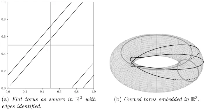
tangent space PCA (TS-PCA) fails to take into account the periodicity of the torus and, even worse, geodesic PCA is completely inapplicable because almost all geodesics densely wind around, as in Figure 1.
(a) Flat torus as square in R2
with edges identified.
(b)Curved torus embedded inR3
.
Fig 1:Flat (1a) and curved (1b) torus representation. Except for horizontal and vertical geodesics (grey) in (1a), and diagonal ones, all other geodesics wind around ((1a) and (1b)). All geodesics (black) with an irrational slope in (1a) are dense.
[image:3.612.129.479.163.351.2]not only geometric but also topological singularities (the tangent space is not homeomorphic to the torus).
At this point we recall that within a sphere of radius r >0, every sub-sphere with the same radiusr is agreat subsphere and one of smaller radius is a proper small subsphere. In this paper we speak of small subspheres to include great and proper small subspheres.
Some torus-specific PCA approaches have been developed apart from TS-PCA and geodesic TS-PCA. Using wrapped normals,Kent and Mardia (2009) circumvent the problem of winding geodesics and provide for an intrinsic parametric model with the same number of degrees of freedom as classical PCA. The PCA used by Altis et al. (2008) is a particular case of Kent and Mardia(2009). Allowing only geodesics that wind around at most once, as proposed by Kent and Mardia (2015), further reduces the degrees of freedom. As discussed in Huckemann and Eltzner(2015) for classical PCA inRnthe space ofk-dimensional affine subspaces (0≤k≤n) has dimension
(n−k)(k+ 1); in contrast for PNS in the n-dimensional sphere, the space of k-dimensional small subspheres has dimension (n−k)(k+ 2) (1 ≤ k ≤ n−1). For this reason (building on PNS), T-PCA more flexibly favors lower dimensional representations than TS-PCA, while this flexibility is better controlled against overfitting than in classical PNS.
Sargsyan, Wright and Lim(2012) may have been the first to treat toroidal data describing RNA structures in a spherical geometry. In their construc-tion, they halved the corresponding seven torus angles defined below and treated them as polar angles from a seven-dimensional sphere, thus tak-ing only a very first step towards T-PCA. On this seven-dimensional sphere they investigated a test data set which we call thebenchmark data. However,
Sargsyan, Wright and Lim(2012) neither discussed nor exploited the dras-tic change of geometry, let alone amended by self-gluing, and only applied geodesic PCA (see Huckemann and Ziezold (2006)), maximizing projected variance and not minimizing residual variance. Incidentally, some pitfalls of using projected variance for compact manifolds were noted in Huckemann, Hotz and Munk(2010).
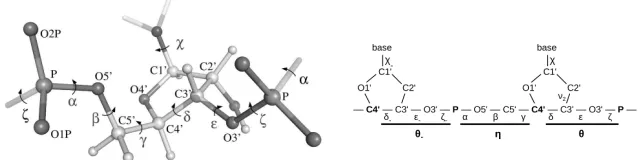
Chen and Varner (2011); Seetin and Mathews (2012); Brewer (2013)). At the bottom level is thesingle residue geometry usually described bydihedral angles between neighboring planes, each spanned by three adjacent atoms, similar to pages of an open book (Figure2). The structure of each nucleotide can be described by 6 angles for the polymeric backbone and one angle for the nucleotide’sbase, giving a total of 7 angles (Figure3 and Table1). Sec-ondary structure is given by self-interaction within the RNA molecule via base pairing and other interactions, forming specific patterns such as A-helices, hairpin loops, and others. At the top level,tertiary and higher order structure arises from interacting lower order structure patterns via further base and backbone bindings.
In contrast to primary structure, the 3D structure is not easily accessi-ble but needs to be reconstructed by elaborate technology such as X-ray crystallography. However, experimental structures are prone to misinter-pretation and various errors. For example, backbone inconsistencies, where different reconstructed atoms occupy the same spatial location, frequently occur during reconstructionRichardson et al.(2008); Jain, Richardson and Richardson(2015). To avoid or correct such errors, the space of possible 3D structures is often restrained or constrained to previously observed struc-tures. This is typically done at the nucleotide or paired nucleotide levelYang et al.(2003); Schneider, Morvek and Berman(2004);Wadley et al. (2007);
ˇ
Cech et al. (2013). Specifically, use is made of so-called rotamers describ-ing empirical modes of probability distributions of nucleotide or nucleotide pair conformations. As these distributions are relatively peaked, limiting the conformational space to such rotamers avoids the introductions of incorrect conformations by limiting the conformational space to previously observed 3D patterns.
Among the many challenges along this path, we discuss two specific ones: data reduction methods and alignment strategies.
conformer groups.
On the one hand, matching RNA strands requires elaborate registration and alignment strategies (e.g. Mardia (2013)), building on statistical (e.g.
Dryden and Mardia (2016); Srivastava and Klassen (2016)) and Bayesian (e.g. Green and Mardia (2006)) shape technology including non-Euclidean averaging and elastic curve representations (e.g.Liu, Srivastava and Zhang
(2011); Laborde et al. (2013)). On the other hand, averaging and explor-ing the 7D sexplor-ingle residue space can be achieved via dynamically simulatexplor-ing similar structures (e.g. Duarte and Pyle (1998); Chen and Garc´ıa (2013);
Estarellas et al.(2015)), and probabilistic approaches to this end require di-mension reduction methods (e.g.Frellsen et al.(2009)). In this context, also for higher order structure prediction, it is necessary to explore not only the variation of single residue geometries typical for specific secondary structure elements but also single residue geometries for intermediate and transition regions between structure elements (e.g.Dunbrack and Karplus(1994);Jain, Richardson and Richardson(2015)).
Applying torus-PCA to RNA structure analysiswe provide for a novel dimension reduction method at residue level and we apply it within the focus of current research to single residue geometries. However, it readily generalizes to simultaneous analysis of geometries of residue sequences (7n angles for n residues) but such an extension is left for future research. We measure effectively the statistical performance of our method by dimension reduction and faithfulness in terms of preserving previously known structure. All of the angles used in our applications are defined in Table 1 and displayed in Figure 3. First we use the benchmark data set of Sargsyan, Wright and Lim (2012) which consists of neighborhoods of three known cluster centers in theη–θ-plot (as in Figure7a, the pseudo-torsion anglesη,
θare depicted in Figure3b, cf. also Table 1). We find that T-PCA retrieves the underlying clusters in an effective way. This benchmark data set is a subset of a large RNA data set carefully selected for high experimental X-ray precision (0.3 nanometers) by Duarte and Pyle(1998), updated byWadley et al. (2007) and analyzed by them and others, for example, Murray et al.
(2003); Richardson et al. (2008). Next we use another subset of this large RNA data set with C2’-endo sugar pucker (this and the other sugar pucker are explained fully in Section3), subsequently called theC2 data set, where we compare our method to TS-PCA and show that T-PCA captures not only much more variance in the one-dimensional subspace, also the wrong topology in TS-PCA hides and tears apart subtle structural similarities.
1D T-PCA representation, generalizing the above finding of Murray et al.
(2003) that RNA backbone is locally rotameric at heminucleotide level, to:
These RNA conformers are rotameric at full residue level, possibly in a non-linear sense, however.
Fig 2:Illustration of a dihedral (torsion) angle defined by four atoms or three bonds, it is the opening angle between two pages of a book. (Reproduced from
Mardia(2013).)
(a)3D structure of an RNA residue. (b)2D scheme of an RNA residue.
Fig 3: Part of an RNA backbone (Phosphate groups with central atom de-noted by P, followed by sugar rings that connect along the atoms labeled by C4’ and C3’, to which a nucleic base is bound). Dihedral angles (Greek letters) are defined by three bonds, the central bond carries the label; pseudo-torsion angles (bold Greek letters) are defined by the pseudo-bonds between bold printed atoms (Figure 3b). Underlying each pseudo torsion angle are three heminucleotide angles. The precise definitions with same canonical atom notation are given in Table 1. The subscript “−” denotes angles of the neighboring residue. Figure3ais reproduced from Frellsen et al. (2009).
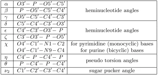
[image:7.612.146.461.196.290.2] [image:7.612.141.462.371.451.2]Table 1
Atom bonds (2nd column) defining angles (1st column) with description (3rd column). The two sets of heminucleotide angles (each of which can be approximated by a pseudo torsion angle) define the backbone, which in conjunction with the base angleχdefine a
residue. Figure3ashows the geometry of these atoms. (N denotes nitrogen.)
α O3′− P −O5′−C5′
heminucleotide angles β P −O5′−C5′−C4′
γ O5′
−C5′−C4′−C3′
δ C5′
−C4′−C3′−O3′
heminucleotide angles ǫ C4′
−C3′−O3′−P
ζ C3′
−O3′−P −O5′
χ O4′
−C1′−N1−C2 for pyrimidine (monocyclic) bases
O4′
−C1′−N9−C4 for purine (bicyclic) bases
η C4′
− P −C4′−P pseudo torsion angles
θ P −C4′−P −C4′
ν2 C1 ′
−C2′−C3′−C4′ sugar pucker angle
and further illustrations in Supplement A. An implementation of our T-PCA method and the RNA data sets we use are included as supplementary materialSupplement B,Supplement C and can be found under
http://www.stochastik.math.uni-goettingen.de/SFB755 B8.
Residues and residual variance. To avoid confusion, we clarify that the biochemical termresidue denotes a RNA molecule segment correspond-ing to a scorrespond-ingle nucleic base (Section3) whereas the statistical termresidual variance denotes unexplained variation (Section 2.3).
2. Torus PCA. Our dimension reduction procedure proceeds in two steps. First, the data space is deformed from a torus to a sphere with self-gluing, i.e. parts of the sphere are topologically identified with themselves, see Figures 4 and 5. Several degrees of freedom are present in the defor-mation map we propose and we discuss consequences of specific parameter choices. The second step is the dimension reduction for which we use a well established procedure for dimension reduction on spheres with some exten-sions to take into account the original torus geometry and the self-gluing of the sphere.
2.1. Torus Deformation Schemes. LetTD = (S1)×D be theD-dimensional
unit torus and SD = {x ∈ RD+1 : kxk = 1} the D-dimensional unit
sphere, D ∈ N. The definition of the data-adaptive deformation mapping
P :TD −→ SD defined in this section is based on comparing squared
is given by the squared Euclidean line element
ds2TD = D
X
k=1
dψk2.
For SD, in polar coordinates φk ∈ [0, π] for k = 1, . . . , D−1 and φD ∈ [0,2π]/ ∼, whose relation to embedding Euclidean coordinates xk is given
by
x1 = cosφ1
∀2≤k≤D : xk=
k−1
Y
j=1
sinαj
cosφk
xD+1 =
D Y j=1 sinφj ,
the spherical squared line element is given by
ds2SD =dφ21+ D
X
k=2
k−1
Y
j=1
sin2φj
dφ2k.
(1)
In fact, this squared line element is not defined for the full sphere but only for φk ∈ (0, π) (k = 1, . . . , D−1), i.e. the singularities of φk = 0, π are
excluded. The singularities at φk = 0, π will account for singularities of P
which results in a self-gluing as explained below.
Angular distortions in a spherical geometry. Following colloquial usage, we use “distortion” synonymous with “deformation” in the following. Because in (1), dφ21 comes with the factor 1, no deformation at all occurs forφ1, i.e. this angle corresponds to spherical distances without distortion.
In the summation for k = 2, we have a factor sin2φ1 of dφ22, which shows
how the angle φ1 distorts the angle φ2 and finally the deformation factor
QD−1
j=1 sin2φj of dφ2D reflects the distortions of φD by all other angles. For
this reason, in the following, we will refer toφD as theinnermost angle and
toφ1 as theoutermost angle.
We now make an important note for later use.
Remark 2.1. Near the equatorial great circle given by φk = π2 (k =
1, . . . , D−1) the squared line element ds2 is nearly Euclidean. Distortions
are higher when anglesφk with low values of the indexk (outer angles) are
close to zero orπ, than when anglesφkwith high values of the indexk(inner
angles) are close to zero or π.
Definition2.2 (Torus to Sphere Deformation). With a data-driven per-mutation p of {1, . . . , D}, data-driven central angles µk (k= 1, . . . , D) and
data-driven scalings αk, all of which are described below, set
φk= π
2 +αp(k)(ψp(k)−µp(k)), k= 1, . . . , D (2)
where p(k) is the index kpermuted by pand the difference (ψp(k)−µp(k)) is
taken modulo2π such that it is in the range (−π, π].
We now explain in detail how the choices are data-driven. Further illustra-tion including practical advice is given in Supplement A. First, we comment on the general applicability of T-PCA.
Remark 2.3. The singularity set introduced, forms a subtorus of di-mension D−2. In consequence, T-PCA is applicable, whenever there is a structural data gap in all angles except for at most two; the larger the gap, the higher the structural fidelity.
In general, the scalings are restricted to the choices αk′ = 1/2 and
αk′ = 1, k′ =p(k). If all of the k′-th torus angles of the data are within an
interval of lengthπ, choose αk′ = 1 (k′ = 1, . . . , D−1) leading to unscaled
(U) angles. Otherwise, we choose αk′ = 1/2 (k′ = 1, . . . , D−1) leading to
halved (H) angles. In practical situations, the torus data are often spread out over more than half circles for several angles. Then we choose (H) angles. In fact, for all of the analyses below, we chose (H) angles and discuss below only the gluing effects corresponding to (H) angles. Notably, the innermost angle φD always remains unscaled: αD = 1. This is depicted in the second
row of Figure5.
The central anglesµk will be chosen such that the mapped data points
come to lie near the equatorial great circle and omit the singularities. Two plausible choices are:
(i) with the circular intrinsic meanψk,intr, setµk=ψk,intr to obtainmean
centered data;
(ii) withψk,gap, the center of the largest gap between neighboringψkvalues
of data points and ψ∗
k,gap its antipodal point, define µk = ψk,∗gap to
While the implementation for (ii) is straightforward, for (i) we have used the fast algorithm from Hotz and Huckemann (2014). Mean-centered data has the merit that the intrinsic means for each angleφk are mapped to the equatorial great circle thus minimizing deformation of the data.
For a strongly skewed data distribution, say, spread out over a half circle, mean centered data using halved angles may touch the singularities, leading to high distortion there, while gap centered data will still be confined to a π/2 neighborhood of the equator. On the other hand, for data sets with outliers, gap centered centering may be less robust than mean centered, making the latter more favorable, as depicted in Figures5c and 5e.
Remark 2.4. Robustness w.r.t. outliers is surprisingly different on a compact space than on the usually considered non-compact spaces. Specific loci of outliers occurring nearly antipodal to the data bulk do not much af-fect the location of the mean, the largest data gap, however, is much more sensitive to these loci.
The choice of the permutation pk is driven by analyses of the data spread
σk2=
n
X
i=1
(ψk,i−µk)2, k= 1, . . . , D
(3)
for each angle, whereψk,i∈S1are the torus data andnis the number of data
points onTD. If the angles are ordered by increasing data spread, such that σp2(1) is minimal andσp2(D)is maximal, in view of Remark 2.1, the change of distances between data points caused by the deformation factors sin2φj in Equation (1) is minimized. We call this orderingspread inside (SI), because variation is concentrated on the inner angles of the sphere. The opposite ordering is called spread outside (SO). Figure 5 illustrates different effects of SI and SO ordering of angles. We will restrict our considerations to these two options.
Self-gluing in case of halved angles: “From a donut to a sausage”.
In the following, we give a brief overview of this procedure for (H) halved-angles (not for (U) halved-angles for the reasons given above).
Due to periodicity on the torus, ψk = 0 is identified with ψk = 2π for all k = 1, . . . , D. In contrast, for all angles φk (k = 1, . . . , D−1), φk =
0 denotes spherical locations different from φk = π. For a representation
φ1, . . . , φD−1 which are set to fixed values in {0, π}. In the topology of the
torus, all those regions with a specific choice of fixed angles are identified with one-another. In particular, there are 2(D−1) such regions of highest dimension D−2 on the sphere (where only one angle is fixed to 0 or π), two of which are pairwise identified in the topology of the torus. In fact, in the topology of the torus, each of theseD−1 regions of highest dimension
D−2 itself carries the topology of a torus of dimension D−2, each glued to each other torus along a subtorus of dimension D−3, and so on. Thus theself-gluing of SD giving the topology ofTD can be iteratively achieved
along a topological subsphere of dimensionD−2 which is suitably divided into 2(D−1) regions that are pairwise identified by way of a torus, sharing common boundaries which correspond to lower dimensional tori.
Example 2.5 details the case D = 3 and Figures 4 and 5 illustrate the caseD= 2 as well as different choices for the permutation p.
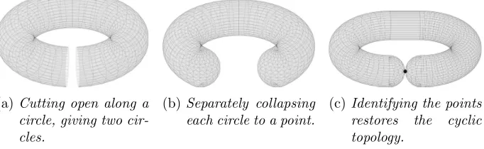
(a)Cutting open along a circle, giving two cir-cles.
(b)Separately collapsing each circle to a point.
(c)Identifying the points restores the cyclic topology.
Fig 4: Self-gluing of T2: From a donut to a sausage. These operations are
only topological, Figure 5 reflects the changes in geometry.
Example 2.5. For D= 3, onS3 we have the squared line element
ds2=dφ21+ sin2φ1 dφ22+ sin2φ2dφ23
,
where the angle ranges areφ1, φ2 ∈[0, π], φ3 ∈[0,2π).
Due to the spherical geometry in the region determined byφ1 = 0 modπ
orφ2 = 0 mod π, the circle φ3 ∈[0,2π) is a single point, say, φ3 = 0. This
region is a topological circle on S3 comprising four arcs
A1 ={(0, φ2,0) : 0≤φ2< π}, A2 ={(π, φ2,0) : 0≤φ2 < π},
A3 ={(φ1,0,0) : 0≤φ1< π}, A4 ={(φ1, π,0) : 0≤φ1 < π}.
Imposing the topology of the torus, when using halved angles, forφ1 and
[image:12.612.137.478.321.426.2]A1 withA2 and of A3 withA4 with endpoints identified as one single point,
forming a topological figure eight.
2.2. Linking the Torus’ Deformation to PNS. For data sets on a torus, having applied a deformation on the resulting self-gluedSD (see Section2.1), we modify principal nested sphere analysis (PNS) by Jung et al. (2010);
Jung, Dryden and Marron(2012) for dimension reduction.
Assume a d-dimensional sphere Sd ⊂ RD+1 with center x ∈ RD+1 and
radius r > 0, and an affine d-dimensional plane Ad ⊂RD+1 with distance
s < r from x. For d≥2 then the intersection Sd∩Ad⊂RD+1 is a (d−
1)-dimensional subsphere Sd−1 of Sd with radius r = √1−s2. If r = 1 (i.e.
s = 0) this subsphere is a great subsphere, otherwise it is a proper small subsphere. Ford= 1 we pick just one pointµ, writing in expedient abuse of notation:S0 ={µ}. In order to include all, great, proper small subspheres and the ultimate point, we call thesesmall subspheres.
The PNS iteration leads to a sequence of small subspheres
SD ⊃SD−1 ⊃ · · · ⊃S2 ⊃S1 ⊃S0={µ}, (4)
where the ultimate pointµis called thenested mean. EachSd(d= 1, . . . , D)
is a d-dimensional sphere, the radii of which decrease monotonically with decreasing dimension (due to nesting). At each reduction step, the residual variances not explained by the corresponding subsphere are given as signed distances: points lying inside the small subsphere – if it is a proper small sphere – receive a positive distance, points lying outside a negative distance. Indeed, for most realistic data applications, with probability one, all sub-spheres are proper small subsub-spheres. However, to avoid overfitting, we want to ensure that the “small subsphere” is not too small but rather a great sub-sphere is fitted; see Section2.4. In this case the direction of positive distance is picked at random. Similarly, we pick the direction of positive distance at random for the reduction fromd= 1 to d= 0.
The classical PNS algorithm consists of two parts which alternate, namely the fitting of a subsphere Sd and the projection to this subsphere πd :
Sd+1 → Sd (d = D−1, . . . ,0) giving the fitted values explained by this
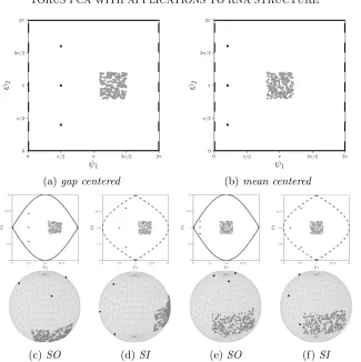
(a)gap centered (b)mean centered
(c)SO (d)SI (e)SO (f) SI
Fig 5:All possibilities for gluing for T2, illustrated by a data set uniform in a square with three outliers. Using mean centered (5b), the square is near the equatorial great circle (ψ1 = π for SO (5e) and ψ2 = π for SI (5f))
and thus the square suffers little distortion, in comparison to the outliers. For gap centered (5a), the outliers are less distorted and for SO (5c) the square is particularly distorted because the equatorial great circle (ψ1 =π)
is then between outliers and square. In both cases, SO decreases the spread of the outliers, SI increases it, more drastically for mean centered. Due to the torus’ periodicity, lines of same type in the flat torus angle plots (top row,
[image:14.612.148.473.97.423.2]For the second step, we use the torus metric
δ:TD×TD →R≥0 (p, q)7→
D
X
i=1
min |pi−qi|2,(2π− |pi−qi|)2 !
1 2
.
Assuming a data set A and a corresponding adaptive deformation PA :
TD →SD we define the following function on the sphere
˜
δ:SD×SD →R≥0 (x, y)7→δ P−1
A (x), P −1 A (y)
(5)
using the inverse deformationPA−1, which is well-defined except for the sin-gularities which are of dimensionD−2. This is a metric when we take into account the topological identifications. To considerably lower computational speed for data analyses, we orthogonally project data to lower dimensional subspheres using the spherical geometry only. On the deformed torus this can be viewed as a non-orthogonal projection. For the minimization in the second step, however, we use ˜δ as the distance function.
2.3. Comparing Variances. In Euclidean spaces, PCA variances are ad-ditive with monotone decrements leading to a convex variance plot as a prop-erty of the metric because decrements correspond to the non-increasingly or-dered eigenvalues of the corresponding covariance matrix. This means that every component can be thought of as contributing a fixed amount of vari-ance and thus the sum of such individual varivari-ances can be understood as ex-plained variance. If one views the principal components as defining a nested sequence of subspaces, the amount of variance which is not explained by the components spanning the subspace is equal to theresidual variance of data around the subspace. Explained variance and residual variance add to 1 and thus yield equivalent descriptions of data variance.
In non-Euclidean spaces, linear PCA is not applicable and non-linear di-mension reduction methods do not come with a similar notion of additive variance (see the discussion for various definitions of intrinsic variances in
Huckemann, Hotz and Munk (2010)). This means that explained variance can no longer be defined in a straightforward way. However, residual vari-ance is still a well-defined notion, therefore we use residual varivari-ances in the following to define cumulative variances, and to compare results of different approaches.
Recall that T-PCA just as PNS yields a sequence of subspaces SD ⊃
SD−1 ⊃ · · · ⊃ S1 ⊃ S0 = {µ} with projections π
d : Sd+1 → Sd ⊂ Sd+1
(d= 0, . . . , D−1). From these we define the iterated projections
and finally theresidual variances (variance not explained by Sd) of a data
setA
VA,PA,d =
X
q∈A
˜
δ2(q,Πd(q)), d= 0, . . . , D−1
and VA,PA,D = 0, where ˜δ is from (5). Due to nestedness, these sequences
are non-increasing with d. However, the decrements VA,PA,d−1 −VA,PA,d
(d = 1, . . . , D) are not necessarily non-increasing, so the resulting curve
in the variance plot need not be convex. Still, this allows to define that {µ}, S1, . . . , Sdexplain thecumulative variance up to dimensiond
VA,PA,0−VA,PA,d, d= 0, . . . , D
which is non-decreasing ind.
2.4. Avoiding Overfitting. In the PNS algorithm a cluster of points con-centrated around a single center may still be best fitted by a “very” small subsphere. As this overfitting is obviously undesirable, Jung, Foskey and Marron (2011); Jung, Dryden and Marron (2012) have fitted a great sub-sphere in such cases:Jung, Foskey and Marron(2011) have given a decision rule whereas Jung, Dryden and Marron (2012) have given a test for this purpose. We propose the following new test based on a geometrically better suited model and highlight its attractive properties, in particular we show how robust is our test under the null model of Jung, Dryden and Marron
(2012), that is a misspecified model for our case. We also indicate some limitations of the two previous procedures.
New model. Let Sd be a fitted small subsphere, 2 ≤d < D. For ease
of notation, we now move and rescale Sd to the unit sphere Sd, without
loss of generality, andp ∈Sd is the center of the, also moved and rescaled, fitted small subsphere Sd−1 ⊂ Sd. For our purpose, we can restrict our
probability model for q ∈ Sd, say, g(q;p), to depend only on the angular
distance r=d(p, q)∈[0, π]. Further suppose that volSd denotes the surface
volume of the d-dimensional unit sphere. Then, due to symmetry, g fully characterizes thespherical angular marginal density of r
h(r;p) := volSd−1 ·g(γ(r);p), r ∈[0, π].
(6)
Here, γ is any curve along a great circle connecting p with its antipodal, parametrized byr ∈[0, π] such that∀r : d(p, γ(r)) =r. Using the spherical volume element dSdΩ(q) at q=γ(r) we note that
1 =
Z
g(q;p)dSdΩ(q) =
Z
h(r;p) volSd−1
dSdΩ(q) = π
Z
0
which means that h(·;p) is indeed a marginal density with respect to the spherical angular measure
dµ(r) = sind−1(r)dr, r∈[0, π].
Then the Lebesgue angular marginal density f(·;p) ofr is defined as
f(r;p) := sind−1(r)h(r;p), π
Z
0
f(r;p)dr= 1,
since it gives the marginal density corresponding to h(·;p) with respect to the Lebesgue measure on [0, π].
Note that these densities are well studied for d= 2 where the angle r is called colatitude (see for example, Mardia and Jupp (2000)); the uniform distribution in polar coordinates for anydon which this discussion is based, see, for example,Mardia, Kent and Bibby (1979).
For the following, we will need the density of the “folded normal distri-bution” on [0,∞):
F(r;ρ, σ) :=√1 2πσ
exp
−(r−ρσ) 2
2σ2
+ exp
−(r+ρσ) 2
2σ2
.
That is, we have
F(r;ρ, σ) =√2 2πσ exp
− r 2
2σ2 −
ρ2
2
coshrρ
σ
, r≥0.
(7)
This density has two positive parameters, ρ and σ. Note that here r is on [0,∞) so it is not restricted to [0, π], a fact which will be of importance later on where we will truncate this distribution. Forρ→ ∞this tends to a usual normal distribution centered atρσ, while it becomes a halved normal distribution (of doubled height) for ρ →0. For ρ ≤1 the mode stays fixed at the origin, forρ >1 it moves to the right.
With the above discussion on the marginals we therefore choose g ∝ F
yielding the spherical angular marginal densityhand the Lebesgue angular marginal densityf:
h(r;p, ρ, σ) := √
2πσ
C(ρ, σ)F(r;ρ, σ), (8)
f(r;p, ρ, σ) := √
2πσ
C(ρ, σ)sin
d−1(r)
where we have truncated F(r;ρ, σ) from (7) and C(ρ, σ) is the normaliza-tion. These will be referred to ash- and f-distribution, respectively, in the following.
Subsequently, it will be important to note the following property of these distributions, for dimensiond= 2, as a surface of revolution overR2. In polar coordinates (r, ϑ)7→ F(r;ρ, σ)21π, the caseρ >1 yields a ring while the case
ρ= 0 yields a symmetric Gaussian distribution. Due to its smoothness it is a good candidate for a test distribution for the angular spherical marginal density (6) to distinguish “just” concentrated data near p (p is at r = 0) from concentrated data along a distinct subsphere (a ring in 2D) aroundp.
Likelihood ratio test. Suppose we are given the sample {q1, . . . , , qn}
from the f-distribution with the spherical distances ri = d(p, qi) (i =
1, . . . , n) where the center p of the subsphere is known. If ρ ≤ 1, the h
distribution has its maximum atr= 0, i.e. there is no proper small spheri-cal structure about the center p. If ρ >1, there is a proper small spherical structure about the centerp. Thus,ρ= 1 forms the boundary between the two cases.
Therefore, we can formulate our hypotheses as follows for testing for a great subsphere.
H0 :ρ= 1 (great subsphere) vs.H1 :ρ > 1 (small subsphere).
(9)
The log likelihood up to a constant is given by
ℓ(ρ, σ|{ri}ni=1) =−nlnC(ρ, σ) + (d−1)
n
X
i=1
ln sin(ri)
−nρ 2
2 −nln(σ) +
n
X
i=1
− r 2
i
2σ2 + ln cosh
riρ
σ
.
Note that the normalizationC(ρ, σ) can be easily computed numerically so we can determine the MLEs forρ andσusing standard numerical optimiza-tion. ForH1, the MLEs need to be constrained underρ >1. Then twice the
log of the likelihood ratio (with negative sign) is given by
λ=2 sup{ℓ(ρ, σ|{ri}ni=1) :ρ∈(1,∞), σ∈R+}
(10)
−2 sup{ℓ(ρ, σ|{ri}in=1) :ρ= 1, σ ∈R+}.
From Wilks’ theorem, the statisticλ, underH0, is asymptotically distributed
asχ21. We use a 5% significance level for our test, which means that when
H0 is rejected, we keep the fitted small subsphere if λ > χ21,0.95 ≈ 3.84;
Comparison with the decision rule ofJung, Foskey and Marron (2011).This rule is based on another type of angular h and f (versus our angularf and h given by (8))
hJ ung(r;p, ρ, σ) :=
1
sind−1(r)F(r;ρ, σ), fJ ung(r;p, ρ, σ) :=F(r;ρ, σ).
In their decision rule, a great sphere is fitted if the probability distribution does not exhibit a ring-shaped local maximum, which is the case if ρ ≤ 2. But this model leads to a singularity of the density hJ ung at p, which is not a desirable feature. In contrast, our h-distribution leads to a smooth distribution on the sphere as illustrated by the above considerations about the surface of revolution. Our h distribution is compared with the hJ ung
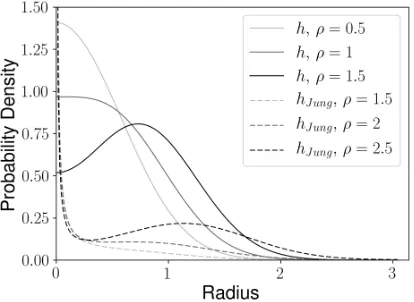
distribution in Figure 6 for appropriate values of ρ. Our h distribution is the same for all dbut for illustration, we have used d= 2 for hJ ung which depends ond.
Fig 6:The probability densities for σ= 0.5 along the geodesic γ in Sd from (6) for our h (invariant under d) and the hJ ung (for d = 2) distribution. Displaying a value forρ below the respective boundary, at the boundary and above the boundary; namely, ρ = 1 for our h and ρ = 2 for the hJ ung
distribution.
In validation of our testwe carried out two simulation studies.
D0: We simulate data underH0 in (9) by choosingρ= 1 in (8) and average
[image:19.612.202.409.339.490.2]D1: We simulate data under H1 in (9) by choosing various combinations
[image:20.612.131.481.224.309.2]of ρ ∈ {1.2,1.5,2,3} and σ ∈ {0.15,0.2,0.5} in (8), and for each we average using 1000 samples.
Table 2
Type 1 errors (rejectingH0) forD0 and Type 2 errors (acceptingH0) forD1 for our test with various parameter values in a simulation with1000repetitions and asymptotic level
of5%, i.e. rejecting forλ > χ2
1,0.95≈3.84withλfrom (10). Type 1 (D0) Type 2 (D1)
Sample size ρ= 1 ρ= 1.2 ρ= 1.5 ρ= 2 ρ= 2 ρ= 3 σ= 0.15 σ= 0.2 σ= 0.2 σ= 0.5 σ= 0.15 100 7.4% 80.4% 41.2% 3.4% <0.1% <0.1% 200 5.5% 73.2% 20.2% <0.1% <0.1% <0.1% 500 5.0% 59.7% 1.0% <0.1% <0.1% <0.1% 1000 4.9% 34.7% <0.1% <0.1% <0.1% <0.1%
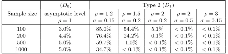
Table 3
We estimate the asymptotic level for our test leading to a true level of5% i.e. achieving a Type 1 error (rejectingH0) forD0 of5%. The table gives the asymptotic level and
Type 2 errors (acceptingH0) forD1 for our test with various parameter values in a simulation with1000repetitions.
(D0) Type 2 (D1)
Sample size asymptotic level ρ= 1.2 ρ= 1.5 ρ= 2 ρ= 2 ρ= 3 ρ= 1 σ= 0.15 σ= 0.2 σ= 0.2 σ= 0.5 σ= 0.15 100 3.0% 85.0% 54.4% 5.1% <0.1% <0.1% 200 4.4% 76.4% 24.2% 0.1% <0.1% <0.1% 500 5.0% 59.7% 1.0% <0.1% <0.1% <0.1% 1000 5.0% 34.7% <0.1% <0.1% <0.1% <0.1%
The results in Table 2 show that our test at asymptotic level of 5%, i.e. it rejects a small sphere when λ > χ21,0.95 ≈ 3.84 with λ from (10), holds asymptotically the level and that the Type 2 error asymptotically decays to zero, very quickly for larger ρ. Since for N = 100,200 the true levels are above 5%, we have estimated the asymptotic levels yielding a true level of 5% in Table 3 and display the corresponding Type 2 error there also. This estimation is a matter of minutes forN = 100 and below one hour for
[image:20.612.124.487.402.489.2]we have used our test against overfitting a small sphere at asymptotic level of 5%.
Assessment of robustness of our test under the null distribution of Jung, Dryden and Marron (2012).We now assess the robustness of our test under a misspecified model, namely, the von Mises-Fisher distribu-tion which is the null distribudistribu-tion of Jung, Dryden and Marron(2012). To carry this out, we note the following points related to their test. First, we note that they have translated their null hypothesis of a compact cluster into fitting by a great subsphere through a von Mises-Fisher distribution. The parameters of this distribution are estimated via MLE. Then a Stu-dentt-like test statistic of distances to the estimated center point is used as their test statistic. Next, we note that for their test statistic, they simulate bootstrap quantiles from the von Mises-Fisher distribution with parameters given by the MLE. However, Jung, Dryden and Marron (2012) have given neither a theoretical result – like we have the asymptotic p-value of our test statisticsλ– nor a simulation study to assess their test statistics under their null hypothesis. We have reimplemented their data driven procedure so as to use their null hypothesis and have carried out the following simulation study.
D0′: Here, we directly simulate spherical samples leading to a great cir-cle, from the null hypothesis of the test of Jung, Dryden and Marron
(2012), namely from a von Mises-Fisher distribution with density inx
proportional toeκµTx
with a high value of the concentration parame-terκ= 10 to give a fair chance. We average over 1000 samples withµ
[image:21.612.179.431.549.606.2]uniform on the sphere.
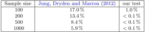
Table 4
Type 1 errors (rejecting the null hypothesis ofJung, Dryden and Marron(2012) which is a von Mises-Fisher distribution) for the test ofJung, Dryden and Marron(2012) and errors under this misspecified model for our test, with concentration parameterκ= 10 in
a simulation with1000repetitions. For their test we use a simulated level of5%and for our test we use an asymptotic level of5%.
Sample size Jung, Dryden and Marron(2012) our test
100 17.0 % 1.0 %
200 13.4 % <0.1 %
500 8.4 % <0.1 %
1000 5.9 % <0.1 %
sample size, and almost reaches the simulated level forN = 1000. In passing, we note that estimating the simulated level leading to a true level of 5% for the test byJung, Dryden and Marron(2012), however, is impractical, as for
N = 100 already, estimation takes weeks.
3. Application to RNA Structure. RNA is usually single-stranded and the single strand interacts with itself, forming complex shapes (this is in contrast to DNA which usually takes a double-stranded helical confor-mation). This means that the geometry is rather variable even on the scale of single atoms. As described in Section 1, each nucleic base corresponds to a backbone segment described by 6 dihedral angles and one angle for the base, giving a total of 7 angles, cf. Table1 and Figure 3. The distribu-tion of these 7 angles over large samples of RNA strands have been studied in detail, see Murray et al. (2003); Schneider, Morvek and Berman (2004);
Wadley et al.(2007);Richardson et al.(2008);Frellsen et al.(2009). Figure
3adetails a segment of the RNA backbone with seven angles for each residue giving the 3D folding structure. An approximation of the geometric folding structure on the level of single residues is given by the two pseudo-torsion angles η and θ (Figure 3b). These two (dihedral) angles provide at once a two-dimensional visualization (Figure7a), see e.g. Duarte and Pyle (1998);
Wadley et al.(2007).
Finally, the dihedral angleν2 (Figure3band Table1) quantifies the
fold-ing (pucker) of the sugar rfold-ing. Only two modes of foldfold-ing are geometrically and energetically possible, which are characterized by either C3’ or C2’ be-ing outside the plane spanned by C1’-O1’-C4’ and towards the direction of O5’. If C2’ lies outside the plane then ν2 ≈ 325◦, this is called C2’-endo
sugar pucker, whereas if C3’ lies outside the plane then ν2 ≈ 35◦, this is
calledC3’-endo sugar pucker. The hydroxy group attached to the C2’ atom in RNA causes the C3’-endo sugar pucker to be energetically preferred (see e.g. Egli, Portmann and Usman (1996)) and thus this is about 10 times more abundant than the C2’-endo sugar pucker in the large RNA data set ofDuarte and Pyle(1998) andWadley et al. (2007).
For our application below we use two subsets of a large classical data set (8301 residues) which was carefully selected for high experimental X-ray precision (0.3 nanometers) by Duarte and Pyle(1998), updated byWadley et al. (2007) and analyzed by them and others, for example, Murray et al.
(2003);Richardson et al.(2008).
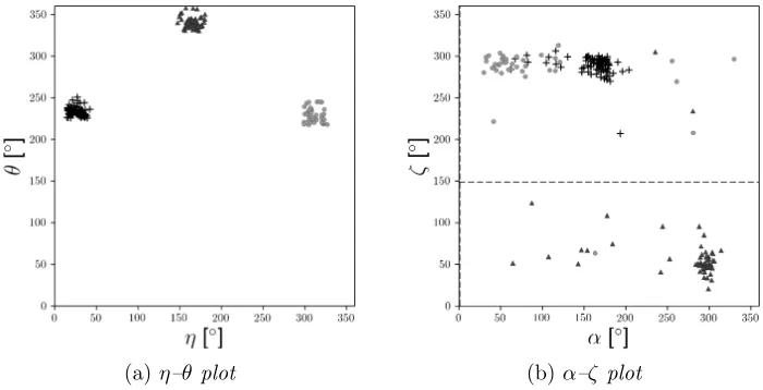
59 points), II (“crosses”, 83 points) and V (“disks”, 39 points) byWadley et al.(2007) totaling 181 data points, which form three clusters in the η–θ
plot as shown in Figure 7a. While clusters I and II correspond to distinct structural elements featuring base stacking, the residues in cluster V belong to a wider variety of structural elements.
(a)η–θ plot (b)α–ζ plot
Fig 7:7a: The benchmark data set ofSargsyan, Wright and Lim(2012) with their three preselected clusters in the η–θ plot. 7b: The benchmark data set plotted for the two most discriminant angles (α, ζ) chosen out of the seven dihedral angles; in the “donut to sausage” transformation along the dashed lines the corresponding angles are collapsed to a single point.
Visualization is obviously not possible in the 7D space of all torsion angles. However, we find that the angle pair (α,ζ) is the most discriminatory and a plot is given in Figure 7b: The “disks” cluster is not very concentrated, in contrast to the “crosses” cluster which is twice as big, and parts of the “disks” are very close to the “crosses” cluster. In fact, upon close inspection, due to periodicity, the “triangles” and “crosses” clusters are also rather close in theη–θplot in Figure 7a.
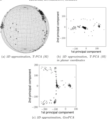
[image:23.612.130.480.191.370.2]variation. In comparison in Figure 8c we adapt Figure 6 from Sargsyan, Wright and Lim (2012). Again the clusters can be well discriminated along the first GeoPC (horizontal in the 2D approximation in Figure8b). In con-trast to T-PCA, however, the data are not well approximated by the first GeoPC, as the projections to the second GeoPC component (vertical in the 2D approximation in Figure8c), feature maximal data range. In fact, both GeoPCs explain roughly similar amounts of data variation.
Thus Figure8illustrates the power of T-PCA going significantly beyond the analysis of Sargsyan, Wright and Lim (2012). Not only can the prese-lected clusters be separated but the data are very accurately approximated by their projection to the 1D component.
3.2. The 1D structure of C2 Data Set. We now describe in detail how our C2 data set is extracted from the large RNA data set. Notably, some of the RNA structures in this data set are only short pieces adhering to a protein or another RNA structure. Therefore, we prune by removing residues further than 50◦ in torus distance from their nearest neighbor. This leads to 7544 residues and 649 of these are residues with C2’-endo sugar pucker. i.e.
ν2 ∈[300◦,350◦]. This produces a moderately large data set to analyze (in
contrast to the very large data set of all other residues including C3’-endo sugar pucker).
Murray et al. (2003) noted that this data set is locally rotameric, as, among others, conformer clusters essentially extend along theβ angle, con-sidering only the 3 heminucleotide angles α−β −γ (Figure 9a). Already in this heminucleotide space, these individual 1D cluster patterns compete with the group spread along theαangle and in full 7D residual space, there are more competing features, which, in the 2D TS-PCA plot involving all 7 angles, manifest as 3 diffused stripe shaped clusters (Figure 9b). Here the 1D pattern of the largest conformer group can be traced along the shifted second diagonal. The two conformer groups next in size, which are close in heminucleotide angles, are ripped apart in TS-PCA due to its wrong topol-ogy, because they are far from the base point of the tangent space that is controlled by the dominating cluster. Notably, the correct topology could not even be forced onto that plot because, due to the winding effects illustrated in Figure1, boundary loci correspond to different torus loci.
Due to its larger flexibility and higher fidelity, T-PCA recovers a 1D pat-tern as the overall dominating structure, reflecting the proximity of the sec-ond and third largest cluster in the 2nd component (Figure 9c, and Figure
(a)2D approximation, T-PCA (SI) (b) 2D approximation, T-PCA (SI) in planar coordinates
(c)2D approximation, GeoPCA
Fig 8:Two-dimensional PCA approximations of the benchmark data set via T-PCA with SI ordering in natural spherical coordinates (8a), in planar coordinates (8b) and GeoPCA adapted from (Sargsyan, Wright and Lim,
2012, Figure 6) (8c). The symbols represent the same clusters as in Figure
7.
due to the large gaps in the β and γ angles, cf. Figure 9a. Using T-PCA, we generalize the finding of a locally rotameric structure by Murray et al.
(2003) to
[image:25.612.131.482.98.491.2](a)Conformer clusters in theα−β−
γ plot adapted from (Murray et al.,
2003, Figure 4.b)
(b)TS-PCA
(c) T-PCA (SI) (d)T-PCA (SI), planar view
Fig 9: Residues with C2’-endo sugar pucker with clustering following Mur-ray et al. (2003). Three-dimensional heminucleotide angles (9a); two-dimensional TS-PCA (9b) approximation; two-dimensional T-PCA (SI) approximation, the small circle gives the 1D approximation (9c); two-dimensional T-PCA (SI) approximation in planar representation (9d).
essentially following a single angle that is a non-linear combination of the original ones, however.
[image:26.612.127.481.118.506.2]re-flects the clustering in the complementary heminucleotide δ−ǫ−ζ angles from (Murray et al.,2003, Figure 4.c, rear part).
3.3. Comparing T-PCA with TS-PCA. We summarize our use of T-PCA and TS-PCA using all 7 angles for the C2 data in Table5a and Figure10a. In 1D, T-PCA captures 73 % of the variance whereas TS-PCA captures only 44 % of the variance. Only when adding a second dimension TS-PCA captures more variance (81 %) than the 1D component of T-PCA. Higher order PCs, both for T-PCA and TS-PCA, explain roughly the same amount of data variance.
To highlight the differences between the two PCA methods, let us consider the example of three points. There is an exactly fitting small circle used by T-PCA. Indeed, if applied to theη–θplot (Figure7a), T-PCA would reduce the three clusters rather accurately to a 1D circle. In contrast, TS-PCA approximates three points only along a straight line in the tangent space and such an approximation is only possible if data lie favorably such as in theη–θ plot, see (Figure7a). Theα–ζ plot (Figure7b), however, illustrates that a 1D approximation for all seven angles is not possible for TS-PCA, while it is possible for T-PCA (Figure8b).
In fact, usually T-PCA requires one dimension less than TS-PCA because
(a)C2 data (b)Simulated simplex data
Fig 10: Scree plots of cumulative variances for T-PCA (SI) compared to TS-PCA.
Table 5
Cumulative variances for T-PCA (SI) and for TS-PCA.
(a)C2 data
Dimension T-PCA (SI) TS-PCA
1 74% 44%
2 83% 81%
3 90% 90%
4 95% 94%
5 98% 97%
6 99% 99%
(b)Simulated simplex data
Dimension T-PCA (SI) TS-PCA
1 39% 18%
2 50% 34%
3 63% 48%
4 77% 62%
5 89% 75%
6 95% 88%
4. Discussion. We have provided a novel framework for torus PCA to perform PCA-like dimension reduction for angular data. Previous attempts have not been satisfactory, because, on the one hand, the geometry featuring dense geodesics leads to severe restrictions for geodesic approaches while, on the other hand, Euclidean approximations disregard periodicity. We have used an adaptive deformation to a statistically benign geometry, allowing for increased and statistically controlled flexibility whilst at the same time guaranteeing structure fidelity. In application to dihedral angles of RNA structures we have validated our method using a classical benchmark data set. Using a C2’-endo sugar pucker residue data set we have given evidence on how T-PCA is better and more meaningful than TS-PCA, and we have illustrated that thesignificant interdependencefound byMurray et al.(2003) in a 3D representation is seen by T-PCA remarkably in 1D.
[image:28.612.140.470.332.434.2]sta-tistical 1D methods for mode detection (e.g.D¨umbgen and Walther(2008);
Schmidt-Hieber, Munk and D¨umbgen(2013);Huckemann et al.(2016)), and this challenge will be taken up in future research.
Acknowledgments. We are grateful to John Kent and J. S. Marron for helpful discussions. We thank Thomas Hamelryck and Jes Frellsen for their valuable comments on this paper and for pointing to the RNAview program for calculation of RNA bonds. Further, we wish to thank Karen Sargsyan for providing details on GeoPCA and on the RNA data used by her and her collaborators.
SUPPLEMENTARY MATERIAL
Supplement A: Data
(doi:COMPLETED BY THE TYPESETTER; .tar.gz). An illustration how to choose data-driven parameters for torus PCA.
Supplement B: Data
(doi:COMPLETED BY THE TYPESETTER; .tar.gz). RNA residue data used for the analysis in this paper.
Supplement C: Implementation
(doi:COMPLETED BY THE TYPESETTER; .tar.gz). Source code of the T-PCA implementation used for this paper.
References.
Altis, A.,Otten, M.,Nguyen, P. H.,Rainer, H.andStock, G.(2008). Construction of the free energy landscape of biomolecules via dihedral angle principal component analysis.The Journal of Chemical Physics128245102.
Arsigny, V., Commowick, O., Pennec, X. and Ayache, N. (2006). A log-euclidean framework for statistics on diffeomorphisms. In Medical Image Computing and Computer-Assisted Intervention–MICCAI 2006924–931. Springer.
Boisvert, J.,Pennec, X.,Labelle, H.,Cheriet, F.andAyache, N.(2006). Principal spine shape deformation modes using Riemannian geometry and articulated models. In Articulated Motion and Deformable Objects346–355. Springer.
Brewer, J. W. (2013). Regulatory crosstalk within the mammalian unfolded protein response.Cellular and Molecular Life Sciences711067–1079.
Chakrabarti, A.,Chen, A. W.andVarner, J. D.(2011). A review of the mammalian unfolded protein response.Biotechnology and Bioengineering1082777–2793.
Chapman, R.,Sidrauski, C.and Walter, P. (1998). Intracellular Signaling from the Endoplasmic Reticulum to the Nucleus. Annual Review of Cell and Developmental Biology14459–485.
Davis, I. W.,Leaver-Fay, A.,Chen, V. B.,Block, J. N.,Kapral, G. J.,Wang, X., Murray, L. W.,Arendall, W. B.,Snoeyink, J.,Richardson, J. S.et al. (2007). MolProbity: all-atom contacts and structure validation for proteins and nucleic acids. Nucleic acids research35W375–W383.
Dryden, I. L.andMardia, K. V.(2016).Statistical Shape Analysis: With Applications in R. John Wiley & Sons.
Duarte, C. M.and Pyle, A. M.(1998). Stepping through an RNA structure: a novel approach to conformational analysis.Journal of Molecular Biology2841465–1478.
D¨umbgen, L.andWalther, G.(2008). Multiscale inference about a density.The Annals of Statistics361758–1785.
Dunbrack, R. L.and Karplus, M.(1994). Conformational analysis of the backbone-dependent rotamer preferences of protein sidechains. Nature Structural & Molecular Biology1334–340.
Egli, M.,Portmann, S.and Usman, N.(1996). RNA hydration: a detailed look. Bio-chemistry358489–8494.
Estarellas, C.,Otyepka, M.,Koa, J.,Ban, P., Krepl, M.and poner, J.(2015). Molecular dynamic simulations of protein/RNA complexes: CRISPR/Csy4 endoribonu-clease.Biochimica et Biophysica Acta (BBA) - General Subjects18501072–1090.
Fletcher, P. T., Lu, C., Pizer, S. M. and Joshi, S. C. (2004). Principal geodesic analysis for the study of nonlinear statistics of shape.i3eTransMedIm23995–1005.
Frellsen, J., Moltke, I., Thiim, M., Mardia, K. V., Ferkinghoff-Borg, J. and Hamelryck, T.(2009). A Probabilistic Model of RNA Conformational Space. PLoS Comput Biol5e1000406.
Gower, J. C.(1975). Generalized Procrustes analysis.Psychometrika4033–51.
Green, P. J.andMardia, K. V.(2006). Bayesian alignment using hierarchical models, with applications in protein bioinformatics.Biometrika235–254.
Hotz, T.and Huckemann, S. (2014). Intrinsic means on the circle: uniqueness, locus and asymptotics.Annals of the Institute of Statistical Mathematics67177–193.
Huckemann, S. F.and Eltzner, B.(2015). Polysphere PCA with Applications. Pro-ceedings of the Leeds Annual Statistical Research (LASR) Workshop 2015.
Huckemann, S.,Hotz, T.andMunk, A.(2010). Intrinsic shape analysis: Geodesic PCA for Riemannian manifolds modulo isometric Lie group actions.Statistica Sinica11–58.
Huckemann, S.andZiezold, H.(2006). Principal component analysis for Riemannian manifolds, with an application to triangular shape spaces.Advances in Applied Proba-bility2299–319.
Huckemann, S., Kim, K.-R., Munk, A., Rehfeldt, F., Sommerfeld, M., Weick-ert, J.,Wollnik, C.et al. (2016). The circular SiZer, inferred persistence of shape parameters and application to early stem cell differentiation.Bernoulli222113–2142.
Jain, S., Richardson, D. C.and Richardson, J. S.(2015). Computational Methods for RNA Structure Validation and Improvement. InStructures of Large RNA Molecules and Their Complexes, (S. A. Woodson and F. H. Allain, eds.)558181–212. Academic
Press.
Jung, S.,Dryden, I. L.andMarron, J. S.(2012). Analysis of principal nested spheres. Biometrika99551–568.
Jung, S.,Foskey, M.andMarron, J. S.(2011). Principal arc analysis on direct product manifolds.The Annals of Applied Statistics5578–603.
Machine83111–123. Springer.
Kent, J. T.andMardia, K. V.(2009). Principal component analysis for the wrapped normal torus model. Proceedings of the Leeds Annual Statistical Research (LASR) Workshop 2009.
Kent, J. T.andMardia, K. V.(2015). The Winding Number for Circular Data. Pro-ceedings of the Leeds Annual Statistical Research (LASR) Workshop 2015.
Laborde, J.,Robinson, D.,Srivastava, A.,Klassen, E.andZhang, J.(2013). RNA global alignment in the joint sequence–structure space using elastic shape analysis. Nucleic acids research41e114–e114.
Liu, W.,Srivastava, A.andZhang, J.(2011). A mathematical framework for protein structure comparison.PLoS Comput Biol7e1001075.
Mardia, K. V.(2013). Statistical approaches to three key challenges in protein structural bioinformatics.Journal of the Royal Statistical Society: Series C (Applied Statistics)62
487–514.
Mardia, K. V.andJupp, P. E.(2000).Directional Statistics. Wiley, New York. Mardia, K. V.,Kent, J. T.andBibby, J. M.(1979).Multivariate Analysis.Probability
and mathematical statistics. Academic Press.
Murray, L. J. W.,Arendall, W. B. I.,Richardson, D. C.andRichardson, J. S. (2003). RNA backbone is rotameric.Proc. Natl Acad. Sci. USA10013904–13909.
Richardson, J. S., Schneider, B., Murray, L. W., Kapral1, G. J., Im-mormino, R. M.,Headd, J. J., Richardson, D. C., Ham, D.,Hershkovits, E., Williams, L. D.,Keating, K. S.,Pyle, A. M.,Micallef, D.,Westbrook, J.and Berman, H. M.(2008). RNA backbone: consensus all-angle conformers and modular string nomenclature (an RNA Ontology Consortium contribution).RNA14465–481.
Sargsyan, K.,Wright, J. and Lim, C.(2012). GeoPCA: a new tool for multivariate analysis of dihedral angles based on principal component geodesics.Nucleic Acids Re-search40e25.
Schmidt-Hieber, J.,Munk, A.andD¨umbgen, L.(2013). Multiscale Methods for Shape Constraints in Deconvolution: Confidence Statements for Qualitative Features. Ann. Statist.411299–1328.
Schneider, B.,Morvek, Z.and Berman, H. M.(2004). RNA conformational classes. Nucleic Acids Research321666–1677.
Seetin, M. G.andMathews, D. H.(2012). RNA structure prediction: an overview of methods.Bacterial Regulatory RNA: Methods and Protocols99–122.
Sommer, S.(2013). Horizontal Dimensionality Reduction and Iterated Frame Bundle and Development. InGeometric Science of Information.Lecture Notes in Computer Science
808576–83.
Srivastava, A.andKlassen, E. P.(2016).Functional and shape data analysis. Springer. ˇ
Cech, P., Kukal, J., Cern`ˇ y, J., Schneider, B. and Svozil, D. (2013). Automatic workflow for the classification of local DNA conformations. BMC bioinformatics 14
205.
Wadley, L. M.,Keating, K. S.,Duarte, C. M.andPyle, A. M.(2007). Evaluating and Learning from RNA Pseudotorsional Space: Quantitative Validation of a Reduced Representation for RNAStructure.Journal of Molecular Biology372942–957.