This is a repository copy of
Scheduling of Smart Factories using Edge Computing and
Clouds
.
White Rose Research Online URL for this paper:
http://eprints.whiterose.ac.uk/138145/
Version: Accepted Version
Proceedings Paper:
Dziurzanski, Piotr orcid.org/0000-0001-9542-652X, Swan, Jerry and Soares Indrusiak,
Leandro orcid.org/0000-0002-9938-2920 (Accepted: 2018) Scheduling of Smart Factories
using Edge Computing and Clouds. In: 1st International Workshop on Trustworthy and
Real-time Edge Computing for Cyber-Physical Systems (TREC4CPS). International
Workshop on Trustworthy and Real-time Edge Computing for Cyber-Physical Systems, 11
Dec 2018 . (In Press)
[email protected] https://eprints.whiterose.ac.uk/
Reuse
Items deposited in White Rose Research Online are protected by copyright, with all rights reserved unless indicated otherwise. They may be downloaded and/or printed for private study, or other acts as permitted by national copyright laws. The publisher or other rights holders may allow further reproduction and re-use of the full text version. This is indicated by the licence information on the White Rose Research Online record for the item.
Takedown
If you consider content in White Rose Research Online to be in breach of UK law, please notify us by
Scheduling of Smart Factories using Edge Computing and Clouds
Piotr Dziurzanski, Jerry Swan and Leandro Soares Indrusiak
Abstract— Reconfiguration-as-a-Service is an emerging trend for dynamic smart factories. This approach exploits cloud-based services to continuously optimise the performance of manufacturing systems. The edge computing paradigm, on the contrary, aims at performing the whole computation at the edge of the network, close to the data sources. In this paper, a trade-off between these two possibilities is analysed. A value-based criterion is proposed for executing optimisation engine either in a cloud or at the edge. Experimental results determine the ranges for both the cloud computation cost and the edge computer’s speed in which manufacturing scheduling leads to higher profits.
I. INTRODUCTION
One of the emerging trends related to smart factories is to migrate some computational tasks (e.g. scheduling of manufacturing processes) from remote clouds in order to be closer to devices that are the source and/or target of such computing, i.e. to the edge between the IoT’s things and the network [1]. One of the key predictions discussed in the IDC report [2] was that in the near future almost half of IoT-created data will be stored, processed, analysed and acted upon at or close to the network edge. This migration is expected to be beneficial in terms of response time, relia-bility, security and cost effectiveness [3]. It may however be argued that whether a certain computation is to be performed in a cloud or at the network edge should be a dynamic decision. That is, it should be based on the predicted gains and costs of both situational alternatives, rather than decided statically without any situational awareness. In Ismail et al [4], Docker containers were proposed to be executed at the edge. The same containers can be executed in a cloud as well (e.g. by using IBM Cloud Functions1) even
in the case of different os/architecture combinations (thanks to the experimental Docker feature namedDocker manifest). Therefore, the decision on where to execute a certain con-tainer can be made dynamically considering the current edge node utilisation or network bandwidth, and also taking into account the urgency of the computation. In most cases, for efficiency and security reasons it may be beneficial to start computation at the edge, since it decreases network traffic and avoids public/shared networks and servers. However, if the computation performed at the edge progresses too slowly, it can be migrated to a cloud. Such approach requires a method to compare the predicted execution time in both edge and cloud. In this paper we follow a method that predicts the benefits of further manufacturing optimisation proposed in ref. [5]. According to that method, each manufacturing order, which requests the production of a particular commodity, is equipped with a value curve, that models the value,
Department of Computer Science, University of York,
Deramore Lane, Heslington, YO10 5GH, York, UK
{piotr.dziurzanski,leandro.indrusiak}@york.ac.uk
1https://console.bluemix.net/openwhisk
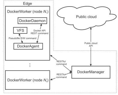
DockerManager DockerWorker (node N1)
DockerWorker (node Nk) DockerAgent
DockerDaemon
VFS Docker API REST command Pseudofile R/W command
...
Public cloud Edge
Public cloud API
RESTful command
[image:2.595.336.533.144.303.2]RESTful command
Fig. 1. General scheme of the proposed approach implementation
expressed in the monetary units, yielded by the manufac-turing order over time. This value curve can influence the optimisation process as follows: since further search-based schedule optimisation is occupied with the cost of the cloud nodes performing the computation, it has been shown in that paper that it may be beneficial (grounded in terms of overall monetary cost) to prematurely stop the optimisation and apply the best results found so far. In this paper, we propose to extend that model with the possibility of performing the optimisation at the network edge. Using the proposed technique, on obtaining a manufacturing order, an agent decides not only when to finish the optimisation process, but also whether the computation should be performed at the edge or in a cloud, comparing the predicted monetary gains for all these options.
II. PLATFORM AND APPLICATION MODEL
The class of scheduling problems analysed in this paper concerns manufacturing in which the value gained by an end-user depends on both optimisation solution quality and the time taken by the optimisation process itself. The optimisa-tion process is performed either at the network edge or in a cloud. Suitable application and platform models are proposed below.
A. Platform model
At the network edge, there is a set ofkcomputing nodes
N = {N1, . . . , Nk} capable of executing one or more
containers (i.e. each node runs a typical Docker container engine). The nodes are heterogeneous and their response time difference is expressed with so-calledcalibration coefficient
ζx,x∈ {1, . . . , k}.ζxdenotes the ratio between empirically
time t value V
AT D
0
ET
Vmax
VC(t)
VC(ET)
[image:3.595.90.268.53.142.2]Z
Fig. 2. An example value curve of manufacturing orderO
a public cloud serving as an alternative execution platform, as shown in Fig. 1 (the details of this figure are explained later in this paper). The benchmarks’ response times on a reference unit include the communication cost and the container initialisation time.
In ref. [5], it was assumed that the schedule optimisation engine was containerised and executed in a public cloud using a function as a service facility, which significantly reduced the initialisation time and monetary cost, in com-parison with the more prevalent Containers as a Service paradigm. However, such containers can also be executed at the edge of the network, potentially decreasing the opti-misation cost. Only when it is predicted that further local optimisation at the edge is likely to be less beneficial than remote execution, are the containers migrated and executed in the cloud.
B. Application model
The application considered in this paper is related to manufacturing scheduling optimisation in a smart factory. At time instants not known a priori, manufacturing orders are submitted. Each of these orders usually concerns the production of several items of a certain product. The role of optimisation is to allocate the manufacturing processes (such as mixing powders, cutting parts etc.) to different machines, select the most appropriate machine modes (e.g. thereby trading production time against energy efficiency) and schedule these processes in time, following the depen-dency relation between these processes. As discussed for example in ref. [5], such optimisation problems are NP-hard and thus various search-based heuristics are usually applied to find an approximate solution.
Each optimisation process is performed dynamically and concurrently to the manufacturing of the previous orders. Consequently, optimisation results must typically be pro-vided within a limited time span. As long as the factory is busy with the previous orders, the optimisation time does not matter. However, in the case of an idle factory, the time spent on optimisation incurs ongoing factory maintenance costs due to idleness. This phenomenon is well illustrated with the value curve presented in Fig. 2. At time instantAT
a manufacturing order is submitted. The maximal possible profit from this order is equal toVmax, defined as the excess of revenue over cost and denoted in monetary units. As the factory is busy up to time instant D, processing orders submitted and scheduled earlier, the profit value does not change in interval [AT, D). However, after D, the profit value decreases up to a certain point Z, where it reaches 0. If the optimisation process ends at timeET, the maximal
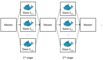
Master Master Master ...
1ststage 2ndstage
Slave S1,1
Slave S1,2
Slave S1,p
Slave S2,1
Slave S2,1
Slave S2,p
... ...
1 2
Fig. 3. Stages of the optimisation process
potential profit cannot exceed the value of the curve atET, namelyV C(ET).
III. OPTIMISATION TRADE-OFFS
The scheduling optimisation is performed in a master-slave fashion as illustrated in Fig. 3, in sequential stages indexed with i = 1,2, . . .. At each i-th stage, a set of pi containers is executed in parallel by slave nodes. The global master coordinates the execution of containers submitted by the users. The master is responsible for serving the incoming requests and allocates the containers to nodes, for example using the algorithms proposed in ref. [6].
All containers Si,y, y ∈ {1, . . . , pi}, are executed either in a cloud or at the network edge. Each container gets the encoded manufacturing order together with the best solutions found so far as its input and after time ti,y returns the minimal value found by the optimisation for the manufactur-ing cost of that order,fi,y, together with the corresponding solution.
If Si,y is executed on edge node Nx, its CPU time slot is proportional to the so-called CPU shares ξi,y ∈
{1, . . . ,1024} (the value of the maximum share is taken
directly from the Docker’s–cpu-sharesflag). Assuming that the sum of all the CPU shares of containers executed on nodeNx equalsΞx, containerSi,y gets ϑi,y,x=ξi,y/Ξx of the CPU time of nodeNx.
Initially, the execution time of the containersSi,y is diffi-cult to be predict accurately. However, as all these containers are constructed from the same container image and perform optimisation of the same problem size, the workload inside these containers is similar. Thus the response time ti,y of each containerSi,y can be measured and used by the master node to predict the future response times at the following stages, as described subsequently.
Due to the change of a potential maximal profit from a certain manufacturing order over time as described by a value curve, a clear trade-off between the optimisation time and the optimisation quality can be identified. As a search-based heuristic keeps the best result found so far and continuously explores the search space up to the fulfilment of a certain stopping criterion, it can provide a sub-optimal result at any time. For example, ref. [5] proposed that for the master-slave architecture introduced earlier (Fig. 3), after the i -th stage -the master node ga-thered -the optimisation results
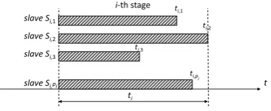
[image:3.595.349.522.54.155.2]t i-th stage
slave Si,1
slave Si,2
slave Si,3
slave Si,pi
ti
ti,1
ti,2
ti,3
ti,p
[image:4.595.79.277.53.134.2]i
Fig. 4. Stage execution time example
Performing the optimisation at the edge is assumed to cost nothing in terms of money as the edge devices are owned by the smart factory and their idle time can be viewed as wasted. This is in contrast to the optimisation cost in a cloud, which for anyi-th stage is nonzero and upperbounded with
β·ti·pi, whereβ is the cost of a single container execution per one time unit2, p
i is the number of slaves executed at thei-th stage andti = maxy∈{1,...,pi}(ti,y)(see Fig. 4). The
execution cost in both these locations can be described with equation
ci= ∆i·(β·ti·pi), (1)
where ∆i equals 1 if the i-th stage is executed in a cloud or 0 otherwise. Using these notations, the manufacturing profit yielded by the best solution found in thei-the stage is described with equation
Pi=V C
i
X
j=1
tj
−
i
X
j=1
cj−fi, (2)
wherefi= miny∈{1,...,pi}(fi,y).
After finishing the optimisation process at stage i, the values of ti+1 andfi+1 can be predicted via extrapolation,
for example using the Bluirsch and Stoer algorithm [7]. For history lengths of 3 or less, such extrapolation is either undefined or else the result was empirically determined to be inaccurate: the predicted value offi is then given by the best fitness found so far and that of ti by the last (actual) processing time.
If the following,(i+ 1)-th stage is processed at the edge, valueteˆi+1 predicts its execution time andfˆi+1 predicts the
lowest value returned by the slaves. Both these values can be used to predict the profit generated at the edge after the subsequent stage as follows
ˆ
P ei+1 =V C
i
X
j=1
tj+ ˆtei+1
−fˆi+1−
i
X
j=1
cj. (3)
Let us assume that at thei-th stage, executed at the edge, the longest computation (lasting ti) has been performed by the x-th node with calibration coefficient ζx and whose fraction of CPU time for the related container equalsϑi,y,x. This container is predicted to be executed for teˆi+1 in the
following stage if executed at the edge. Then the execution time in a cloud of the same container can be assessed with formula
2For exampleβ= 0.000017USD per second of execution per GB of memory allocated using IBM Functions in August 2018.
ˆ
tci+1=
ˆ
tei+1
ζx·ϑi,y,x
(4)
Then the profit generated after the subsequent stage exe-cuted in a cloud can be estimated with equation
ˆ
P ci+1=V C
i
X
j=1
tj+ ˆtci+1
−fˆi+1−
i
X
j=1
cj−cˆi+1. (5)
If the current, i-th stage is executed in a cloud, the execution time of the following stage at the edge can be assessed with equation
ˆ
tei+1= ˆtci+1·ζx·ϑi,y,x, (6)
and substituted to equation (3) to estimate the corresponding profit. Value tcˆi+1 is also used to estimate ˆci+1 using
equation (1).
The stopping criteria are evaluated by the master node after each stage i. Thepredicted profit criterion checks the prediction if the execution of the subsequent stage is likely to increase the profit generated by the optimised process or not, regardless it is executed in a cloud or at the edge
Pi>max( ˆP ei+1,P cˆ i+1). (7)
Moreover, if P eˆ i+1 ≥P cˆi+1, the following stage should
be executed at the edge. Otherwise, the containers shall be executed in a cloud.
The benefits of similar stopping criteria in a cloud envi-ronment has previously been evaluated [5]. In the following section, we apply this approach to a platform consisting of both edge machines and a cloud.
IV. EXPERIMENTAL RESULTS
The edge execution platform described above has been im-plemented and used together with the original Docker engine in form of two software modules, namely DockerManager
andDockerWorker. The former one corresponds to the master
node and is run on a machine where Docker may or may not be installed, whereas the latter, executing the slave nodes, requires the presence of the Docker daemon. These modules are depicted in Fig. 1.
In order to evaluate the technique described in this paper, 30 manufacturing orders considered in ref. [5] have been selected to be scheduled in a certain factory. In that factory, there are 8 machine types and each machine can operate in different operating modes, influencing both the processing time and the consumed energy, which in turn influences the manufacturing cost. The number of manufacturing process steps in these orders ranged from 18 to 59. Each of these steps needs to be allocated to a machine operating in a certain mode. The parameters for the associated value curve are
AT = 0, D = 250 s, Z = 500s and Vmax = 5000 GBP, which means that such amount of money would be gained by a plant if both the production and the scheduling cost nothing.
0.1 0.3 0.5 0.7
0.9 1.1 1.3 1.5 1.7 1.9
-10000 -8000 -6000 -4000 -2000 0 2000 4000
0.500000 0.062500 0.007813
0.000977 0.000122
0.000015 0.000002
Average calibration coefficient x
P
ro
fi
t d
if
fe
re
n
ce
b
e
tw
e
e
n
e
d
g
e
an
d
c
lo
u
d
e
xe
cu
ti
o
n
[
G
B
P
[image:5.595.52.299.55.184.2]]
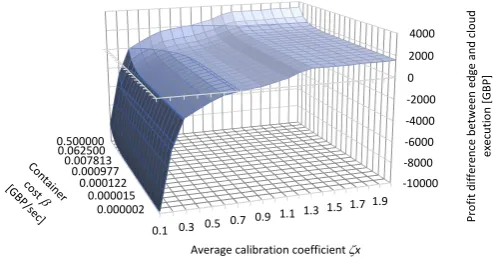
Fig. 5. Profit difference between edge and cloud execution for various average calibration coefficient values and container execution costs
is then performed using the same platform, edge or cloud, from the first stage up to the computation completion. The average calibration coefficientζx ranges from 0.1 (response time from the edge is 10 times longer than from cloud) to 2.0 (response time from the edge is two times faster than from the cloud), and the container execution cost per second, β, varied from 0.000001 GBP to 0.5 GBP. For each setting, the experiment has been conducted 100 times, 400000 runs in total. The difference between the total profit computed in the edge and in the cloud are presented in Fig. 5. Not surprisingly, the time needed for optimisation in case of slow edge computers (i.e. with low average calibration coefficient
ζx) causes that the computation is usually finished at the time when the associated value curve assumes low values. For extreme case of edge machines with, on average, 10 times lower response time than a cloud (average ζx equals 0.1), even assuming the most expensive cloud computation cost (β equals 0.5GBP) leads to high total differences in profits (close to 10000 GBP for the considered set of orders). However, with the increase of the edge machine speed, this difference changes significantly. Assuming typical cloud computation cost in 2018 β = 0.000015 GBP, edge computations becomes slightly more beneficial (107 GBP difference) for averageζx equal to 0.8. For the fastest edge computers considered, with a response time twice as fast as cloud computers, this difference is equal to almost 1600 GBP. As a similar value is achieved even for much cheaper cloud computation (β= 0.000001GBP), this proportion will hold even after the forseeable significant decrease in cloud computation cost. In total, processing in edge returned above 8% higher profit than computation in a cloud.
In the next experiment, the slave container migration between edge and cloud is permitted. The computation starts at the edge but migrates to a cloud if the predicted profit of the next stage computed in a cloud is higher than its equivalent predicted for the edge. In the analysed range, the number of migrations from the edge to cloud depends strongly on theζxparameter and to a lower degree onβ. For the slowest cloud (ζx= 0.1), the migration from the edge to the cloud has been performed in 51% of cases on average, and then decreases almost linearly to 13% for ζx = 1.0, i.e. when both the edge and cloud have the same response time on average. For faster edge (ζx > 1.0), not a single migration has been observed. For all the considered cases, the
possibility of migration to cloud improved the profit slightly, yielding 1% above the execution in edge and 9% higher profit than computation in a cloud. However, this option is more beneficial in case of slow (or busy) edge. For the slowest case (ζx = 0.1), computation performed solely at the edge yields 22% worse result than a cloud, whereas the possibility of migrations decreases this gap up to 14%. The migration option may be then viewed as quite beneficial in adverse situations, which remains unused in case of a higher computational power available at the edge.
V. CONCLUSION
This article describes a distributed architecture that pro-vides general and scalable support for the ‘Just in Time’ manufacturing process envisioned for smart factories. The architecture is equipped with a novel adaptive stopping criterion for optimising profit obtained from a set of man-ufacturing orders which not only decides on the computa-tion terminacomputa-tion but also steers the computacomputa-tion migracomputa-tion between the edge and cloud. As the optimisation engine has been encapsulated into a stateless container, such mi-gration is occupied with a minimal overhead. According to the experimental results, optimisation at the edge leads to a slightly better overall profit, and in case of slow or busy edge computers, the possibility of container migration to cloud decreases the computation speed gap between a cloud and edge. Since using the proposed approach leads to comparable if not better profits than optimisation solely in a cloud, considering the additional benefits form edge execution, such as reduction of outbound/inbound network traffic, increased reliability and security, edge platform can be viewed as a promising alternative to cloud computing even for computationally costly tasks.
ACKNOWLEDGEMENT
The authors acknowledge the support of the EU H2020 SAFIRE project (Ref. 723634).
REFERENCES
[1] D. Tamburini. (2018) Enabling smart manufacturing with edge computing. [Online]. Available: https://azure.microsoft.com/en-gb/blog/enabling-smart-manufacturing-with-edge-computing/
[2] M. Carrie, V. Turner, R. Yesner, J. Feblowitz, K. Knickle, L. Lamy, M. Xiang, A. Siviero, and M. Cansfield. (2016) Idc futurescape: Worldwide internet of things 2016 predictions. [Online]. Available: https://www.idc.com/research/viewtoc.jsp?containerId=259856 [3] H. El-Sayed, S. Sankar, M. Prasad, D. Puthal, A. Gupta, M. Mohanty,
and C. Lin, “Edge of things: The big picture on the integration of edge, iot and the cloud in a distributed computing environment,”IEEE Access, vol. 6, pp. 1706–1717, 2018.
[4] B. I. Ismail, E. M. Goortani, M. B. A. Karim, W. M. Tat, S. Setapa, J. Y. Luke, and O. H. Hoe, “Evaluation of docker as edge computing platform,” in 2015 IEEE Conference on Open Systems (ICOS), Aug 2015, pp. 130–135.
[5] P. Dziurzanski, J. Swan, and L. S. Indrusiak, “Value-based manufacturing optimisation in serverless clouds for industry 4.0,” in
Proceedings of the Genetic and Evolutionary Computation Conference,
ser. GECCO ’18. New York, NY, USA: ACM, 2018, pp. 1222–1229. [Online]. Available: http://doi.acm.org/10.1145/3205455.3205501 [6] P. Dziurzanski and L. S. Indrusiak, “Value-based allocation of docker
containers,” in2018 26th Euromicro International Conference on
Par-allel, Distributed and Network-based Processing (PDP), March 2018,
pp. 358–362.
[7] J. Stoer, R. Bartels, W. Gautschi, R. Bulirsch, and C. Witzgall,
In-troduction to Numerical Analysis, ser. Texts in Applied Mathematics.