Review
Heat transfer of a buoyancy-aided turbulent flow in a trapezoidal
annulus
Y. Duan
a,b, S. He
a,⇑aDepartment of Mechanical Engineering, University of Sheffield, Sheffield S1 3JD, UK b
School of Mechanical, Aerospace and Civil Engineering, University of Manchester, Manchester M13 9PL, UK
a r t i c l e i n f o
Article history:
Received 18 October 2016
Received in revised form 27 April 2017 Accepted 15 June 2017
Available online 22 June 2017
Keywords:
Mixed convection Buoyancy-aided flow Heat transfer
Non-uniform flow passage Rod bundle
Large flow structures
a b s t r a c t
The objective of this paper is to report a numerical investigation into the heat transfer of a buoyancy-aided flow in a rod-bundle-like channel. The flow field is simulated using large eddy simulation (LES) with WALE SGS model and the buoyant force is taken into account using the Boussinesq approximation. The general trend of the effect of buoyancy on the overall heat transfer is similar to that in a pipe flow, but the effect on the regional heat transfer varies greatly. This has resulted from a number of interplaying factors, including, the redistribution of the mass flow in the various sub-channels, the non-uniform buoy-ancy effects on turbulence in different regions of the domain and the behaviour of the large flow struc-tures in the flow channel. These factors together make the effect of buoyancy on heat transfer in the considered flow channel really complicated, while the last factor has been found to have the most pro-nounced effect in most cases studied.
Ó2017 The Authors. Published by Elsevier Ltd. This is an open access article under the CC BY license (http:// creativecommons.org/licenses/by/4.0/).
Contents
1. Introduction . . . 211
2. Methodology. . . 213
2.1. Computational domain . . . 213
2.2. Numerical methodologies and cases . . . 213
3. Results and discussions . . . 214
3.1. Temperature field and teat transfer results . . . 215
3.2. Buoyancy effects on the regional flow . . . 215
3.2.1. The mean velocity . . . 215
3.2.2. Turbulence quantities. . . 216
3.2.3. Production of turbulent kinetic energy . . . 218
3.3. Buoyancy effect on the large flow structures: a statistic view . . . 221
4. Conclusions. . . 223
Conflict of interest . . . 223
Acknowledgements . . . 223
References. . . 223
1. Introduction
Mixed convection is encountered in many engineering applica-tions, including for example, nuclear reactors and electronic heat
exchangers. Dependent on the directions of the buoyancy and flow, the mixed convection in a vertical channel is referred to as buoyancy-aided or -opposite convection. In buoyancy-aided convection, the body force is in the same direction as the heated flow, while it is opposite in the other case. Many efforts have been devoted to this field in the past decades. Petukhov and Poly-akov [1] and Jackson et al. [2] provide summaries of the early
http://dx.doi.org/10.1016/j.ijheatmasstransfer.2017.06.070
0017-9310/Ó2017 The Authors. Published by Elsevier Ltd.
This is an open access article under the CC BY license (http://creativecommons.org/licenses/by/4.0/).
⇑ Corresponding author.
E-mail address:s.he@sheffield.ac.uk(S. He).
Contents lists available atScienceDirect
International Journal of Heat and Mass Transfer
work from the 1960s to 1980s. A recent review is provided by Jackson[3].
It has been observed in many experimental studies that the effect of buoyancy can either improve or reduce heat transfer rate. It depends on the flow direction, thermal loading and the charac-teristics of the flow (laminar or turbulent). Considering the laminar flow first, heat transfer is enhanced in a buoyancy-aided flow. This can be explained by the stronger advection due to the accelerated velocity in the near wall region. By contrast, the heat transfer rate is impaired in the buoyancy opposite convection because the velocity near the heated surface is decelerated. In a turbulent flow, the buoyancy effect on heat transfer is more complicated. In a buoyancy-opposed flow, the buoyant force causes an increase in shear stresses near the wall, which in turn results in more turbu-lence to be generated and hence heat transfer improvement, despite that the velocity decreases in the near wall region. The sit-uation is more complex in the buoyancy-aided case. The flow is firstly laminarized by the body force when the heat flux is small. The laminarization effect becomes more remarkable when the heat flux is increased. This continues until the flow is completely lami-narized at certain heat flux which causes most severe heat transfer impairment. When the heat flux is further increased, turbulence is regenerated in the flow, and hence heat transfer recovers. Conse-quently, heat transfer in the buoyancy-aided flow can be divided into laminarizing regime and recovery regime depending on the effect of body force on turbulence. Both the turbulence and heat transfer coefficient reduce with increasing heat flux in the laminar-izing region, but they increase with the increase of heat flux in the recovery regime.
Rouai[4]presented a refinement of the correlation original pro-posed by Jackson and Hall[5]. The correlation is to evaluate theNu
of a fully developed turbulent mixed convection in a uniformly heated vertical passage:
Nu Nuf
¼ 18104Bo Nu
Nuf 2
!0:46
ð1Þ
where the negative and positive signs are for buoyancy-aided and buoyancy-opposite convection, respectively.NuandNuf are Nusselt
numbers for the mixed convection and forced convection, respec-tively.Bo is the buoyancy parameter to quantify the strength of buoyancy force, which is defined as:
Bo¼ Gr
Re3:425Pr0:8 ð2Þ
whereReis the Reynolds number, Pris the Prantl number of the fluid, andGris Grashof number based on heat flux:
Gr¼gbD 4
hq
k
m
2 ð3ÞThere is a discontinuity in Eq.(1) for the buoyancy-aided mixed convection flow, which occurs atBo3106. TheNudecreases with the increase ofBowhenBo<3106, but increases mono-tonically whenBo>3106.
With the development of computer technology, computational fluid dynamics (CFD) has now become a very useful tool in the study of flow and heat transfer phenomena. According to the review of Jackson et al.[2], the first attempt to use CFD to investi-gate mixed convection dated back to early 1960s, e.g., Hsu and Smith [6]. Walklate [7] firstly demonstrated that low-Reynolds number turbulence model proposed by Jones and Launder[8]can predict the heat transfer with reasonable accuracy. In the following decades, several low Reynolds number turbulence models have been found to perform well in the prediction of mixed convection in the vertical pipe by a number of authors[9–13]. A systematic study was carried out by Kim et al.[14]to assess the performance of a number of turbulence models including Launder-Sharma[15], Chien[16], Lam-Bremhorst[17], Abe-Kondoh-Nagano[18], Wilcox
[19], Yang-Shih[20], Myoung-Kasagi[21], Hwang-Lin[22],V2-Fby Behnia et al.[23]and Cotton-Kirwin [24]. It was found that the Launder-Sharma model and Yang-Shih model are the best in terms of reproducing the general trend of buoyancy influence in the ver-tical turbulent mixing convection. Thanks to the fast development of the computer technology, direct numerical simulation (DNS) of mixed convection becomes possible. In Kasagi and Nishimura
[25]and You et al.[26], DNS was used to simulate laminar and tur-bulent mixed convection in a vertical channel. Properties of
work-k turbulent kinetic energy,ðw02þu02þ
v
02Þ=2 (m2/s2)Nu Nusselt number,hDh/k
Nuf Nusselt number in the force convection case Nuloc local Nusselt number,hlocDh/k
P/D pitch to diameter ratio
Pr Prantl number
qw averaged heat flux on the walls (W/m2) qloc local heat flux on the walls (W/m2) Re Reynolds number,UbDh/
t
S the size of the narrow gap (m)
Sij strain rate tensor (1/m) Twall wall temperature (K)
Tbulk bulk temperature (K);
Ub bulk velocity (m/s)
b
k thermal conductivity (W/m K) h angles on the rod wall (°)
l
dynamic viscosity (kg/m s)t
kinetic viscosity,l
/q
(m2/s)Acronyms
CFL Courant-Friedrichs-Lewy condition or number LES large eddy simulation
LES_IQv the LES quality criteria proposed by Celik et al.[62,63] RANS Reynolds-averaged Navier-Stokes
ing fluids in both studies were treated as constants, while the buoyancy effect was simulated using the Boussinesq approxima-tion. DNS can reveal much more details about the flow in compar-ison with experiments, but it requires very high computing resources and can only be used for low Reynolds flows with simple geometry. Large eddy simulation (LES) is an alternative, which can achieve a reasonable accuracy while being less expensive than DNS as demonstrated in[27,28].
Compared with the enormous number of papers on mixed con-vection in uniform geometries, like tubes, channels, and concentric annulus, there are much fewer papers on a non-uniform geometry, such as a rod bundle or an eccentric annulus. Even less attention was paid to the turbulent mixed convection in a heated non-uniform geometry. According to the best knowledge of the present authors, only two papers considered such flows, namely Chauhan et al.[29] and Forooghi et al. [30]. Chauhan et al. adopted the
SST-
x
model to investigate the buoyancy-aided flow in an annulus with various radial ratios and eccentricities. Heat transfer results were reported. In the article by Forooghi et al.,V2-Fmodel was used to investigate the turbulent buoyancy-aided flow in a concen-tric and various eccenconcen-tric annuli. It was revealed that heat transfer deterioration is less significant in the buoyancy-aided flow in an annulus with a higher eccentricity than that with a lower eccen-tricity. It was also found that the flow in the narrow gap was faster than in the big gap when the heat flux was sufficiently high. In addition, the reduction of turbulent kinetic energy due to buoy-ancy is much weaker in the narrow gap than in the wide part of the channel. Due to the use of a steady solver in their study, the large unsteady flow structures in the narrow gaps which are expected were not simulated. Such flow structures were demon-strated to exist in eccentric annuli under isothermal and forced convection conditions by several authors. Initially found by Hooper and Rehme[31]and latterly confirmed by other authors[32–40], such flow structures exist in the vicinity of narrow gaps formed by tightly packed rods and are deemed to be the reason of the high turbulence quantities observed in the region. Similar flow phe-nomenon has also been observed in other types of non-uniform channels, referring to[41–58]. Geometries that have been consid-ered include a trapezoid/rectangular channel with a rod mounted in it, eccentric annular channels with a high eccentricity, and chan-nels containing/connected by a narrow gap. Large flow structures can exist in both laminar and turbulent flows in such non-uniform geometry configurations, while the behaviour of them is mainly dependent on the geometry configure. In particular, the Strouhal number of the large flow structures is governed by pitch-to-diameter ratio (P/D) or gap-to-diameter ratio under the isothermal or forced convection conditions. The first attempt to use CFD to study flow structures in a non-uniformly geometry is dated back to the late 1990s, refer to[51]. As confirmed by many authors[52–54], the URANS can reproduce some flow behaviours but with less accuracy compared to LES. Experimental investiga-tions on the natural convection, forced convection and mixed con-vection under small buoyancy force in concentric and eccentric annulus with various eccentricities were reported in[55–57]. The eccentricity caused a reduction in heat transfer rate in comparison with that in a concentric annulus. In case of forced convection, the distribution of the local heat transfer rate of the rod is increasingly more uniform as the annulus eccentricity increases from 0.5 to 0.9, refers to[57]. It was also suggested that the existence of the large flow structures improved mixing in the channel.Buoyancy force is unavoidable in nuclear reactors under certain conditions, especially under some hypothetic fault conditions. It is deemed to be more relevant in some concepts of the Gen IV nuclear reactors, such as the supercritical water reactor (SCWR). The fuel rods in the bundles in the concept of (SCWR) are closer to each other than their counterparts in other types of the nuclear reactors
such as PWRs and AGRs. Subsequently, large flow structures are more likely to occur in such designs. According to the best knowl-edge of the authors, there has not been any study to characterise the large flow structures in buoyancy-influenced flows in a non-uniform channel, except for the recent paper by the current authors[58]. It was demonstrated in[58]that large flow structures exist in both the larger and smaller gaps formed by a rod and trapezoid channel similar to the experimental facility of Wu and Trupp[41,42]. The considered configuration (trapezoidal annulus) is a simplified case for the tightly-packed triangular-array rod-bundle in the nuclear reactor. The influences of buoyancy on the features of the flow structures were discussed in the paper[58]. In the forced convection concerned, the flow was found to swing from one side of the main channel to the other side through the narrow gap. The Strouhal number based on bulk velocity matched closely with the experimental results of Wu and Trupp[41,42]in a similar geometry, despite the Reynolds was much higher in their experiments. This finding supports conclusions by other authors that the St1of the large flow structures in a narrow gap is mostly
related to the geometry once the Reynolds number is sufficiently high. The buoyancy effect on the St1has similar a trend as the
effect on the overall heat transfer. The mixing velocity due to such flow structure reduces with the increase of the buoyancy force, whereas a visible decrease in the horizontal size of the flow struc-tures was observed in the turbulence recovery case. There are also large flow structures in the wide gap of the flow passage, despite being very weak in the forced convection case. These flow struc-tures are enhanced by buoyancy, especially in the turbulence recovery case. The early paper[58]focused on mean flow struc-tures. The purpose of this paper is to report heat transfer and tur-bulence results of the same simulations. We discuss the effects of buoyancy on heat transfer and report overall and local heat trans-fer results, flow statistics and the turbulence quantities, in order to provide a better understanding of buoyancy influenced flow, which will assist the design and safety analysis of advanced nuclear reactors.
2. Methodology
2.1. Computational domain
The geometry of the flow cross-section in the current study is the same as that considered in the experiment by Wu and Trupp
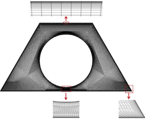
[41,42]. It is formed by a trapezoidal channel enclosing a rod in it as shown in Fig. 1. The diameter of the rod is d = 50.8 mm, and the height of the trapezoid wall is 66.0 mm. The lengths of the short and long edges of the trapezoid are 50.8 mm and 127.0 mm, respectively. The height of the narrow gap g = 4 mm, whereas the height from the top of rod to the long edge of the trapezoid bound (s) is 54.8 mm, which gives a ratio of s/d = 1.08. The hydraulic diameter of the channelDh= 31.4 mm. The whole computational domain extrudes 10Dh long. It was demonstrated in[58]that such the domain used was sufficiently long to capture more than one wave of large flow structures in both forced and heat transfer impairment cases. In addition, the X-direction is referred to as the spanwise direction, Y-direction as the transverse direction, and Z-direction as the streamwise direction in the fol-lowing discussion.
2.2. Numerical methodologies and cases
particularly interested in developing a better understanding of the buoyancy effects on heat transfer of flow in the considered chan-nel, and consequently employed Boussinesq approximation to iso-late the buoyancy effect from other variable property effects, as have done previously in many other studies, e.g.,[14,26,28]. The subgrid scale viscosity is modelled by using the wall-adapting local eddy-viscosity (WALE) model. By describing the subgrid scale vis-cosity as a function of the strain and rotation rates, the WALE model has been shown to perform well in shear flows with com-plex geometries. Furthermore, the subgrid viscosity naturally goes to zero at the wall in WALE, as demonstrated by Nicoud and Ducros
[59]. This allows the subgrid scale (SGS) viscosity to be damped in the near wall region as does in a dynamic model. In fact, the WALE model is more stable than dynamic models because it always gen-erates a positive SGS viscosity, while negative values can be gener-ated by dynamic models due to the dynamic procedure. Since the flow in the near wall region is resolved by the LES, a relatively fine mesh is required. A mesh with non-uniform element sizes has been generated. The grid size is smaller in the near wall region than in the main channel. The first near wall mesh resolutions, calculated in Case 1, are in the ranges of 56Dxþ617, 0:136yþ60:2 and 106Dzþ616. There are at least 15 cells located between the wall andyþ= 20. A cross-sectional view can be found inFig. 2. There are about 30,000 cell elements in a radial-circumferential cross sec-tion. Vertically, there are 257 divisions. The whole computation domain contains 7.74 M elements in total. The filtered Navier-Stokes equations and the energy equation are discretized by the bounded central differencing scheme and the second order upwind scheme respectively. The SIMPLE scheme is used for the coupling of the pressure and velocity. The time step,Dtis 0.0001 s, corre-sponding to a CFL (Courant-Friedrichs-Lewy) numberUbDt/Dz of 0.2, whereUbis the averaged bulk velocity.
Simulation cases.An air-like fluid is chosen as the working fluid. The density, specific heat, thermal conductivity, and viscosity are 1.225 kg/m3, 1006.42 J/kgK, 0.0242 W/mK and 1.7894105kg/ ms, respectively. The Reynolds number is approximately 5270 which is about a tenth of that in the experimental study done by Wu and Trupp[41,42]. Four cases have been studied to investigate the effect of buoyancy. The first case is a forced convection flow omitting the buoyancy completely (referred to as ‘Case 1’), while the other cases include the buoyant force, and are hence buoyancy-influenced cases (referred to as ‘Case 2’, ‘Case 3’ and ‘Case 4’). Thanks to the Boussinesq approximation, the fluid prop-erties remain the same in all cases. To activate the buoyancy force, the thermal expansion coefficient is set as 0.001 K1 while the
gravity acceleration is 9.8 m/s and opposite to the flow direction in all of the buoyancy influenced cases. Both the side walls and the tube wall are heated in the buoyancy cases. The temperatures of all of the walls are set to be the same constant, being 800 K,
650 K 1427 K and 6250 K in Cases 1, 2, 3 & 4, respectively. It is noted that because of the use of the air at atmosphere pressure as the working fluid, the wall temperatures in Cases 3 & 4 appear to be unrealistically high. However, when the values are converted to reactor coolant, the wall temperatures would be realistic. In fact, under the Boussinesq assumption, the absolute temperature is not particularly relevant; choice of the temperature values are to achieve a range of values of the buoyancy parameterBo, which were 1.5106, 2.4106and 1.7105in Cases 2–4, respec-tively. Thanks to the Boussinesq approximation and the constant fluid properties, the flow may be fully developed downstream the channel. As a result, the flow may be simulated using a streamwise-periodic condition. In addition, as suggested by Patan-kar et al.[60], a properly scaled temperature also obeys a periodic condition across a defined length of the domain. A scheme for peri-odic thermal boundary condition following this method has been inbuilt in Fluent[61]. In the present work, the periodic boundary condition is applied to both the flow and thermal fields in the flow direction (namely at the inlet and outlet) to simulate a fully devel-oped flow. In order to calculate the scaling of the temperature for the fully developed flow, the upstream bulk temperature was specified.
3. Results and discussions
[image:4.595.308.546.67.262.2] [image:4.595.52.265.67.205.2]Since there is a lack of experimental results or DNS results on flows in a similar passage concerned here, the quality of the simu-lations is checked by using the criteriasandLES_IQvsuggested by Celik et al.[62,63]in Duan and He[58], which demonstrated that a good quality of the simulations has been achieved. Large flow structures were found to be presented in the flow channel in all of the considered cases. In particular, the flow in the vicinity of the narrow gap swings from one side to another, which brings the cooler fluids into/out of the region. The existence of such swinging flow structure is deemed to enhance the heat transfer by helping the fluid mixing. The significance of the buoyancy effects on the behaviour of the large flow structure was discussed in the previous paper[58]. The buoyancy effect on the heat transfer in this non-uniform channel is expected to be more complex than that in a pipe. In the following discussion, heat transfer results, including the overall and local Nusselt number on the walls, are first considered. This is followed by discussion on the effects of buoyancy on the regional flow fields. The flow structures in the Fig. 1.Cross-sectional view of the trapezoidal annulus.
narrow gap are studied using flow statistics. Lines ‘P1’, ‘P2’, ‘P3’ and ‘ML’ are defined in the domain for the presentation of local results (seeFig. 3).
3.1. Temperature field and teat transfer results
The contours of the averaged temperaturehTi/Twallof the
vari-ous cases are presented inFig. 4. The fluid temperature is higher when the flow passage is narrow, lower as flow passage is wider. The average temperature distribution becomes more uniform as theBo⁄increases. Taking the temperature contours of Case 3 & 4 as an example, thehTi/Twallin the main channel is higher than that
in the forced convection case, while thehTi/Twallin the wider gap of
Cases 3 & 4 is lower. The Nusselt number of the forced convection (Nuf) of Case 1 is shown inFig. 5(a), together with the DNS result of forced convection in a heated pipe at a similar Reynolds number (5300) by You et al.[26], the RANS modelling of the DNS flow using the Launder-Sharma (LS) model by Kim et al.[14]. There is some similarity between the current considered geometry and the eccentric annulus in[55–57]. For the case of an annual eccentricity (e) of 0.745, the S/D of the geometry is about 1.08, which is similar to that flow passage in our study. Subsequently,Nuof flow with a similar Re (5450 & 5700) in the annulus with e = 0.7 & 0.8 in
[56,57] are also plotted in Fig. 5(a). Fig. 5(b) shows the Nusselt number ratioNu/Nufof the mixed convection cases of the present study together with those of the DNS as well as of the Launder-Sharma modelling by Kim et al.[14]. It can be seen inFig. 5(a) that the Nusselt number of the forced convection in the current geom-etry is similar to the value obtained using DNS and LS of ascending flow in a heated pipe. The current results are also reasonably close to the experimental measurement of[56,57]considering that the difference in the geometry. Similar to that in the heated pipe flow, heat transfer deterioration also occurs in the current study (Fig. 5
(b)). Cases 2 & 3 represent a flow in the ‘laminarizing’ regime and Case 4 in the recovery regime. The Nusselt number ratioNu/
Nufdecreases with the increase ofBo⁄in the first regime. The max-imum heat transfer impairment occurs in Case 3, which gives a criticalBo⁄similar to that of pipe flows. With a further increase inBo⁄, the heat transfer rate recovers, see Case 4. Interestingly, the heat transfer deterioration is initially stronger in the flows con-sidered here than in a pipe flow, but it becomes less significant with the increase ofBo⁄being much higher than that of a pipe flow in Case 3. Meanwhile, the recovery is much stronger, see Case 4.
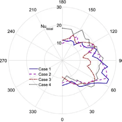
The non-uniform effect of buoyancy on heat transfer can be demonstrated by studying the distributions ofNuloc(local Nusselt number) on the rod wall which are illustrated inFig. 6. For ease of description, the ‘narrow-gap-facing wall’ is used to refer to
0°<h< 30° of rod-wall, and the ‘wide-gap-facing wall’ refer to the region 150°<h< 180°. The main channel covers the range from 45°to 90°. As expected,Nulocvaries significantly from location to location in the forced convection case. The maximum value is located on the wall facing the main channel. Interestingly, Nuloc in the narrow gap is about the same or even higher than that in the wide gap. This is likely due to the existence of the swinging flow structures which greatly enhances the mixing between the fluid in the narrow gap and the main channel. The effect of buoy-ancy onNulocis rather complex. The value ofNulocin the narrow gap generally reduces with the increase of buoyancy in Cases 2 3 & 4, except for the centre region of the narrow gap in Case 4. Here a weak recovery ofNulocis observed. For the locations facing the main channel, the general trend is thatNulocreduces in Cases 2 and 3, but recovers in Case 4. In contrast with the main channel, theNulocis only impaired in the centre of the wide gap in Cases 2; it is greatly enhanced in other cases, especially in Case 4. The dif-ferent responses of heat transfer to buoyancy observed in the var-ious regions are believed to be caused by the non-uniform distribution of buoyancy through modifying the flow structures.
3.2. Buoyancy effects on the regional flow
3.2.1. The mean velocity
The cross-sectional distributions of the axial velocity (W) in the various cases are shown in Fig. 7. As expected, a high-velocity patch is located in the main channel in the forced convection case (Case 1). The velocity decreases as the flow passage becomes nar-rower. The mass flow is re-distributed once the buoyancy force is introduced into the system. The high-velocity patch is moved to the top corner and spreads to the wide gap in Case 2. With the increase of the buoyancy force, this patch also spreads towards the main channel, see Case 3. When the buoyancy force is suffi-ciently high, the velocities in the bottom narrow gap and the cor-ners are greatly accelerated, as demonstrated in Case 4. It is clear that buoyancy plays a great role in the redistribution of the mass flow in the channel.
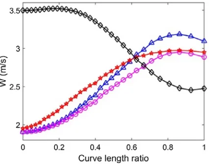
The velocity distributions along ‘P1’, ‘P2’ and ‘P3’ are shown in
[image:5.595.154.450.581.737.2]Fig. 8 to further demonstrate the local flow characteristics and the influence of buoyancy. In general, the velocity profile is signif-icantly different in the different regions. A typical turbulent flow velocity profile is seen along ‘P2’ and ‘P3’, but a parabolic velocity profile is observed along ‘P1’ in Case 1, which implies that the flow is laminar-like in the narrow gap (even though some turbulence is present). Subsequently, the buoyancy influences on flow varies in different regions, which cause the complex buoyancy effect on the local heat transfer rate as described above. The velocity profiles
along ‘P1’ (i.e., in the narrow gap) practically overlap each other in Cases 1, 2 & 3, while the velocity is greatly accelerated in Case 4, which results in a significant advection. It will be shown later, this also leads to a greater turbulence generation. Along ‘P2’, the veloc-ity magnitude and gradient in the near wall region are reduced slightly in Cases 2 & 3 compared to those in Case 1. The mean velocity decreases further in Case 4, but the velocity gradient near the wall increases, which results in a half ‘M-shape’ velocity. The velocity along ‘P3’ (i.e., in the wide gap) is accelerated in Cases 2, 3 & 4 in comparison with that in Case 1. The accelerated flow in the region results in a higher velocity gradient near the wall. How-ever, the change of near wall velocity gradient is non-monotonic as buoyancy is increased.
3.2.2. Turbulence quantities
The contours ofk=U2
b,hw0i=Ubandhu0i=Ubare shown inFigs. 9–
11. The general distribution of turbulence quantities in the current
channel is quite different from that in a uniform channel. It can be seen inFig. 9that there is a high turbulence kinetic energy region located in the vicinity of the narrow gap in Case 1. This is similar to that found in the experimental work by Wu and Trupp[41,42]. This is mostly due to the large flow structures that are present in the region, which was demonstrated in Duan and He[58]. The overall turbulence kinetic energy is reduced in Cases 2 and 3, but it recov-ers with a further increase in buoyancy in Case 4. In addition, the region over which turbulence is strong is much bigger than in the other three cases. The turbulence kinetic energy is also increased in the core region across the whole of the channel in Case 4. The contours of the axial component of turbulent intensity hw0i=U
bshow similar pictures as the turbulence kinetic energy dis-tributions in the various cases, seeFig. 10. The high-value patches are located near the wall and the region close to the narrow gap. In comparison with Case 1, the overall magnitudes ofhw0i=U
[image:6.595.135.445.66.348.2]band the sizes of the high-value patches are reduced in Case 2 and more Fig. 4.Contours of normalized averaged temperaturehTi.
[image:6.595.122.462.380.520.2]strongly in Case 3. When the body force is further increased, the turbulence intensity recovers as seen in Case 4. Furthermore, the value ofhw0i=U
bin the core region is much higher in Case 4 than in other cases. It can be seen inFig. 11, the high-value patches of hu0i=U
b are located in the narrow gap in first three cases, while an additional high-value patch is visible in the wide gap in Case 4. Interestingly, the maximum values of hu0i=Ub in the narrow gap are located away from the wall in all cases. Like the contours ofk=U2
bandhw0i=Ubshown above, the size of the high-value patch in the narrow gap is reduced with the increase of buoyancy force in
the Cases 2 & 3 but recovers in Case 4, although the magnitude in Case 4 is still smaller than that in the forced convection case.
To further understand the buoyancy effects on flow in different regions of the channel, the values ofk=U2bhw0i=Ubandhu0i=Ubalong the predefined lines (‘P1’, ‘P2’ & ‘P3’) are presented inFigs. 12–14. First, it can be seen that the values of all three quantities are very high in the narrow gap, see the profiles on ‘P1’. Different from a typical turbulent flow, the maximum values occur in the centre of the narrow gap. For the forced convection case,hu0i=Ubin the centre of the narrow gap is significantly greater than that of hw0i=U
b. This reflects the presence of the swinging flow structures in that region. Generally speaking, all three turbulence quantities reduce in Cases 2 & 3 but recover in Case 4. It can be argued that the stronger reduction inhw0i=U
bthan inhu0i=Ubin the laminariz-ing cases implies that the buoyancy effect on the local generation of root-mean-square (r.m.s.) values is stronger than its effect on the generation due to the swinging flow structures. It is also inter-esting to know that the recovery ofhw0i=Ubis stronger than that of hu0i=Ubin Case 4.
The turbulent quantities in the main channel (‘P2’) in Case 1 lar-gely show a characteristic of a wall shear flow (Fig. 13). The peaks of the turbulence quantities are located close to the wall. In addi-tion, the effect of the buoyancy on the turbulence in this region is similar to the mixed convection in a pipe. A reduction of the tur-bulent kinetic energy is observed in Cases 2 & 3, while turbulence is regenerated in the region further away from the wall in Case 4 though the turbulence level in the near wall region is still smaller than that of forced convection. It is reasonable to assume that there is an additional mechanism for heat transfer recovery in the region, namely, one associated with the swinging flow. Different from the pipe flow,hu0i=U
bis about 40% ofhw0i=Ubin the near wall region and they are comparable in the core region in Case 1 as a result of the swinging flow. In addition, hu0i=U
b reduces with increase of buoyancy, refer to the results of Cases 2 & 3, buthw0i=U
[image:7.595.63.271.68.276.2]bremains Fig. 6.Local Nusselt number (Nuloc) on the rod wall.
[image:7.595.142.459.453.740.2]about the same in both cases. Furthermore, in Case 4,hu0i=U bin the near wall region starts to recover, whilehw0i=U
bis further reduced.
Fig. 14shows that a typical turbulent kinetic energy distribu-tion is again observed along ‘P3’ in the forced convecdistribu-tion case. The peaks ofk=U2bandhw0i=Ubcan be found in the near wall region and a minimum is located close to the centre of the wide gap. This ‘M’ shape is preserved in Cases 2 & 3 while the profiles are flat-tened in Case 4. The values of k=U2b and hw0i=Ub are increased slightly in Case 2, but rather strongly reduced in Case 3, while a recovery occurs in Case 4. The profile ofhu0i=U
b is different. It is rather flat across the region in Cases 1 & 2, but peaks in the centre of the wide gap in Case 3. Then, in Case 4, the quantity significantly increases, which becomes the major source of the recovery ofk=U2b. Evidently, hw0i=U
b in the vicinity of the wall is much smaller in Case 4 than in Case 1, butk=U2
b in the same region is close to the forced convection value due to the contribution ofhu0i=U
b. It is also worth to note that all these turbulence quantities are lower in Case 2 in comparison with those in Case 1. The buoyancy influence on the large flow structures in the wide gap is likely to be the main reason for the abnormal changes of hu0i=Ub in the buoyancy
influenced cases. As demonstrated in[58], large flow structures in the wide gap are enhanced in Cases 3 and 4 by buoyancy but suppressed in Case 2. This can also explain the impaired heat trans-fer rate in the wide gap centre of Case 2, in spite of increased turbulence.
3.2.3. Production of turbulent kinetic energy
[image:8.595.69.518.66.187.2]There are two sources contributing to the production of turbu-lent kinetic energy in mixed convection. One is the production due to shear stress (huiujiSij) and the other is buoyancy production (bhw0T0ig). The distribution of these two terms along ‘P1’, ‘P2’ & ‘P3’ are presented inFigs. 14–16. Although the velocity profile in the narrow gap in Case 1 demonstrates a laminar-like flow, there are still some production (huiujiSij) which peaks in the near-wall region, refer toFig. 15. Such a shear production decreases as the heat flux increases in the laminarizing cases (Case 2 & 3). The shear production recovers in Case 4 and becomes significantly higher than in Case 1. The buoyancy production peaks (negative in Cases 2 & 3) at the centre of the narrow gap and is likely to be associated with the swinging flow structure. The magnitude of maximum Fig. 8.Reynolds averaged streamwise velocityW(m/s) along lines (a) ‘P1’; (b) ‘P2’; (c) ‘P3’.
Fig. 9.Contours of turbulent kinetic energy (k=U2
[image:8.595.135.449.224.502.2]Fig. 10.Contours of the axial component of turbulence intensity (hw0i=Ub) in different cases.
[image:9.595.144.457.416.701.2]buoyancy production in all cases but Case 4 is negligibly small. In the latter case, the buoyancy production is significant even though it is still smaller than the shear production. The recovery of the shear production and enhanced buoyancy production on ‘P1’ in Case 4 can be one of the reasons for the recovery of heat transfer
at the centreline of the narrow gap, while the heat transfer in the narrow gap region is still overall impaired.
[image:10.595.63.520.63.495.2]Similar to the pipe flow, thehuiujiSijalong ‘P2’ peaks in the near-wall region in Case 1, refer to Fig. 16. The shear production decreases with the increase of buoyancy. Furthermore, the Fig. 12.The distributions ofk=U2
[image:10.595.65.518.65.187.2]b,hw0i=Ubandhu0i=Ubalong ‘P1’.
Fig. 13.The distributions ofk=U2
b,hw0i=Ubandhu0i=Ubalong ‘P2’.
Fig. 14.The distributions ofk=U2 b,hw0i=U
bandu0=Ubalong ‘P3’.
[image:10.595.64.520.374.498.2] [image:10.595.123.464.533.664.2]buoyancy production is negative in the near wall region. The tion of the minima of the buoyancy production is close to the loca-tion of the peak of the shear producloca-tion, but the magnitude is negligible compared to the shear production. The buoyancy pro-duction away from the wall is rather higher in Case 4. The magni-tude of such production is still much smaller than the production due to the shear stress, but since the velocity gradient in the core region is not very strong, the dissipation is not as strong as near the wall. It is likely that such buoyancy production is responsible for the recovery of the turbulence in the main channel of this case. Here the shear production is very low.
The profile ofhuiujiSijalong ‘P3’ shows that the turbulence pro-duction is stronger in Case 2 than in Case 1, which results in a higher turbulence in the wide gap in this case as discussed above, refer toFig. 17. At first sight, this is against our understanding of buoyancy-aided flow where buoyancy should cause a reduction in turbulence. However, the real reason for this increase of produc-tion is the buoyancy induced redistribuproduc-tion of the mean flow (Fig. 7), which causes a significant increase in velocity in the wide gap. The value of huiujiSij decreases in Case 3 as expected, but recovers in Case 4 with location of peak moving towards the wall. The recovery of the shear production occurs near the wall but its magnitude is not very high. There is also some positive buoyancy production in the central region of the gap. The magnitude is not particular high, but as explained above, since the dissipation in the core is weak due to a low velocity gradient, this relatively small buoyancy production may be the main reason for the high turbu-lence in Case 4 in the wide gap.
3.3. Buoyancy effect on the large flow structures: a statistic view
The effects of buoyancy on the instantaneous behaviours can be found in[58]. That article demonstrated that the flow structures
driven by the velocity gradient across the narrow gap cause a strong mixing between the narrow gap and main channel. The mixing factor due to the existence of the flow structures is nega-tively correlated with the buoyancy. Especially, the rotating direc-tion of the vortexes of the flow structures is reversed once the buoyancy is strong enough to reverse the velocity distribution in the region. The discussion in the previous section has demon-strated the significance of the large flow structures on the local heat transfer. In this section, the buoyancy effect on the large swinging flow structures in the narrow gap is studied from a statis-tical view.
First, the velocity distribution from the middle of the narrow gap to the centre of the main channel is illustrated using the veloc-ity profile along ‘ML’, as shown inFig. 18. It is clear that velocity distribution across the region is influenced by buoyancy. The veloc-ity in the centre of the narrow gap in Cases 2 and 3 is about the same as that in Case 1, whereas the flow in the main channel is decelerated somewhat, and as a result, the velocity gradient is reduced. Consequently, the shear production due to the swinging flow structures reduces in Cases 2 & 3. Because the flow around the narrow gap is greatly accelerated in Case 4, the velocity profile in the region is reversed.
The turbulence quantities (k=U2
b,hw0i=Ubandhu0i=Ub) as well as the turbulent heat flux u0T0=ðUbTwallÞ on ‘ML’ are presented in
Fig. 19. Similar to the near wall turbulence, the turbulence kinetic energy reduces in the laminarization cases, recovers strongly in Case 4. As illustrated in the figure, the reduction ofk=U2
bis mostly due to the reduction ofhw0i=U
b andhu0i=Ubin Cases 2 & 3. How-ever, the increase ofhw0i=Ubcontributes much more to the recov-ery ofk=U2
b than hu0i=Ub in Case 4. As the flow structure in the narrow gap is swinging around the centre, the lowerhu0i=U
b indi-cates weaker flow structures in the region. It should also be noticed that the level ofhu0i=U
[image:11.595.132.473.67.199.2]baway from the centre of the narrow gap is Fig. 16.The distributions of shear production (huiujiSij) and the buoyancy production (bhw0T0ig) of the turbulence kinetic energy along ‘P2’.
[image:11.595.131.474.609.739.2]high in Case 4 which reflects the significant increase ofhu0i=U b in the core region of the main channel. The weakened large flow structure in the narrow gap leads to a smaller u0T0=ðU
bTwallÞ in the buoyancy influence case, seeFig. 19, whereas some recover-ing/strengthening ofu0T0=ðU
bTwallÞoccurs in the main channel part in Case 4. In addition, the peaks ink=U2
bandhw0i=Ubmove towards the centre of the narrow gap in Cases 2 & 3 but away from it in Case 4. This indicates the movements of the vortex’s centre of flow structures in the narrow gap. The shift of the location of the vor-texes from the narrow gap towards the main channel in Case 4 leads to a stronger mixing in the main channel which improves local heat transfer.
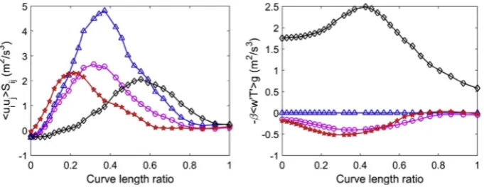
To further understand the contribution of large flow structures to the turbulence in the narrow gap and main channel, the produc-tion of turbulence along ‘ML’ is presented in Fig. 20. Consistent with the turbulence quantities discussed earlier, the maximum shear production decreases with the increase of the buoyancy. Due to the shift of the location of the inflection point of the velocity
4. In addition, the change of the sign of the buoyancy production supports the proposition by Duan and He[58] that the rotation direction of the vortexes of the large flow structures reverses once the buoyancy is sufficiently strong to reverse the velocity profile across the narrow gap.
In summary, it is reasonable to conclude that, in the narrow gap, the large flow structure is an important source of turbulence. The reduced turbulence and shear production along ‘ML’ and the shift of the location of the maximum shear production due to the buoy-ancy support the findings of Duan and He[58], namely, the nega-tive correlation between buoyancy and mixing velocity due to large flow structures, as well as the significantly narrowed flow structures in the recovery case. The heat transfer impairment in the narrow gap of the laminarization cases is mainly due to the weakening of large flow structures. The reason for the low heat transfer rate in this region in Case 4 is more complicated. First, the greatly accelerated flow causes an increase in the local mass flow rate and advection. Secondly, overall turbulence kinetic energy is increased in this region, but this is largely due to the increase ofhw0i=U
[image:12.595.53.266.66.234.2]b; the value ofhu0i=Ub remains relatively low. Subsequently, the mixing remains low. In addition, the mixing between the narrow gap and main channel is greatly impaired due to the shift of the velocity inflection point, the reduced hori-zontal size of the flow structure and mixing velocity, refer to Duan and He[58]. This negative effect overrides the increased advection and local turbulence production in the narrow gap region, resulting in a reduction in heat transfer in the region. However, the Fig. 18.Reynolds averaged streamwise velocityW(m/s) along ‘ML’.
Fig. 19.The distributions ofk=U2 b,hw0i=U
[image:12.595.119.461.483.738.2]relocation of the large flow structures enhances the mixing in the main channel. This explains the recovery of heat transfer at some locations of the main channel (Nuloc around 60° on ‘Rod-Wall’) even though turbulence near the wall continues to decrease. Sim-ilar explanation is applicable to the unexpected effect of buoyancy onNulocin the wide gap. The heat transfer rate is reduced in Case 2 despite that the turbulence is increased in the region. Recovery occurs in Case 3, which becomes more significant in Case 4. The reason for this unusual observation can be associated with the weakened flow structures in Case 2 and enhanced ones in Cases 3 & 4, refer to[58].
4. Conclusions
The complex buoyancy effects on the mixed convection heat transfer of the flow at a Reynolds number of 5270 in a triangular-array rod-bundle-like channel have been investigated. The general behaviour of the predicted flow domain (including large flow structures and turbulence field) in the forced convection is line with the experimental observation of Wu and Trupp[41,42]. The predicted averaged Nusselt number of the forced convection in this flow passage is similar to that of a pipe flow and the eccentric annulus with high eccentricity.
Thanks to the enhanced mixing due to the large flow structures in the narrow gap, the local heat transfer rate in that region is unexpectedly high. The general trend of buoyancy effect on the heat transfer in the current channel is similar to that in a pipe. Heat transfer deterioration occurs in the so-called laminarizing regime, while heat transfer is improved in the recovery regime. However, heat transfer impairment occurs earlier (i.e., at a relative weaker buoyancy) in the current channel, though the maximum impair-ment is less significant than in the pipe flow. Furthermore, the recovery in the considered flow is stronger than in the pipe flow. The buoyancy effect on local heat transfer shows a great complex-ity. In general, heat transfer rate in the narrow gap is negatively correlated to the buoyancy parameterBo⁄, whereas the effect of buoyancy in the main channel and the wide gap follows the typical trend. Interestingly, the buoyancy impairment in the wide gap is much weaker than in the main channel and the recovery is earlier and stronger.
A number of factors are responsible for the non-uniform buoy-ancy effect on the local heat transfer, namely, the regional varia-tions of buoyancy effect, the redistribution of mass flow and the modified behaviour of the large flow structures due to the buoy-ancy force. In forced convection, the parabolic velocity profile observed in the centre of the narrow gap suggests that the flow in this region is laminar-like, whereas typical turbulent velocity profiles are observed in the main channel and the wide gap. Thus the regional flow responds to the non-uniform buoyancy varies
largely around the channel. The flow in the gaps (narrow/wide) is more likely to be accelerated due to buoyancy, which results in a deceleration in flow in the main channel. Thanks to this redis-tribution of mass flow in the channel, some ‘unusual’ turbulence response to the buoyancy occurs. In addition, the redistribution of the mass flow causes the behaviour of large flow structures also change, which leads to more complicity to the buoyancy influences on the local heat transfer. For instance, the overallNulocreduces as buoyancy increases, despite the enhancement of the advection and relatively high turbulence in the near wall region of the narrow gap. The weakening of the swinging flow structures in the region, such as the reduced horizontal size of the large flow structures and mixing velocity due to them, is likely to be the main cause. Furthermore, the vortexes of the swing flow structures may move away from the narrow gap in the cases where the heat flux is strong, such as that in the recovery case (Case 4). Consequently, the heat transfer effectiveness in the region remains low, but the mixing in the regions away from the narrow gap is however increased. The buoyancy influence on the large flow structures in the wide gap also influences the local heat transfer.
Overall, the three factors mentioned above, namely, the mass flow redistribution, buoyancy influence on local turbulence, and the behaviour of large flow structures, together make the influ-ences of buoyancy on the flow in flow channel concerned very complicated. Similar to the effect of turbulence, the weakening of the flow structures in the buoyancy-aided flow with a small Bo⁄
worsens the heat transfer deterioration, whereas the enhancement of the structures in a flow with a largerBo⁄either mitigates the heat transfer impairment or improves the heat transfer recovery.
Conflict of interest
The authors declared that there is no conflict of interest.
Acknowledgements
The authors would like to acknowledge the financial support provided by EDF Energy through Contract 40326718 as well as the support of the EPSRC through UK Turbulence Consortium (grant no. EP/L000261/1), which provides access to the facilities of the UK national supercomputer ARCHER.
References
[1]B.S. Petukhov, A.F. Polyakov, Heat Transfer in Turbulent Mixed Convection, Hemisphere Publishing Corporation, New York, 1988.
[2]J.D. Jackson, M.A. Cotton, B.P. Axcell, Studies of mixed convection in vertical tubes, Int. J. Heat Fluid Flow 10 (1989) 2–15.
[image:13.595.132.473.66.198.2][3] J.D. Jackson, Studies of buoyancy-influenced turbulent flow and heat transfer in vertical passages, in: Keynote Lecture at 13th International Heat Transfer Conference, IHTC13, Sydney, Australia, 13–18 August 2006.
Mass Transfer 30 (1987) 165–174.
[10]M.A. Cotton, Theoretical Studies of Mixed Convection in Vertical Tubes Ph.D. Thesis, The University of Manchester, 1987.
[11]M.A. Cotton, J.D. Jackson, Vertical tube air flow in the turbulent mixed convection regime calculated using a low-Reynolds-number k-emodel, Int. J. Heat Mass Transfer 33 (1990) 275–286.
[12]A. Behzadmehr, N. Galanis, A. Laneville, Low Reynolds number mixed convection in vertical tubes with uniform wall heat flux, Int. J. Heat Mass Transfer 46 (2003) 4823–4833.
[13] J. Wang, J. Li, S. He, J.D. Jackson, Computational simulations of buoyancy-influenced turbulent flow and heat transfer in a vertical plane passage, Proc. Inst. Mech. Eng. Part C: J. Mech. Eng. Sci. 218 (2004).
[14]W.S. Kim, S. He, J.D. Jackson, Assessment by comparison with DNS data of turbulence models used in simulations of mixed convection, Int. J. Heat Mass Transfer 51 (2008) 1293–1312.
[15]B.E. Launder, B.I. Sharma, Application of the energy-dissipation model of turbulence to the calculation of flow near a spinning disc, Lett. Heat Mass Transfer 1 (1974) 131–137.
[16]K.Y. Chien, Predictions of channel and boundary-layer flows with a low-Reynolds number turbulence model, AIAA J. 20 (1982) 33–38.
[17]C.K.G. Lam, K. Bremhorst, A modified form of the k–e model for predicting wall turbulence, Trans. ASME 103 (1981) 456–460.
[18]K. Abe, T. Kondoh, Y. Nagano, A new turbulence model for predicting fluid flow and heat transfer in separating and reattaching flows—I. Flow field calculations, Int. J. Heat Mass Transfer 37 (1994) 139–151.
[19]D.C. Wilcox, Reassessment of the scale determining equation for advanced turbulence models, AIAA J. 26 (1988) 1299–1310.
[20]Z. Yang, T.H. Shih, New time scale based k–e model for near-wall turbulence, AIAA J. 31 (1993) 1191–1198.
[21]H.K. Myoung, N. Kasagi, A new approach to the improvement of k– e turbulence model for wall bounded shear flows, JSME Int. J. 33 (1990) 63–72. [22] C.B. Hwang, C.A. Lin, Low-Reynolds number modelling of transpired flows, in:
2nd EF Conference in Turbulent Heat Transfer, Manchester, UK, 1998. [23]M. Behnia, S. Parneix, P.A. Durbin, Prediction of heat transfer in an
axisymmetric turbulent jet impinging on a flat plate, Int. J. Heat Mass Transfer 41 (1998) 1845–1855.
[24]M.A. Cotton, P.J. Kirwin, A variant of the low-Reynolds-number two-equation turbulence model applied to variable property mixed convection flows, Int. J. Heat Fluid Flow 16 (1995) 486–492.
[25]N. Kasagi, M. Nishimura, Direct numerical simulation of combined forced and natural turbulent convection in a vertical plane channel, Int. J. Heat Fluid Flow 18 (1997) 88–99.
[26]J. You, J.Y. Yoo, H. Choi, Direct numerical simulation of heated vertical air flows in fully developed turbulent mixed convection, Int. J. Heat Mass Transfer 46 (2003) 1613–1627.
[27]J.S. Lee, X. Xu, R.H. Pletcher, Large eddy simulation of heated vertical annular pipe flow in fully developed turbulent mixed convection, Int. J. Heat Mass Transfer 47 (2004) 437–446.
[28] A. Keshmiri, M.a. Cotton, Y. Addad, D. Laurence, Turbulence models and large eddy simulations applied to ascending mixed convection flows, Flow Turbul. Combust. 89 (2012) 407–434.
[29]A.K. Chauhan, B.V.S.S.S. Prasad, B.S.V. Patnaik, Numerical simulation of flow through an eccentric annulus with heat transfer, Int. J. Numer. Methods Heat Fluid Flow 24 (2014) 1864–1887.
[30]P. Forooghi, I.A. Abdi, M. Dahari, K. Hooman, Buoyancy induced heat transfer deterioration in vertical concentric and eccentric annuli, Int. J. Heat Mass Transfer 81 (2015) 222–233.
[31]J.D. Hooper, K. Rehme, Large-scale structural effects in developed turbulent flow through closely-spaced rod arrays, J. Fluid Mech. 145 (1984) 305–337. [32]S.V. Moller, On phenomena of turbulent flow through rod bundles, Exp. Therm.
Fluid Sci. 4 (1991) 25–35.
lattice rod-bundle, Nucl. Eng. Des. 241 (2011) 4621–4632.
[40]Y. Duan, S. He, P. Ganesan, J. Gotts, Analysis of the horizontal flow in the advanced gas-cooled reactor, Nucl. Eng. Des. 272 (2014) 53–64.
[41]X. Wu, A.C. Trupp, Experimental study on the unusual turbulence intensity distributions in rod-to-wall gap regions, Exp. Therm. Fluid Sci. 6 (1993) 360– 370.
[42]X. Wu, A.C. Trupp, Spectral measurements and mixing correlation in simulated rod bundle subchannels, Int. J. Heat Mass Transfer 37 (1994) 1277–1281. [43]M.S. Guellouz, S. Tavoularis, The structure of turbulent flow in a rectangular
channel containing a cylindrical rod – part 1: Reynolds-averaged measurements, Exp. Therm. Fluid Sci. 23 (2000) 59–73.
[44]M.S. Guellouz, S. Tavoularis, The structure of turbulent flow in a rectangular channel containing a cylindrical rod – part 2: phase-averaged measurements, Exp. Therm. Fluid Sci. 23 (2000) 75–91.
[45]E. Piot, S. Tavoularis, Gap instability of laminar flows in eccentric annular channels, Nucl. Eng. Des. 241 (2011) (Feb. 2011) 4615–4620.
[46]G.H. Choueiri, S. Tavoularis, Experimental investigation of flow development and gap vortex street in an eccentric annular channel. Part 1. Overview of the flow structure, J. Fluid Mech. 752 (2014) 521–542.
[47]L. Meyer, K. Rehme, Large-scale turbulence phenomena compound rectangular channels, Exp. Therm. Fluid Sci. 8 (1994) 286–304.
[48] L. Mayer, K. Rehme, Periodic vortices in flow through channels with longitudinal slots or fins, in: 10th Symposium on Turbulent Shear Flows, The Pennsylvania State University, USA, 14–16 August 1995.
[49]D. Home, M.F. Lightstone, Numerical investigation of quasi-periodic flow and vortex structure in a twin rectangular subchannel geometry using detached eddy simulation, Nucl. Eng. Des. 270 (2014) 1–20.
[50]A. Gosset, S. Tavoularis, Laminar flow instability in a rectangular channel with a cylindrical core, Phys. Fluids 18 (2006) 044108.
[51]L. Meyer, From discovery to recognition of periodic large scale vortices in rod bundles as source of natural mixing between subchannels—a review, Nucl. Eng. Des. 240 (2010) 1575–1588.
[52]E. Merzari, H. Ninokata, Anisotropic turbulence and coherent structures in eccentric annular channels, Flow Turbul. Combust. 82 (2008) 93–120. [53]E. Merzari, H. Ninokata, Development of an LES methodology for complex
geometries, Nucl. Eng. Technol. 41 (2009) 893–906.
[54]D. Chang, S. Tavoularis, Numerical simulations of developing flow and vortex street in a rectangular channel with a cylindrical core, Nucl. Eng. Des. 243 (2012) 176–199.
[55]G.H. Choueiri, S. Tavoularis, An experimental study of natural convection in vertical, open-ended, concentric, and eccentric annular channels, J. Heat Transfer 133 (12) (2011) 122503.
[56]L. Maudou, G.H. Choueiri, S. Tavoularis, An experimental study of mixed convection in vertical, open-ended, concentric and eccentric annular channels, J. Heat Transfer 135 (7) (2013) 072502.
[57]N. Kline, S. Tavoularis, An experimental study of forced heat convection in concentric and eccentric annular channels, J. Heat Transfer 138 (1) (2016) 012502.
[58]Y. Duan, S. He, Large eddy simulation of a buoyancy aided flow in a non-uniform channel – Buoyancy effects on large flow structures, Nucl. Eng. Des. 312 (2017) 191–204.
[59]F. Nicoud, F. Ducros, Subgrid-scale stress modelling based on the square of the velocity gradient tensor, Flow Turbul. Combust. 62 (1999) 183–200. [60]S.V. Patankar, C.H. Liu, E.M. Sparrow, Fully developed flow and heat transfer in
ducts having streamwise-periodic variations of cross-sectional area, ASME J. Heat Transfer 99 (1977) 180–186.
[61] A. Fluent, Theory Guide: ANSYS Inc, 2009.
[62]B. Celik, Z.N. Cehreli, I. Yavuz, Index of resolution quality for large eddy simulations, J. Fluids Eng. 127 (2005) 949–958.