Seismic body wave attenuation tomography beneath the Australasian region

(1)

Seismic Body Wave

Attenuation Tomography

beneath the Australasian region

Agus Abdulah

A thesis submitted for the degree of

Doctor of Philosophy

of The Australian National University

(2)

Except where otherwise indicated in the

text, the research described in this thesis is

my own original work.

Agus Abdulah

(3)

Acknowledgements

This thesis has benefited from the assistance of a number of people. First, and

foremost, I owe the greatest intellectual and personal debt to Professor Brian L.N.

Kennett, my supervisor. Professor Kennett provided excellent guidance and support

throughout my doctoral research and his detailed comments on my thesis helped me to

improve it in every aspect. He gave me a detailed advice as to how to design and

develop my research. I received inestimable knowledge from Brian.

I would like to express my gratitude to my thesis advisors: Professor Ian

Jackson, Dr. Anya M. Reading, Dr. Malcolm Sambridge and Dr. Nick Rawlinson for

their invaluable guidance and generosity with time and energy. Discussion with

Professor Ian Jackson on the attenuation and the frequency dependence of attenuation

from the laboratory measurement point of view was very useful. Dr. Anya M. Reading

introduced me to basic seismology and seismic tomography inversion. Assistance and

permission from Dr. Nick Rawlinson and Dr. Malcolm Sambridge to use their Fast

Marching Method code was really valuable on the development of the 3-D ray tracing

presented in Chapter 5.

I have benefited from discussion with Professor Douglas A. Wiens and Dr. Eric

Debayle during their visit to the ANU as well as discussion with Dr. Irina Artemieva in

the European Geosciences Union meeting in Vienna 2006. I thank to Dr. Teddy Surya

Gunawan from School of Electrical Engineering and Telecommunications, University

of New South Wales who introduced me the Multitaper Method in Digital Signal

(4)

I am grateful to Dr. Cvetan Sinadinovski for his kind support and help to do P -Wave Tomography of Northwestern Australia which is presented in Appendix A. Also

for his suggestion to introduce the Root-mean Square (equation A.1) in this

tomographic inversion. An incredible support from Armando Arcidiaco to provide

seismic data was highly appreciated.

My special thanks are due to staff at Institut Teknologi Bandung, particularly

Prof. Djoko Santoso, Prof Tachyuddin Taib (alm), Dr. Sri Widiyantoro, Dr. Teuku Abdullah Sanny, Dr. Sigit Sukmono, Dr. Darharta Dahrin and many other staff for their

support and encouragement to study at the Australian National University (ANU).

This work has been supported through an ANU (Australian National University)

PhD Scholarship and ARC (Australian Research Council) Discovery Grant DP0342618.

I would like to express my sincerest gratitude to the ANU and the ARC Grant

program-the Australian Government.

Heartfelt thanks go to my beloved wife, Della Temenggung, for her support,

excellent understanding and great encouragement, and my children: Azzam and Aaqil

who missed a lot of my company especially after sunset which was my prime time to do

computer programming and seismic data measurements. I wish to express my sincerest

appreciation to members of my family: my parents (alm), Mami, Papi, kang Wawan, ceu Apong, Kiyai Fanny, Takunan, Ses Eza, Yani, Sony and many others who

understood and tolerated me going overseas to undertake my PhD research.

A long period of study would not have been possible without warm and friendly

environment. I greatly appreciate the kindness of all Research School of Earth Sciences

staff and students, in particular my roommates: Erdinç Saygin, Ima Itikarai and Andreas

Fichtner. Finally, I am very grateful to all Indonesian community in Australia,

particularly colleagues and friends at the Indonesian Embassy, KMI-ANZ, PPIA, TPA

CERIA, ANUMA, PERMATA and BBC (especially Dodi Darmadi).

Agus Abdulah

(5)

Abstract

Geological features in the lithosphere and the upper mantle beneath the Australasian region have been studied through the analysis of thousands of seismograms recorded by portable seismic stations installed across Australia. The seismic studies were designed to extract information on 1-D and 3-D physical properties such as compressional and shear seismic wavespeeds, seismic anisotropy and attenuation.

Previous seismic studies have mostly been directed to constraining the seismic wavespeed distribution. However, knowledge of the pattern of seismic attenuation is still limited. Seismic attenuation is important as it is sensitive to different physical properties than the wavespeed. Attenuation links to geological features of the earth such as lithology and is frequently used to probe the temperature distribution.

This study uses different classes of information to extract the seismic attenuation distribution beneath the Australasian region by exploiting thousands of seismograms recorded across Australia from 1993 to 2006. A tomographic technique is used to invert differential attenuations of phases on and between these seismograms, which were measured through a spectral ratio method.

The differential attenuation between S and P seismic waves

( )

* SP

t

Δ , between S

and S

( )

* SS

t

Δ , and between P and P

( )

* PP

t

Δ for nearly 6500 event-station pairs refracted back from the mantle have been used to produce 3D images of the attenuation of shear and compressional waves. The values of the differential attenuation are estimated in each case using a spectral ratio method exploiting the Multitaper technique. The

(8)

Abstract iv

frequency band is limited to 0.10 and 1.00Hz with the assumption that attenuation is nearly independent of frequency. This assumption is supported by the linear behavior of the logarithmic spectral ratio as a function of frequency for most seismograms.

The attenuation images depend on knowledge of the propagation paths of the seismic waves, and so a first inversion was made for the P and S wave travel times picked from the same set of seismograms to produce seismic wavespeed images. The use of waves refracted back from the upper mantle leads to some vertical smearing since many of the paths cross the uppermost mantle at steep angles. However the major features of seismic wave speeds and attenuation beneath the Australasian can be reliably delineated down to 320 km depth.

The seismic wavespeeds and attenuation images are produced by two tomographic inversion approaches:

(i) The kernel matrix of the inversion is built by using 1-D ray tracing in 1-D initial models (ak135 seismic speed model and 1-D attenuation model from previous attenuation study).

(ii)The kernel matrix is improved by introducing 3-D initial models derived from surface wave tomography for Australasian region. The Fast Marching Method is used as a powerful algorithm to trace seismic ray paths in this 3-D models.

(9)

Abstract v

characterized by low attenuation for both compressional and shear waves with

Qp=1600-3000; Qs=800-1250, while the upper mantle beneath displays high attenuation i.e. Qp=230-250; Qs=120-140.

Frequency dependence of attenuation beneath the Australasian region is also observed by measuring the differential attenuation between S and P seismic waves

( )

*

SP

t

Δ in a wider frequency band (up to 2.5 Hz). For this purpose, the broad frequency band is divided into four sub frequency bands by using a Golden section division (0.10-1.00 Hz, 0.50-1.50Hz, (0.10-1.00-2.00Hz and 1.50-2.5Hz). Then by using the assumption of a simple power law dependence frequency, the

( )

*

SP

t

Δ from each sub frequency band are used to produce frequency dependence parameter (γ) paths. The

( )

*

SP

t

Δ from each sub- frequency band are also inverted to produce tomographic images of seismic attenuation. Using the same assumption, the tomographic images of frequency dependence of attenuation beneath Australasian region is presented.

The frequency dependence of the paths (γ) covering eastern part of Australia and the Coral Sea area shows larger γ so that the frequency dependence in those areas is relatively stronger. In the north-west part of the Australian continent shows a mixture of paths with small and larger γ suggesting complex frequency dependence. These features are also supported by the tomographic images of frequency dependence of attenuation beneath the Australasian region. The frequency dependence of attenuations (exponent γ) increases with frequency with 0.1 < γ < 0.3 at 35-120km depth interval; 0.02 < γ < 0.21 at 120-220km and 0.0006 < γ < 0.02 at 220-320km for frequency 1.00 – 2.00Hz.

(10)

Chapter 1

Introduction

1.1 Background

The strategic position of the Australian continent between the seismicity belt

which extends from Indonesia to New Zealand through Tonga-Fiji and the mid-ocean

ridge to the south of the continent provides a wealth of events at suitable distances to be

used as probes into the seismic structure of the upper mantle. The extensive

deployments of portable broadband seismic stations across the Australian Continent and

Tasmania since 1993 offer robust seismological data, with over 120 portable stations

that provide a relatively dense coverage at distances from 5° to 45°.

Over the last two decades, a wide range of studies have been used to gain

information on 1-D and 3-D structure in the mantle that exploits different aspects of

seismograms. Studies on seismic tomography which use thousands of seismic travel

times picked from high quality body wave seismograms or use the seismic waveform of

large amplitude surface waves in the later part of the seismogram that travel nearly

horizontally, have been conducted and successfully to delineate the major features of

the geological structure beneath the Australian Continent.

(11)

Chapter 1 - Introduction 2

Seismic travel time tomography for the Australian region was pioneered by

Widiyantoro & van der Hilst [1996] who produced tomographic images in a zone

covering the southern Philippines, Malaysia, Indonesia, Papua New Guinea and

northern Australia. Subsequently, Gorbatov and Kennett [2001] have implemented the

travel time tomographic inversion with a parameterization that has smaller cells near the

earth’s surface and larger cells at the depth.

Efforts in exploring the features of geological structure beneath the Australian

Continent and surrounding regions have exploited surface wave tomography with the

abundance of seismic data recorded by temporary broadband seismometers which have

been deployed in a numerous number of projects conducted by Research School of

Earth Sciences, the Australian National University, such as: SKIPPY

[continent-wide,1993-1996], KIMBA [Kimberley Block, 1997,1998], QUOLL [southeast

Australia, 1999], WACRATON [Western Australia, 2000-2001, 2002-2003], TIGGER

[Tasmania, 2001-2002], TASMAL experiment [Gulf of Carpentaria to the southern

Australia, 2003-] and LINKAGE [Northwestern Australia, 2006-2007].

Zielhuis and van der Hilst [1996] implemented the “Partitioned Waveform

Inversion” (PWI) for surface wave tomography, which has two stages of analysis. The

first step generates a shear wavespeed model for each path and the second combines the

path dependent information in to a 3-D model. A three-stage inversion technique for

surface wave tomography has also been applied to the Australian region by Yoshizawa

and Kennett [2004]. In the first stage, path-specific one-dimensional (1-D) shear

velocity profiles are derived from multimode waveform inversion to provide dispersion

information. The information from all paths is then combined to produce multimode

phase speed maps as a function of frequency. In the second stage, the 2-D phase speed

maps are updated by including ray tracing and finite frequency effects through the

influence zone around the surface wave paths over which the phase is coherent. During

the third stage, the 3-D shear wave speed distribution is reconstructed from the set of

(12)

method has been improved by the development of two new techniques [Fishwick,

2005]: multiple starting models are used in the waveform inversion procedure and

introducing a multi-scale component, where the final model is damped towards the large

scale features of the data rather than a global reference model. These new techniques

have been implemented for seismic data from all Australian National University

temporary deployments, and additional data from permanent stations and a temporary

deployment in New Zealand.

Studies on seismic attenuation of the Australasian region were initiated by

Gudmundsson et al. [1994]. They used the spectral ratio between S and P windows for the analysis of 22 seismograms from the WRA broadband instrument and a further four

from portable broadband instruments deployed near Warramunga.

A more recent study of attenuation in the Australian region was carried out by

Cheng [2000]. He studied Australian attenuation structure by estimating the spectral

ratio between P and S waves for nearly 2000 three-component seismograms from SKIPPY project [1993-1996]. The spectra of the P, SV, and SH waves and their accompanying noise were estimated by using Fast Fourier Transform of a single real

function. The differential attenuation of each ray path was then measured by estimating

the slope of spectral ratio of S to P waves. The differential attenuation data were organized into azimuthal corridors and inverted by using the Neighbourhood Algorithm

(NA) to produce a set of 1-D Q profiles. A 3-D Q model at fixed frequency was then constructed by combining these 1-D Q profiles weighted by ray density. The seismic studies in Australasian region, mentioned above, are explained in more detail in Chapter

3.

In this work, thousands of seismograms from previous and recent projects (from

1993 to 2006) are used to produce seismic wavespeeds and attenuation images beneath

the Australasian region using a tomographic technique. Differential attenuation together

(13)

between the picked P and S waves travel times and the results for a reference model. Attenuation images are constructed by utilizing the seismic wavespeeds and the

differential attenuation information. The attenuation measurement methods and

attenuation inversion procedures used in this study are explained in detail in Chapter 2,

4 and 5. The resulting tomographic images are used to improve the understanding in

the interpretation of complex structure and the temperature distribution beneath the

Australian continent and its surrounding regions.

1.2 Thesis Structure

Chapter 2 Attenuation Theory and Measurements

In this chapter, the basic concept of the attenuation process at the microscopic

scale is presented. Attenuation measurements from various laboratory experiments are

discussed and used as a benchmark for understanding the attenuation principles in

seismology. Furthermore, attenuation measurement techniques particularly the

techniques which are used in this study and their implementation for several Australian

seismic datasets are also demonstrated.

Chapter 3 Australasian Setting and Previous Seismic Studies of Australia

The geological and tectonic features of the Australian continent and surrounding

regions are outlined. Previous seismic studies of the Australasian region are discussed in

more detail, with emphasis on probing of the lithospheric and upper mantle structure

particularly from surface wave and attenuation studies.

Chapter 4 Seismic Speeds and Attenuation Tomography-Part I

The main focus of this chapter is the production of seismic wavespeed and

attenuation images in the lithosphere and the upper mantle beneath the Australasian

region. The images are produced by a tomographic technique in which the seismic ray

(14)

incorporated in the tomography are discussed. Also, details of the tomography

procedure, checkerboard tests, model parameterization and the system of equations are

outlined.

Chapter 5 Seismic Speeds and Attenuation Tomography-Part II

The seismic wavespeed and attenuation images beneath the Australasian are

improved by introducing 3-D ray tracing in 3-D initial models rather than a 1-D

reference model. The initial models used in this study represent geological features of

the Australasian region derived from surface wave tomography. In this way, the starting

point should lie close to the desired solution. Besides the improvement of estimates of

shear attenuations, the pattern of compressional attenuation is also presented.

Chapter 6 Frequency Dependence of Attenuation beneath Australasian

Work on the frequency dependence of attenuation beneath the Australasian

region is presented in this Chapter. The frequency dependence of the attenuation

measurement method, the frequency dependence of the properties of the propagation

paths and frequency dependence tomography are also revealed.

Chapter 7 Discussion

The models derived in the previous chapters are discussed in Chapter 7. An

overview of comparison with previous wavespeeds and attenuation studies is provided.

Further, a discussion of the correlation between attenuation, seismic speed and

temperature beneath the Australasian region along with the study of the frequency

dependence of attenuation and attenuation anisotropy is given.

Appendix

(15)

outlined in Appendix B. The spectral theory of the multi taper method used in chapter 2

is also described in Appendix C. Digital version of this thesis and computer program for

attenuation measurement are enclosed in a compact disc with the instruction is shown in

(16)

Chapter 2

Attenuation Theory and Measurements

2.1 Attenuation Theory

If a seismic wave passes through a material that is not perfectly elastic, it loses energy to the material and the amplitude of the wave gradually diminishes. This amplitude decrease is called attenuation, and its due to anelastic damping of the vibration of the particles in the material [Lowrie, 2004]. The attenuation during the passage of a wave through the Earth’s interior is usually considered to be a combination of two mechanisms, intrinsic absorption and scattering loss due to distributed heterogeneities. The most important evidence for the existence of small-scale random heterogeneities is the existence of "coda" such as the tail portion of the seismograms of local earthquakes [Sato et al., 1998], or the extended wavetrains following the onset of the P and S waves for many Indonesian earthquake recorded in northern Australia. Thus measurements of the attenuation of direct seismic waves need to be carefully considered to see whether total or intrinsic attenuation is important.

The explanation of attenuation due to intrinsic absorption mechanisms can be found in papers reviewed by Knopoff [1964], Jackson and Anderson [1970], Mavko and Nur [1979] and Dziewonski [1979]. Several proposed mechanisms are based on the

(17)

Chapter 2 - Attenuation Theory and Measurements 8

observation that crustal rocks have microscopic cracks and pores which may contain fluids. Intrinsic absorption mechanisms are proposed through frictional sliding on dry surfaces of thin cracks [Walsh, 1966], viscous dissipation in a zone of partially molten rock such as the low velocity or high attenuation zone beneath the lithosphere [Nur, 1971], the effect of partial saturation of cracks on absorption: fluid movement within cracks is enhanced by the presence of gas bubbles [Mavko and Nur, 1979]. An increase of QS−1 with increasing content of volatile in dry rocks revealed by Tittmann et al.,

[1980]. They found that the increase was due to an interaction between an adsorbed water film on the solid surfaces by thermally activated motions. The scattering loss mechanism due to heterogeneities distributed in the earth also causes attenuation [Aki, 1980]. Scattering loss mechanisms caused by distributed crack and cavities have been studied by Matsunami [1990] and Kawahara and Yamashita [1992].

The Quantity of the rate of energy dissipation at frequency ω is provided by the loss factor Q-1(ω), which is defined as the ratio of the energy loss in a circle ∆E(ω) to the elastic energy stored in the oscillation E0 [Kennett, 2001]:

( )

ω

( )

ω

(

π 0

( )

ω

)

1

2 E E

Q− =−Δ _(2.1)

E0 is thesum of the strain and kinetic energy calculated using the instantaneous elastic

moduli, and the energy dissipation ∆E arises from the imaginary part of the elastic moduli. For purely dilatational disturbances

( )

{

1

( )

}

0 1

Im κ ω κ ω

κ− =−

Q (2.2)

and for purely deviatoric effects

( )

{

1

( )

}

0

1 _ω _Im _μ _ω _μ

μ− =−

Q (2.3)

For the earth it appears that loss in pure dilatation is much less significant than loss in shear, and so −1 _<< −1 [Kennett, 2001].

μ

κ Q

Q

The condition of causality leads to relations between dissipation and the frequency dependence of seismic properties so that the real part of μ₁

( )

ω can be written in terms of the loss factor with frequency,

( )

{

}

_∫

∞ −

( )

− ′ ′ ′ ′ − =

0 2 2

1 0 1 2 Re ω ω ω ω ω π μ ω

(18)

where P denotes the Cauchy principal value.

Because of the difficulties in isolating all factors which effect amplitude of a recorded seismic wave, the distribution of the loss factor in the earth is still imperfectly known [Kennett, 2001]. Based on the previous studies on the earth attenuation, it is suggested that the loss factor in the crust is moderate ( ~0.004) with an increase in the uppermost mantle ( ~0.01) and decrease to crustal values, or lower, in the mantle below 1000km. Over the frequency band 0.001-1Hz the intrinsic loss factor appears to be approximately constant [Kennett, 2001].

1 − μ Q 1 − μ Q 1 − μ Q 1 − μ Q

2.2 Laboratory Measurement of Attenuation

Laboratory measurements have been conducted for many years in order to provide a better interpretation of the characteristics of seismic attenuation and dispersion in the earth. To achieve this objective, the measurements are carried out on synthetic materials such as Fo90 Olivine, CaTiO3 Perovskite polycrystals that have

physical properties similar to the real material i.e. formational high temperature and pressure, partially molten, grain size, etc.

Relevant laboratory experiments on seismic attenuation have extensively carried out by RSES, ANU such as a study on Titanate Perovskite CaTiO3 and SrTiO3 at high

temperature [Webb et al., 1999]. They revealed that both of these perovskites display viscoelastic behaviour in the seismic frequency regime; with the temperature of onset of this frequency-dependent behaviour being grainsize-dependent. Also they observed that the rheology of fine-grained SrTiO3 and CaTiO3 perovskites to 5 mm grainsize shows

that a ~20% dispersion in wavespeed is expected for the period range 1–1000 s, with dissipation (Q-1) ~10-2 for 1 s period waves at1300ºC.

The effect of grain size and partial melting on seismic attenuation can be found in the experiment of Jackson et al. [2002] and Faul et al. [2003]. They examine specimens of fine-grained polycrystalline of Fo90 olivine either melt-free or containing

(19)

methods are used to measure the shear modulus and associated strain energy dissipation Q-1 at high temperatures and seismic frequencies. The result suggest that for the nominally melt-free material (containing << 0.1 vol. % melt) a strain-energy absorption band is observed within which Q-1 varies consistently and monotonically with frequency (0.01-1 Hz), temperature (1270-1570 K) and grainsize (3-23 μm). However, at the temperature of 1470 K that represents the upper mantle condition, the value of Q-1 ranges between 0.009 at 10 s period and 10 mm grainsize and 0.034 at 100 s period and 1 mm grainsize. Furthermore, Faul et al. [2003] explored the influence of a small basaltic melt fraction (0.004-0.037) on the seismic properties of fine-grained synthetic polycrystals of Fo90 olivine with torsional forced oscillation/microcreep

methods. They inferred that levels of attenuation for melt-free material are generally consistent with those observed seismologically suggesting that the same grain-boundary diffusional processes thought to dominate the behavior of the fine-grained materials tested in the laboratory might also account for much of the wave speed variability and attenuation in the mantle. Meanwhile, for melt-bearing olivine, the extrapolated attenuation is generally somewhat higher than the highest seismologically measured attenuation. The progress report by Jackson [2000] indicates that dissipation and associated shear modulus dispersion for low-carbon iron alloys and Fo90 Olivine,

CaTiO3 Perovskite polycrystals both increase monotonically with increasing

temperature and decreasing frequency. The extent of the departure from elastic behavior in these generally fine-grained materials appears to be sensitive to both grain size and impurity content.

The effect of temperature on seismic attenuation is also revealed by several laboratory measurements [Gribb and Cooper, 1998]. They observed the high-temperature (1200-1285 °C) torsional dynamic attenuation (10 -10−3 0 _{Hz) and}

unidirectional creep behavior of a fine, uniform grain sized (d≈3μ m) olivine (~Fo92)

aggregate. The attenuation behavior displayed a band in QG−1 that is moderately

(20)

correlation between attenuation and temperature, Jackson [1993] showed that at seismic frequencies attenuation, Q-1, in the mantle rocks at subsoliditus temperatures follows the Arrhenius law and an exponentially dependence in inverse temperature 1/T:

(

E RT

)

A

Q−1 ₌ _ταexp ₋_α */ _(2.5) where _E*_{is the activation energy,}_R_{is the gas constant,}_τ_{is the oscillation period,}_A_is

a scaling constant and the exponent α is approximately 0.15-0.30 as determined from seismic studies and laboratory measurements on the upper mantle rocks.

In separate experiment, Tan et al. [1997] examined shear wave dispersion and attenuation in fine-grained synthetic olivine aggregates using low-frequency torsional forced oscillation tests. The sample has a uniform grainsize of about 50μm, <0.1 vol.% of melt and minor amount of hydroxyl (~100ppm). The tests were conducted under 200MPa hydrostatic pressure, low oscillation frequencies (0.01-1 Hz) and within the linear regime of strain (amplitude < 5x10-5). The sample was first heated at 1300ºC, and subsequently measured at a series of lower temperatures. The result at 1300ºC showed that the shear modulus G is relatively low and strongly frequency dependent and the attenuation Q-1 is high (G ~ 33 GPa, Q-1 ~ 0.14 for 1 Hz). Q-1 varies with temperature and frequency as _Q− ₌ _A

[

_ω_eE _RT

]

−n

0

1 _{with the activation energy for the}

relaxation rate E =420±30 kJ/mol and exponentn=0.31±0.02.

2.3 Attenuation Measurements

Seismic attenuation affects both the amplitude and phase of seismic waves. Algorithms to measure attenuation are divided into those that use amplitude information, or phase information and those that use a combination of both. In this research, a spectral ratio method which uses amplitude information is used to estimate differential attenuation from Australian seismic data sets. The basic concept of the spectral ratio method is that the natural logarithm of the ratio between two amplitude spectra is estimated as a function of frequency, and then the attenuation ( ) is related to the best fit of the slope of the ratio.

1 −

(21)

Rickett [2007] argued that the spectral ratio method has several advantages, such as: any frequency-independent scaling between waveforms falls into the intercept term in the linear regression and does not affect the estimation of Q. Further, the spectral-ratio method uses the entire available amplitude spectrum, in this way it lead to more reliable estimates. For these reasons the spectral ratio methods i.e. the wave ratio method and the station ratio method are used to measure differential attenuation of our seismic datasets.

2.3.1 The Wave-Ratio Method

As in the work of Gudmundsson et al. [1994], the spectral ratio method to estimate differential attenuation is used. To understand the concept of this method, let us begin with the amplitude spectrum A

( )

ω,r of a recorded wave at an epicentral distance r, with azimuth θ from the source, for a shallow source - which can be expressed as:

( ) ( ) ( ) ( ) ( ) ( ) ( ) ( )

r S B C M r G r C ω,r I ω

Aω, = ω θ _s ω ω, _r (2.6) where ω is the angular frequency, S

( )

ω is the source spectrum, B

( )

θ is the source radiation pattern C_s

( )

ω is the crustal contribution at the source, M

(

ω,r

)

is the mantle contribution, G

( )

r is the amplitude function in propagation and C_r

(

ω,r

)

is the contribution from the receiver crust. The spectrum arriving from the source is modulated by the instrumental responseI

( )

ω .

If equation 2.6 is transformed into its amplitude form with an additive equation for phase, we have:

( )

ω r S

( ) ( ) ( ) ( ) ( ) ( ) ( )

ω Bθ C ω M ω r G r C ω r I ω

A , = _s , _r , (2.7)

The equation 2.7 will be used as the basis for our procedures to suppress specific parts of the response.

The term is a function of both the geometrical spreading along the path and the influence of attenuation:

(22)

( ) ( )

_{( ) ( )}

_⎥ ⎦ ⎤ ⎢ ⎣ ⎡ − =

∫

r V r Q dr r g r G , 2 exp ω ω (2.8) here is the geometrical spreading and the exponential term includes the effect of attenuation.

( )

r g

I estimate the attenuation term from the amplitude ratio between the spectra two body waves i.e. S and P waves. The spectral ratio between the two arrivals from the same event recorded at the same receiver cancels most effects of the source and the instrument function. By assuming that the two waves have similar propagation behavior, the effect of geometrical spreading and radiation pattern can also be isolated as well. The spectral ratio between S and P wave at the same receiver can be extracted from equations (2.7) and (2.8) as:

( )

Q V g

( )

r g

( )

r

dr V Q dr A A P S

S S S P P P P

S _ln _ln

2

ln _⎥+ −

⎦ ⎤ ⎢ ⎣ ⎡ − −

= ω

_∫

ω

(2.9) Since the geometrical spreading is independent of frequency the only remaining frequency-dependent contribution is the effect of attenuation. Equation (2.9) can therefore be expressed as:

( )

t t c f t t c

A A P S P S P

S ₌₋ ₍ ₋ ₎₊ ₌₋ ₍ ₋ ₎₊

2

ln ω * * _π * * ω

ω

(2.10) We recognize that the spectral amplitude ratio has a linear dependence on frequency f, with slope( * *), where e.g.

P S t

t −

∫

=

S S S S

V Q

dr

t* _(2.11)

The differential attenuation between the S and P arrivals is defined by * ( * *).

P S SP t t

t = − Δ

2.3.2 The Station-Ratio Method

The equation 2.9 could be further simplified by considering an average Q

between two stations, so:

( )

(

)

( )

(

QV

)

r r C C G G Q t t C C G G b A a

A _b _a

b a b a a b b a b a 2 ln 2 ln

ln = + − = +ω −

(23)

If the amplitude of seismic wave is corrected for geometrical spreading and crustal effects:

( )

(

QV

)

r r C G a A C G

A _a _a _a

2 ln =ω −

ω ω

(2.13) The equation 2.12 is suitable for application to only two stations, when the first term of the right-hand side is a constant. By using equation 2.12, I estimate the differential attenuation between two P waves and two S waves recorded at different stations. For this purpose, I plot ln A

( )

ω a A

( )

ωb versus ω. Then, in the range of seismic frequency band, linear regression is applied to obtain a slope and yield a value of Q. In this method, I choose a single station as our reference, thus the estimated value of Q is relative to the reference.

Figure 2.1: Schematic diagram of spectral ratio methods used in this study. Red star

represents a seismic event, blue filled triangles represent recorders, exaggerated body waves are shown by wiggles, the Wave Ratio Method by and the Station Ratio Method by and .

* SP t Δ * PP t Δ * SS t Δ

A schematic diagram of the two spectral ratio methods used in this study is shown in Figure 2.1. Seismic waves from an event (red star) recorded by two recorders (blue triangles) is analyzed using The Wave Ratio method ( ) which is defined as spectral ratio between S wave and P waves recorded by each seismic station. The

* SP

t

(24)

seismic waves are also analyzed using the Station Ratio Method ( and ) which uses spectral ratio of P to P and S to S waves at different stations. In the measurements of the and

* PP t Δ * SS t Δ * PP t Δ * SS t

Δ , P and S waves recorded by recorder 1 are used as a reference. In

the case when seismic waves from 1 event recorded by say 5 recorders, there will be 4 positive or negative values and 1 zero value of the * and .

PP t Δ * SS t Δ

2.3.3 Test of Spectral Ratio Methods to Australian Data

In order to be able to measure attenuation easier and more interactive, a Graphical User Interfaces (GUI) has been developed. The GUI is built using the Matlab package based on the mathematical equation described in sections 2.3.1 and 2.3.2 above. The GUI has several features such as: ability to load up to 500 seismic datasets in SAC format and save in temporary memory, display, zoom in, zoom out, push button ‘next’ and ‘previous’ to analyze other data, display data information (julian day, date, station, delta, azimuth, depth and magnitude), traveltimes and frequency band picking button, estimate spectra using the Multitaper method [Percival & Walden, 1993], and save the result of estimation. Snapshots of the Graphical User Interface for the Wave Ratio Method ( ) and the Station Ratio Method ( and ) are shown in Figure 2.2 and 2.3.

[image:24.595.136.496.558.769.2]

* SP t Δ * PP t Δ * SS t Δ

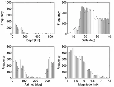
Table 2.1: Seismic data information used in this test Year Julian Day Origin Time Lat [deg] Lon [deg] Depth

[km] mb

(25)

To evaluate the reliability of the GUI being developed, tests for a set of Australian data were conducted. About 20 sets of three component seismic data for events recorded at stations SC02, SC04 and SC05 station from the SKIPPY experiment (1994) were employed. Information of this seismic data is shown in Table 2.1.

These three stations are selected because their geographical position is close to the Warramunga array, from which the seismic data of that have been analyzed by Gudmundsson et al. [1994] and Cheng [2000], thus our final result will be comparable with theirs.

For the calculation of the differential attenuation , the spectrum of the P

wave is estimated from the vertical component (Z) and the S waves spectra from the rotated components i.e. transverse (SH) and radial (SV) relative to the great circle between the source and receiver. Besides these waves, I also consider S waves spectra from a combined horizontal term

* SP

t

Δ

) (_SH2 _SV2

H = + .

The time window employed for the spectral estimation varies in length between 25s and 45s depending on the epicentral distance. Firstly P and S waves travel times are predicted by the ttimes software [Kennett and Engdahl, 1991] from which I compute

ak135 traveltimes [Kennett and Engdahl, 1995], then hand picking is used to obtain more accurate onsets. The spectral windows start at 1s before the P and 3s before the S

arrivals.

(26)

Figure 2.2

A snapshot of the Graph

ical User In

terface fo

r

S

to

P

dif

feren

tia

l attenua

tion estimatio

n measur

(27)

Figure 2.3

A snapshot of the Graph

ical User In

terface fo

r

P

to

P

and

S

to

S

diffe

ren

tial a

ttenu

(28)

As can be seen from equation (2.10) the differential attenuation between S and P

wave spectra can be obtained from the slope of the linear regression of the logarithm of the ratio of the amplitude spectra as a function of frequency. I use a frequency band of 0.10 to 1.0 Hz, and assume a weak dependence on frequency. In general the logarithmic spectral ratio is close to linear with frequency in this frequency band so that I can use a model in which attenuation is independent of frequency.

The penetration of the seismic ray path in depth increases as the epicentral distance increases. To see the behavior of average attenuation in the lithosphere, upper mantle and transition zone, examples of the estimation are shown at distances 12.4°, 19.9° and 26.1° in Figure 2.4(a), 2.4(b) and 2.4(c). Figure 2.4 (a) shows that at epicentral distance 12.4°, the frequency content of both P and S waves remain moderately high, suggesting that both seismic waves passed through low attenuation zone. Meanwhile, Figure 2.4 (b) shows a significant difference in the frequency content of P and S. The P waves remain moderately high frequency, but the S waves returned from the transition zone and below decay rapidly with increasing frequency. The features of frequency content of seismic waves in Figure 2.4 (c) are similar to that in Figure 2.4 (b).

* SP

t

Δ

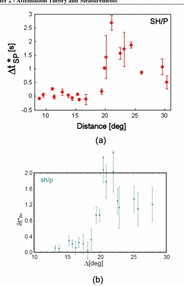
A compilation of the measurement for all data used in this test is illustrated in Figure 2.5 (a). The figures show that, the frequency decay rates of P and S wave varies with the epicentral distance. It can be seen that the consistently low value of the out to a distance of 18°, followed by a sudden increase of the between distances of 18° and 21° and gradual decrease beyond the distance of 21°. The features show a good agreement with the previous study of the measurement of Warramunga data conducted by Cheng [2000] (Figure 2.5 (b) and Gudmundsson et al.

[1994] (see Figure 3.9 (a)).

(29)

(30)

[image:30.595.105.513.192.650.2]

(31)

(c)

Figure 2.4:

Examples of seismic sig

nals reco

rded at the SC05

station with different ep

icentral d

is

tances an

d

the vertical, radial, transverse

and ho

rizon

tal wav

e spectra an

d the spectral ratio meas

uremen

[image:31.595.107.502.190.652.2]

(32)

[image:32.595.128.497.73.646.2]

Figure 2.5: (a)Plotofmeasurements of logarithmic slope of spectral ratio as a function

(33)

The GUI is also applied to seismic datasets which are recorded from the recent project (TASMAL project, 2004). I choose 4 high quality datasets recorded by TL01 station. TL01 station is situated near the Tasman Line which is the line of separation of old Precambrian rocks in the central-west Australia from younger rocks in eastern part.

Figure 2.6 (a) azimuth: 70.65º; epicentral distance: 20.27º

(34)

(c) azimuth: 293.53º; epicentral distance: 21.95º

(d) azimuth: 333.73º; epicentral distance: 19.13º

Figure 2.6: The S to P differential attenuation (∆t*SP) estimation for TL01 station, P

(35)

(See Chapter 3 for more detail). The seismic events are taken for different azimuths relative to the station location. Figure 2.6 shows the ∆t*SP estimation for TL01 station.

The results of these measurements suggests that there is a correlation between values of the ∆t*SPand lithological features. The ∆t*SP results from the east (Figure 2.6 (a) and

(b)) which are associated with young oceanic region, decay rapidly compare to paths from the west (Figure 2.6(c) and (d)) which are associated with the old cratonic region. All of these seismic paths are plotted in Figure 2.7.

Figure 2.7: Seismic paths from four events (red triangles) discussed in Figure 2.6 above

recorded at TL01 station (blue star) which is located around Tasman Line location (blue dotted line). The tectonic boundaries are illustrated in red lines. Note that the ∆t*SP paths

from the east are higher than those from the west.

(36)

used as a reference. The values of and estimated from each station is also shown in the Figure.

* PP

t

Δ *

SS

t

Δ

Note that SA04 station which is located to the west of the Tasman Line has lower and than SA05 which is located to the east. This suggests that seismic waves traveling to SA04 are less attenuated than those traveling to SA05.

* PP

t

Δ *

SS

t

Δ

Representations of the application of the Station Ratio Method for each station are shown in Figure 2.9 (a), (b), (c) and (d) below. The top panel shows seismic data in time domain for vertical, radial, transverse and horizontal components. The left-bottom panel shows close up of P waves, its spectra and the estimation. The P waves and spectra of reference are drawn in red and the estimated data are in blue. The background noise spectra are drawn in green. The right-bottom panel shows estimation along with the value of each differential attenuation measurement and error in the estimation.

* PP

t

Δ

* SS

t

Δ

Figure 2.8: Seismic event and seismic station locations and great circle between the

(37)

(a)

(b)

(38)

(c)

(d)

Figure 2.9: The P to P and S to S differential attenuation ( and ) estimation

for the seismic data from an event in Irian Jaya recorded by SA04, SA05, SA06, and SA08 stations. (a) Estimation of the and for SA04 relative to itself (reference) resulting and equal to 0, (b), (c) and (d) the estimation of SA05, SA06 and SA08 respectively.

* PP

t

Δ *

SS

t

Δ

* PP

t

Δ *

SS

t

Δ *

PP

t

Δ *

SS

t

(39)

Chapter 3

Australasian Setting and Previous Seismic

Studies of Australia

“Everyone is a product of their own experience. Hence geophysicists tend to favor geophysical methods and geologists tend to favor geological methods. It’s only natural” [Brown, 2005].

The Seismologists observe seismic signals which have traveled through the

earth. They analyze and manipulate this signal to understand geological features of the

earth. Since correlation between the signal and earth features is not perfectly straight

forward, a basic knowledge of geological features is needed to avoid misinterpretation.

In this Chapter, a broad outline of Australian geology and its tectonic setting is

described. Also, geological interpretations from previous seismic studies are presented.

This knowledge will be used as a platform for the interpretation of geological features

of Australian regions from the attenuation images produced in this research.

3.1 Australian Setting

3.1.1 The Australian Continent

Based on studies of rocks at the surface, in general, the structure of the

Australian continent is divided into three divisions which mark major stages in the

evolution of the crust: the Archaean (older than 2500 Ma), the Proterozoic (2500-550

Ma) and the Phanerozoic (younger than 550 Ma). The Major Archaean outcrop lies in

(40)

Chapter 3 - Australasian Setting and Previous Seismic Studies of Australia 31

the west and the Proterozoic rocks are found in the east of the continent (Figure 3.1).

The Australian Continent is characterized by several cratons: Pilbara Craton, Yilgarn

Craton, Gawler Craton, Curnamona Craton and Kimberley Craton. The Yilgarn Craton

is characterized by granite-greenstone belts bounded by major strike-slip faults and

shear zones, the south-western gneiss terranes and the gneissic Narryer terrane in the

northwestern part of the craton. Based on seismic reflection data over the eastern

Goldfields Province, it suggested that there is a three-layered crust [Drummond et al., 2000]. The uppermost layer is formed by greenstone belts in the central and eastern

parts of the section. The mid-crustal section (10-20km) consists of an east-dipping, west

vergent duplex system, whereas the lower crust is characterized by shallowly dipping

reflectors that are interpreted to represent ductile deformation [Drummond et al., 2000]. The seismic reflection data also shows that the crustal thickness of the Yilgarn and

[image:40.595.110.515.423.699.2]

Pilbara Cratons is between 30 and 35 km thick [Betts et al., 2002].

(41)

The Pilbara Craton is located to the north of the Yilgarn Craton comprises a

central granite-greenstone belt characterized by a outcrop pattern dominated by 50-100

km diameter domal granitoid complexes, separated by synformal greenstones belts

[Oliver & Cawood, 2001]. The Pilbara Craton consists of a series of early to

mid-Archaean to Paleoproterozoic strata of the Hamersley Basin [Hickman, 1983].

Between the Pilbara and Yilgarn Cratons there is the Carpicorn Orogen which is

characterized by regional metamorphism and plutonism with the main activity ending at

1840 Ma [Myers et al., 1996]. According to the teleseismic receiver functions study of Reading & Kennett [2003] with three-component temporary stations were deployed in a

line running southwards across Pilbara Craton, Capricorn and Yilgarn Craton, it is

suggested that the crust-mantle boundary under the Pilbara Craton is shallow, at 30 km,

with a sharp Moho and high-velocity crust beneath the exposed Pilbara

granite-greenstone terrane. The Yilgarn Craton which extends beneath the basins exposed on

the surface is deeper at 40 km. An anomalous region exists under the Southwest terrane

which shows a thick high-velocity gradient zone at the base of the crust and a Moho

dipping to the west. The character of the lateral heterogeneity in structure and its

correspondence with terrane boundaries suggest that accretionary processes are

significant in the evolution of the Yilgarn Craton.

In the south Australian region there is the Gawler Craton which is part of a

complex collage of Archean to Mesoproterozoic metasedimentary and metaigneous

terranes in southern Australia [Direen et al., 2005]. The core of the Gawler Craton is comprised of Archean gneissic complexes, whose protoliths may be as old as 2.98 Ga

[Dawson et al., 2002].

The evolution of Tasmania region began as long ago as 800-750 Ma [Turner et

al., 1998], with prolific granite on King Island and deposition of thich turbidite sediment in North West Tasmania. Western Tasmania was formed in the Middle to Late

Cambrian Tyennan Orogeny. The east of Tasmania contains no evidence of the

(42)

beneath Tasmania has been investigated using teleseismic tomography by Rawlinson et

al. [2006]. They used 6520 relative P wave arrival time residuals from 101 distant earthquake recorded by 72 seismic recorders. Their images show marked transition from

higher seismic speeds in the east to lower speeds in the west. Furthermore, the Tamar

Fracture System does not overlie the narrow transition from relatively fast to slow

speed. Farther in west region, an easterly deeping zone of relatively high velocity

material beneath Rocky Cape Group and Arthur Lineament may be related to remnant

subduction of oceanic lithosphere related with the mid-Cambrian Delamerian orogeny.

In the eastern part of Australian Continent, there are three major Orogens: the

Lachlan, New England, and Thompson Orogens. The Lachlan Orogen is a

turbidite-dominated orogen that forms the central part of the composite Palaeozoic Tasman

Orogen [Coney et al., 1990] along the eastern margin of Australia. Successive cratonisation from west to east included the Early Palaeozoic Delamerian Orogen

(550-470 Ma), the Middle Palaeozoic Lachlan Orogen (450-340 Ma) and the Late Palaeozoic

to Early Mesozoic New England Orogen (310–210 Ma), with their respective peak

deformations of Late Cambrian - Early Ordovician, Late Ordovician - Silurian and

Permian - Triassic age [Foster & Gray, 2000]. The Lachlan part is a Middle Palaeozoic

orogen with a 200 million years history that occupies ~50% of the present outcrop of

the Tasman Orogen [Gray & Foster, 2004]. The Lachlan and New England Orogens

belong to an orogenic system that extended approximately 20,000 km along the eastern

margin of Gondwana between the northern Andes and eastern Australia [Gray & Foster,

1998].

3.1.2 Surrounding Regions

In the surrounding regions of the Australian Continent there are several

geological and tectonic features such as the Tasman Sea, the Coral Sea, the New

(43)

East Indian Ridge, the West Australian Basin, the Lord Howe Rise, the Macquarie

Ridge, and the Indian-Antarctic Ridge (Figure 3.2).

The Tasman Sea is located to the east of the Australian Continent, it is an ocean

basin which is bounded by the Lord Howe Rise and New Zealand to the east and to the

south by major discordance that separates it from younger oceanic crust generated at the

South East Indian Ridge and the extinct Macquarie Spreading center. In the northern

part, it contains an elongated segment of continental crust, the Dampier Ridge which is

separated from the Lord Howe Rise by two small basins: the Lord Howe and the

Middleton basins. Based on tectonic lineaments visible in the gravity grid and

interpreted as strike-slip faults, by magnetic anomaly, bathymetry, and seismic data,

Gaina et al. [1998] identified 13 tectonic units. These 13 tectonic blocks and the Australian continent gradually separated due to either extensional or strike-slip

movements, generating the Tasman Sea, the Lord Howe and the Middleton basins, and

several failed rifts. The opening of the northern Tasman Sea is pretty well explained by

the gradual stepwise separation of four Dampier Ridge tectonic fragments plus the

Chesterfield Plateau and Australia in the frame work of a northward propagating rift.

Another major oceanic basin which borders the Australian margin to the east is

the Coral Sea. The Coral Sea Basin is located northeast of Australia and is rimmed by

several submarine plateaus such as the Queensland Plateau to the southwest, to the

northwest by the Eastern Plateau, the Papuan Plateau to the North, the Louisiade Plateau

to the northeast, and the Mellish Rise to the southeast. The Coral Sea basin is formed by

Early Eocene oceanic crust [Gaina et al., 1999].

According to magnetic anomaly interpretation and fracture zone data revealed

from satellite-derived gravity anomalies, Gaina et al. [1999] derived finite rotations for the Coral Sea opening. These rotations are combined with the previous work of Gaina

(44)

Plate, Lousiade Plateau and several small plateaus attached to the northern Lord Howe

Rise.

Figure 3.2: Geographic and Tectonic features in the surrounding regions of the Australian Continent [digital data courtesy of NOAA].

To the south of the Australian Continent, there is the Australian Antarctic

Discordance which is a zone of subdued ridge morphology and a series of north-south

trending fracture zones [Weissel & Hayes, 1974]. The Australian Antarctic Discordance

is the deepest portion of the mid-ocean ridge system over a 600km long segment of the

South East Indian Ridge. It is anomalous in terms of bathymetry and is characterized by

unusual sea-floor morphology, isotope geochemistry, petrology, and seismic structure

[Gurnis and Müller, 2003]. The Australian Antarctic Discordance has been associated

with the location of former Mesozoic position of long-lived seduction on the Pacific

margin of Australia. Seismic tomographic images suggest that beneath this former

(45)

mantle and a high velocity anomaly within the transition zone, as originally predicted

by dynamic models [Gurnis and Müller, 2003].

To the west of Australia, there is the West Australian Basin. This basin is the

oldest sea floor formed during the Jurassic (155 Ma). Based on surface wave study of

Fishwick [2005], beneath the old West Australian Basin, fast shear velocity

perturbations are determined.

To the north west of the continent, complex subduction zones exist between

Australian and Eurasian plates. Tomographic images of Widiyantoro [1997] reveal the

slab in the upper mantle resembles the present day Java trench, Timor trough, the

curved Banda arc, and the Molucca Collision Zone. This study also indicated the

presence of fast P wave speed beneath northern Australia.

3.2 Previous Seismic Tomography and Seismic Attenuation

Studies of Australia

Studies on seismic tomography of the Australasian region have exploited the

data availability from deployments of broadband instruments. In the SKIPPY

experiment from 1993 to 1996 [van der Hilst et al., 1994], recorders were deployed across the whole continent at approximately 400 km spacing. Subsequently in 1997 and

1998 a denser array of broadband instrument (KIMBA) were deployed in northwestern

Australia. In 1999 additional recorders were installed in southeastern Australia

(QUOLL). In 2000-2001, Western Australia was revisited with a broadly spread array

to supplement the SKIPPY stations which had had technical problems. In less than a

decade there has been a very thorough coverage of the Australian continent with

broadband seismic stations. The high quality seismic data availability at a suitable

distance from events in surrounding region with a dense stations spacing is ideal to

(46)

3.2.1 Tomography Studies of Australia

Tomography studies of Australia have been conducted by using many types of

seismic waves: surface waves, body waves, Lg coda, etc. Studies on surface wave tomography have been initiated by Zielhuis and van der Hilst [1996] by analyzing

Rayleigh wave data from the stations in eastern Australia deployed in the SKIPPY

experiment. Their model suggests the presence of a major contrast in the shear

wavespeed in the mantle component of the lithosphere between central Australia and

eastern Australia. The model revealed the presence of lowered shear wavespeeds

beneath the east coast of Australia at depths around 140km which has a strong

correlation with Neogene volcanism.

The Australian surface wave tomographic models have been improved as more

data have been incorporated by van der Hilst et al. [1998] and Simons et al. [1999]. The shear wavespeed distribution for SV waves at 140, 200 and 300km depths derived from this inversion are presented in Figure 3.3 below.

Shear wave velocity contrasts between eastern Australia and central Australia

(between 140ºE and 145ºE) is clearly pronounced at 140 and 200 depths and may be

associated with the controversial Tasman line. The zones beneath the exposed

Precambrian rocks in the west and central Australia are associated with high seismic

wavespeeds. The Precambrian regions show the presence of significant internal

structure with an indication of the separation of the major cratonic blocks, especially at

shallower depths. The high seismic wavespeed anomaly at 300 km depth is concentrated

in the central Australia. The seismic speed perturbation at this depth is less than the

shallower structure, this anomaly could be associated with real geologic features in the

upper mantle or might be correlated with the sampling pattern of lateral resolution.

Tomographic models from surface wave tomography was then improved by

Yoshizawa and Kennett [2004] by using more seismic data and introducing a

(47)

(48)

Figure 3.4: Shear wave speed model in the upper mantle. Reference velocities are 4.41 km/s at 100 km, 4.43 km/s at 150 km, 4.51 km/s at 200 km, 4.61 km/s at 250 km, 4.70 km/s at 300 km, and 4.75 km/s at 350 km [Yoshizawa and Kennett, 2004].

In general, the major features of Yoshizawa and Kennett’s tomographic models

are quite similar to those of the corresponding maps of van der Hilst et al. [1998]. Down to 200 km depth the cratonic slab in central and western Australia is characterize

by high shear velocity and the oceanic crust in eastern seaboard is characterized by low

(49)

The availability of three-component seismic data allows the exploitation of

polarization anisotropy beneath the Australian Continent. Debayle & Kennett [2003]

presented radial anisotropy in term of the ratio between tangential (SH) waves velocity and radial (SV) velocity. Their result is presented in Figure 3.5. As can be seen from the figure, at slice 125km depth, in the continental region of Australia and in the subduction

zones in the north, the value of the anisotropy is higher than 1 which is illustrated by

green color scheme. In such regions the polarization anisotropy is such that SH is faster than SV. The vertical cross section of the anisotropy at -25ºS suggests that at central and eastern Australia SH is faster than SV down to 200-250km. The area where SH is faster than SV is the eastern region may be associated with the part where horizontal flow dominates in the upper mantle.

(50)

The recent work on surface wave tomography has been conducted by Fishwick

[2005] as more data from all Australian National University temporary deployments and

additional data from permanent stations and temporary deployment in New Zealand are

incorporated.

Figure 3.6: Correlations between age and shear wave speeds anomaly in Australasian [Fishwick, 2005].

Figure 3.6 above shows the shallowest layer of the tomographic model in a slice

at 75km depth. The model suggests correlations between shear wavespeeds and

geological structures in the oceans surrounding Australia. Evidence from the depth of

the sea floor and the reduced heat flow away from mid-oceanic ridges suggests that the

oceanic lithosphere cools with increasing age. The image suggests that shear

wavespeeds increased with increasing age. Beneath the old West Australian Basin (A),

fast shear velocity perturbations are observed, and beneath the young Southeast Indian,

and Indian-Antarctic ridge system (B) much lower wavespeeds are imaged. To the east

of Australia, the fastest wavespeeds are observed beneath the Tasman and Coral Sea and

(51)

Figure 3.7: Correlations between Tasman Line concept and surface wave tomography at 150km depth [Fishwick, 2005].

The shear wavespeed slice at 150km depth derived from surface wave

tomography is presented in Figure 3.7 along with locations of proposed Tasman Lines.

At this depth the transition from slower to faster velocities is not a simple linear feature

and appear to be a somewhat complex boundary between 138ºE and 143ºE [Fishwick,

2005].

The seismic structure beneath the Australasian regions also has been analyzed

using seismic traveltimes tomography. Gorbatov and Kennett [2001] presented

compressional (P) and shear (S) waves models derived from a data set contains 544690

P-wave and 393866 S-wave ray paths. All arrival times were selected from the catalog which have source or receiver located within the zone of study (95ºE to 190ºE; 50ºS to

10ºN). Since calculations of 3D ray paths for a large amount of data are very time

consuming they combined the information from event clusters in a 2º x 2º x 50 km

volume and station clusters in a 2º x 2º region into a single summary ray path for the

(52)

Figure 3.8: P (left) and S (right) wave tomographic models derived from traveltimes tomography at 70-110km, 160-210km and 270-340km depth. The colorbar is presented in percent relative to ak135 model [Gorbatov and Kennett, 2001]

The residual time assigned to the summary ray was the median of all the

relevant data selected for summary ray path. Each summary ray was composed of at

least three individual rays. The resulting data set contains 544690 P-wave and 393866

S-wave ray paths. The region of interest was parameterized by irregular cells from 0.5ºx0.5º to 1ºx1º and 19 layers down to the depth of 1600 km. The whole Earth mantle

Seismic body wave attenuation tomography beneath the Australasian region