Structuring Statistical Tests for Validating Encryption: An Array-based Approach

Theses Thesis/Dissertation Collections

5-2016

Structuring Statistical Tests for Validating

Encryption: An Array-based Approach

[email protected]

Follow this and additional works at:http://scholarworks.rit.edu/theses

This Thesis is brought to you for free and open access by the Thesis/Dissertation Collections at RIT Scholar Works. It has been accepted for inclusion in Theses by an authorized administrator of RIT Scholar Works. For more information, please [email protected].

Recommended Citation

MASTER’S THESIS

Structuring Statistical Tests for Validating Encryption:

An Array-based Approach

Author:

Kevin Hoyt Dr. Peter Bajorski Advisor:

A 3 credit thesis submitted in partial fulfillment of the requirements for the degree of Master of Science in Applied Statistics

In the

John D. Hromi Center for Quality and Applied Statistics The Kate Gleason College of Engineering

Committee Approval

The undersigned have examined the thesis titled “Structuring Statistical Tests for

Validating Encryption: An Array-based Approach” by Kevin Hoyt, a candidate for the degree of

Master of Science in Applied Statistics, and hereby approve that it is worthy of acceptance:

Dr. Peter Bajorski Date

Thesis Advisor

Dr. Alan Kaminsky Date

Committee Member

Dr. Marcin Lukowiak Date

Declaration of Authorship

I, Kevin Hoyt, declare that this thesis titled “Structuring Statistical Tests for Validating

Encryption: An Array-based Approach” and the work presented in it are my own. I confirm that:

v This work was done wholly while in candidature for research at the Rochester Institute of

Technology.

v Where any part of this thesis has previously been submitted for a degree or any other

qualification at this university or any other institution, this has been clearly stated.

v Where I have consulted published work of others, this has been clearly stated.

v Where I have quoted the work of others, the source is always provided and with the

exception of such quotations, this thesis is entirely my own work.

v I have acknowledged all main sources of help.

v Where the thesis is based on work done by myself jointly with others, I have made clear

exactly what was done by others and what I have contributed myself.

“Knowing how to think empowers you far beyond those who know only what to think.”

ROCHESTER INSTITUTE OF TECHNOLOGY

Abstract

The Kate Gleason College of Engineering Master of Science

Structuring Statistical Tests for Validating Encryption:

An Array-based Approach

by Kevin Hoyt

The technological advancements made in recent years regarding the transfer of personal

data have brought along an imperative need for increased security and encryption capabilities.

Information sent across these electronic platforms is most often intended to be delivered to and

received by specific individuals. However, the notion that these selected individuals are the only

people that are able to come into contact with the information is flawed. A more realistic

assumption, and the assumption that is currently demonstrated, is that the information sent can

and will be intercepted. This means that successful encryption of the data is an invaluable part of

the transfer process. For this reason, the study of encryption and the validation of cryptographic

functions are topics that computer scientists continually work to improve. Current practice for

determining the success of cryptographic functions tends to consist of various statistical tests

conducted on random outputs from the algorithm. In this thesis, we propose an array-based

structure to validate not only the output from an cryptographic function, but the cryptographic

function itself. In using an array-based structure such as this, we do not limit ourselves to only

detecting output that suggests a failure for the encryption function. With this structure we allow

Acknowledgements

I would like to thank my advisor Dr. Peter Bajorski for the opportunity to collaborate

with him on this project and for his endless support and assistance throughout the entire process.

I truly am grateful for his contribution of knowledge and his commitment to me as I continually

gained more and more understanding. I am also appreciative of his kindness and patience with

me as I was able to juggle this project alongside others in my life. He truly is a great person and I

cannot thank him enough.

I would also wish to thank Dr. Alan Kaminsky for the opportunity to assist in working on

the Harris project along with all of those that worked on the project as well. That project helped

to direct me to this research and all research that has been conducted alongside it. I would also

like to thank him for the acceptance of being on my thesis committee and his previous work in

the field, which I was able to study more in depth.

I would also like to thank the John D. Hromi Center for Quality and Applied Statistics for

accepting me as a student in the master’s program and for the John D. & Rachel E. Hromi

Endowed Scholarship as well as the opportunity to work as a teaching assistant while attending.

Also, I wish to thank all faculty and staff in the department that assisted me or taught me during

my time there.

Finally, I would like give my deepest thanks and love to my wife for putting up with me

and my crazy idea of going back to school full-time while she supported us. She has been

understanding and supportive throughout these past few years. She is an amazing wife and I

List of Figures

Figure 1: Basic overview of encryption  ...  3  

Figure 2: Kaminsky's block cipher coincidence test [1]  ...  9  

Figure 3: Example of Kaminsky's Coincidence Test H1 distribution  ...  11  

Figure 4: Power of coincidence test with varying n-values  ...  13  

Figure 5: Array-based testing structure  ...  15  

Figure 6: Probability mass function for binomial distribution  ...  18  

Figure 7: Compressed array-based testing structure  ...  21  

Figure 8: Power of tests applied to Model 1  ...  23  

Figure 9: Power of tests applied to Model 2  ...  24  

Figure 10: Power of tests applied to Model 3  ...  25  

Figure 11: Precision for proportion = 0.5  ...  27  

Figure 12: Comparison of analytical and simulation results for Model 1, 64-bits  ...  28  

Figure 13: Test 3 Simulation errors and analytical results for Model 1  ...  29  

Figure 14: Comparison of analytical and simulated results for Model 2, 64-bits  ...  30  

Figure 15: Comparison of analytical and simulated results for Model 3, 64-bits  ...  30  

Figure 16: Test 3 simulation errors and analytical results for Model 2  ...  31  

Figure 17: Test 3 simulation errors and analytical results for Model 3  ...  31  

Figure 18: Exact binomial power calculations, Option 1  ...  34  

Figure 19: Exact binomial power calculations, Option 2  ...  35  

Figure 20: Exact binomial power calculations, Test 3, option 1  ...  38  

List of Tables

Table of Contents

Committee Approval  ...  i  

Declaration of Authorship  ...  ii  

Abstract  ...  iv  

Acknowledgements  ...  v  

List of Figures  ...  vi  

List of Tables  ...  vii  

Table of Contents  ...  viii  

1. Overview and Organization  ...  1  

1.1 Overview of the Project  ...  1  

1.2 Thesis Organization  ...  2  

2. Encryption Overview  ...  3  

3. Outline of Statistical Errors and Power of the Tests  ...  6  

4. Analytical Power of Kaminsky’s Coincidence Test  ...  8  

5. Array-based Testing Structure  ...  14  

6. Binomial Test and Error Correction  ...  17  

7. Application of Array-based Binomial Tests  ...  21  

8. Simulated Results for Array-based Tests  ...  27  

9. Investigations of Discreteness and Bit-length for Binomial Testing  ...  33  

10. Conclusion and Future Work  ...  40  

Bibliography  ...  42  

1. Overview and Organization

1.1 Overview of the Project

This project began as an investigation of statistical testing for encryption in the field of

computer science. To gain necessary insight on the overall process of encryption, research was

conducted to become better familiarized with the basic encryption process. However, micro-level

research regarding the development and implementation of cryptographic functions and

algorithms was left to those in computer science. Of such research was Dr. Alan Kaminsky’s

recent contribution to the field of computer science with the development of the Coincidence

Test, a Bayesian application of statistical randomness testing for block ciphers and message

authentication codes (MACs) [1]. To better understand the process, his test was dissected at the

statistical level to determine how the errors within the test behaved and how they could be

controlled, if at all possible. The results of the initial investigation led to the analysis of the

power of the Coincidence Test, which is a metric that could then be compared to other tests.

It was then decided that the development of an alternate testing scheme may assist in

controlling errors, while also detecting components of the cryptographic functions that contribute

to failures in the test. This testing scheme, which we title “array-based”, was established on a

factorial design structure, which is the foundation for the theory of experimental design. To

investigate the structure, a binomial distribution was used, where the proportion of “1”s within a

sequence of “0”s and “1”s as obtained from an encryption method was hypothesized and tested.

This allowed to further investigate the nature of the test as it related to the array-based scheme,

Further examination was then necessary, specifically regarding the binomial test, due to the

discreteness of the data in the simulations as they compared to the normal-approximation to the

binomial distribution for the analytical results. Finally, since the simulations best represent the

output from an actual encryption process, it was then necessary to further delve into the

simulations and the errors derived from the test.

1.2 Thesis Organization

In Chapter 2, we introduce the basic research conducted to better understand the process

of encryption. Chapter 3 focuses on different types of statistical errors regarding hypothesis

testing. We also introduce the connection between statistical errors the power of the tests

conducted. Chapter 4 first describes Dr. Alan Kaminsky’s Coincidence Test and then

demonstrates the underlying distribution of the test and the power of the test under various

scenarios. In Chapter 5 we introduce our array-based testing scheme and the multiple tests that

can be arranged from such a structure. Chapter 6 first briefly explains the binomial test and then

follows with describing the necessary error adjustments needed for multiple testing. Chapter 7

describes the three basic models that are available to test using the array-based testing structure.

It then demonstrates the application of the Normal-approximation to the binomial distribution to

obtain analytical results for the power of the tests used for the three models. In Chapter 8 we

demonstrate the simulated results from the three models and make comparisons to the analytical

results. Chapter 9 describes the discreteness dilemma that is apparent in the simulations, and the

treatment of the errors in such cases. Finally, Chapter 10 concludes the paper by describing

2. Encryption Overview

The application of cryptography, or at least its relationship to the science of encryption, is

not new [2]. For centuries, the transfer of surreptitious information has been critical to the

success of empires and businesses throughout the world. From ancient communications

regarding military warfare processes to today’s current need for online security, cryptography

has played a major role in allowing crucial information to be passed from sender to recipient

without much fear of extraction from those able to intercept it. Recently, with growth in the field

of computer science, success of encryption has become increasingly desirable as much

communication regarding the personal and financial information of individuals continues to shift

toward a wireless realm. Along with this ever evolving need for superior encryption techniques

comes also a demand for methods of testing the success or validity of the encryption process. It

is often the case that computer scientists gauge the success of an encryption technique with the

output that comes from the encryption system.

The general idea of encryption is fairly basic, though the underlying processes and

techniques used by those in the computer science field are advanced and are beyond the scope of

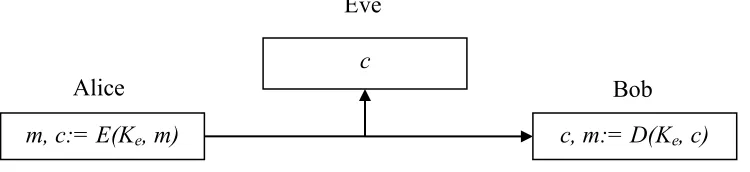
this paper. In short, the idea is often explained using an example with arbitrary participants Alice

(the sender), Bob (the recipient), and Eve (the interceptor) of a particular message [2].

Figure 1: Basic overview of encryption

c

m, c:= E(Ke, m) c, m:= D(Ke, c)

Alice

Eve

Here we can see that Alice has a message m, also known as the plaintext, which she

would like to send to Bob. The drawback is that Eve may be receiving the message as well. In

order to protect from the possibility of Eve obtaining the message directly, an assumption is

made that Eve, as well as Bob, will be receiving anything that is sent on the channel. Alice can

then create a ciphertext c from an encryption function E(Ke, m) by using a key Ke that is only

shared with Bob. This ciphertext is then sent along the channel, where it is assumed that both

Bob and Eve receive it. Since Bob has Ke, and Eve does not, Eve has no means of revealing the

plaintext message, she can only view the ciphertext created by Alice’s and her encryption

function. However, Bob can use a decryption function D(Ke, c) to decrypt the ciphertext and

obtain the plaintext m. In the field of computer science, encryption is considered successful in

the event that Bob can determine a plaintext sent from Alice while Eve cannot.

This focus contributes to many of the advancements within the field. Though it would be

really simple if we could assume that an individual or more realistically, a machine, intercepting

a ciphertext could not determine the plaintext without the given key, this is not nearly the case.

Cryptographic functions that use weak keys or struggle encrypting specific key and plaintext

combinations are susceptible to attacks from interceptors, which can detect patterns in the

ciphertexts to establish the plaintexts without the key. In computer science, encryption

algorithms create ciphertext strings consisting of binary sequences of specific bit lengths.

Theoretically, in order to be successful, these ciphertexts would then appear to be strings of

completely random binary bits. That is, the binary sequences would not have detectable patterns

that the interceptors would be able to use to decrypt the messages. The behavior of the bits

within the ciphertexts created is something that computer scientists investigate in the quest for

by the algorithms and these samples are then used to determine the validity of the encryption

techniques in their regard to this success. These sample-based tests are worthy of determining the

randomness of the outputs, however there lies an issue with the effectiveness of the

cryptographic function, and more importantly the performance of the function with specific keys

and/ or plaintext. There are possibilities for outputs to appear random, when in fact they are

developed from the combination of random plaintexts and weak keys. An operational way to

determine the ineffectiveness of the cryptographic function with particular keys and/or plaintext

encrypted within the algorithm is to create an array-based test, to focus on the combinations of

plaintexts and keys, and thus the overall success of the cryptographic function. To note, for the

remainder of this paper, the use of “validation of encryption” or “encryption algorithm” is done

regarding the validation of the specific cryptographic function that would be the receiving the

3. Outline of Statistical Errors and Power of the Tests

Statistical hypothesis testing can be applied to the testing of the success of the encryption

algorithms. This can be done by using a variety of tests from different origins, each with

different detection capabilities. Traditionally, frequentist testing has assumed fixed parameters

to see if the data provided fit the parameters. More recently, Bayesian testing has assumed fixed

data to see if the parameters are reasonable for that data. Both forms of testing are valid,

however, with any statistical testing, it is important to know that there are also possibilities for

errors within the tests, and that these errors contribute differently within the testing scheme.

Hypothesis testing consists of either providing statistical evidence for the rejection of a

null hypothesis H0, in favor of an alternative hypothesis HA, or not providing statistical evidence,

and therefore not rejecting H0. Though the statistical evidence will vary by the test, the way in

which errors can be committed for the testing does not vary. For each of these errors it is also

important to know that when we use a test, the reality is that either H0 is or is not in fact true.

• Type I Error 𝛼 : The probability of rejecting H0, in the event that H0 is actually true.

• Type II Error 𝛽 : The probability of not rejecting H0, in the event that H0 is actually

false.

Both of these errors have different levels of importance based on the test conducted and

the relevant hypotheses. These levels of importance are taken into consideration when deciding

when conducting a test, but inference is hindered when acceptable error rates are not taken into

careful consideration.

Lastly, when considering our tests, we are interested in knowing their power.

• Power of the test 1−𝛽 : The probability of rejecting H0, in the event that H0 is actually

false.

This is especially important in comparing different tests to each other for their detection

capabilities. That is, if a null hypothesis is indeed false, we would like for our test to able to

detect it and provide evidence so that we can correctly reject it. For this reason, the power of the

4. Analytical Power of Kaminsky’s Coincidence Test

Many frequentist-based statistical test suites exist within the field of computer science to

evaluate randomness of encryption mapping. The statistical test suite provided by the National

Institute of Standards and Technology (NIST) is one such suite comprised of 15 individual

statistical tests for randomness of outputs of the encryption algorithm when used as

pseudo-random number generators (PRNGs) [3]. These NIST tests make pseudo-randomness assessments on

entire strings of bits or blocks of the strings, depending on the particular test used. In general,

this package of tests is considered the basis for statistical randomness testing for computer

science, though performance of NIST is not considered robust in cases where block ciphers or

message authentication codes (MACs) are used [1]. Progress was made in regard to this issue by

Alan Kaminsky in 2013, with the development of the Coincidence Test, which implements

Bayesian statistical techniques specifically for block ciphers and MACs [1].

The Coincidence Test, as described and defined by Kaminsky, assesses the randomness

of the mapping of a (plaintext, key) to ciphertext for block ciphers. To complete this task, the test

utilizes a comparison of groups of output bits G, where g = |G| is the total number of bits in the

group, from an output value for a block cipher V with a ciphertext output C created by the

encryption of a plaintext P with key K. Coincidences occur in cases where the corresponding

group of output bits selected G, match for both V and C. The test completes n Bernoulli trials

with a single randomly chosen P along with n different randomly selected K values and

determines the frequency of coincidences k that occur. If the aforementioned mapping is indeed

random, the probability of the occurrence of a coincidence for a Bernoulli trial is p = 2- g_{. The}

• H1: a model with the probability of success equal to p = 2- g, and

• H2: a model with a probability of success other than p = 2- g.

The following figure taken from Kaminsky’s paper illustrates the idea of a coincidence as

previously defined.

Figure 2: Kaminsky's block cipher coincidence test [1]

The criteria for choosing the binomial model as previously mentioned comes from the

utilization of the posterior odds ratio, Bayes factors and prior odds ratios adapted from a ratio of

the respective applications of Bayes theorem:

𝑝𝑟 𝐻 𝐷 =  𝑝𝑟 𝐷 𝐻 ∙𝑝𝑟(𝐻)

𝑝𝑟(𝐷)

𝑝𝑟(𝐻!|𝐷)

𝑝𝑟(𝐻!|𝐷)=

𝑝𝑟(𝐷|𝐻!)

𝑝𝑟(𝐷|𝐻!)∙

𝑝𝑟(𝐻!)

𝑝𝑟(𝐻!)

Since H1 is a model with the probability of success of each Bernoulli trial equal to p, we have a

binomial distribution for H1 where

𝑝𝑟 𝐷 𝐻_! = !! !!!!! !𝑝

!_(1−𝑝)!!! _{, [1].}

Also, since H2 is a model with the probability of success of each Bernoulli trial equal to

something other than p, this probability is denoted as θ. Thus,

𝑝𝑟 𝐷 𝐻_! = !! !!!!!!𝜃

!_(1−𝜃)!!!_𝑑𝜃

!

! =

!

!!! , [1].

It then follows that the Bayes factor is

!"(!|!!) !"(!|!!)=

!!

!!!!!!𝑝!(1−𝑝)!!!∙(𝑛+1)  , [1]

and in the effort to save computational resources, the log is then taken to be

𝑙𝑜𝑔!"(!|!!)

!"(!|!!)=𝑙𝑜𝑔Γ 𝑛+1 −𝑙𝑜𝑔Γ 𝑘+1 −𝑙𝑜𝑔Γ 𝑛−𝑘+1 +𝑘𝑙𝑜𝑔𝑝+ 𝑛−𝑘 log 1−𝑝 +

with application of the gamma function substitution for the factorial. This is then, as described

by Kaminsky, equal to the log posterior odds ratio when multiple runs of the test are completed,

with an assumption that pr(H1) = pr(H2).

Finally, the log posterior odds ratio is then the sum of all log Bayes factors and the data is

said to support H1 when the sum of the log Bayes factors is greater than 0, and H2 otherwise.

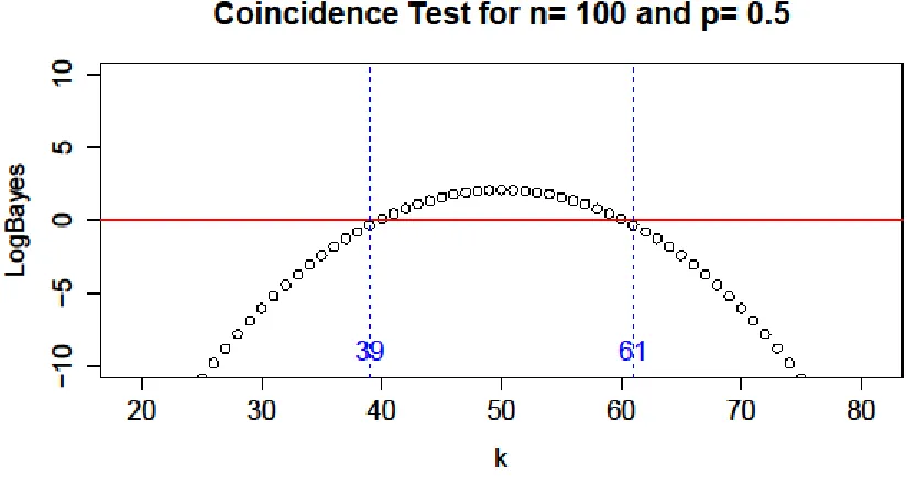
To demonstrate this, the possible log Bayes factors as a function of k are exhibited in

figure 3. In this example, we can see that when the test completes n = 100 independent Bernouilli

trials, and the underlying probability p = 0.5, the data supports H1 when 40≤𝑘≤60. However,

when 𝑘 <40  𝑜𝑟  𝑘>60, H1 is rejected and the data is said to support H2.

Figure 3: Example of Kaminsky's Coincidence Test H1 distribution

This simple example is meant only to show the basic principles of the coincidence test.

same manner with this test. As we can see in the figure, if H1 were in fact true, and 𝑘<40  𝑜𝑟  𝑘 >

60, then we would commit an error. In a traditional sense, we would set the value for 𝛼, which

would then provide critical values for k (something that will be demonstrated later). This is not to

say that by utilizing the log Bayes factors, control is entirely lost. On the contrary, by assuming a

cutoff value of 0, there is governance in the considerations for model selection, and thus the

errors committed by the test, but in a slightly different way. In fact, for the example shown in

figure 3, the calculation of the type I error is 𝛼=0.0352002.

As with any underlying discrete distribution, the true acceptable type I errors will be

dependent on integer-based critical values. Thus varying values of n within the test will lead to

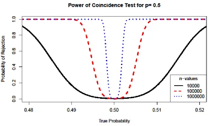
differing 𝛼 values. To demonstrate this, figure 4 compares the power of the coincidence test at

varying values, 𝑛=10!_,10!  _{𝑎𝑛𝑑  10}!_{. What is clear from the plot is that as n increases, the test is}

better able to detect slight differences from the assumed probability of H1, though careful

5. Array-based Testing Structure

As previously discussed, a randomness principle exists in the fact that evidence of

randomness in the outputs is not necessarily proof that there exists randomness of the

cryptographic function. There lies an essential issue with tests such as those within the NIST

suite for this reason. These tests are susceptible to the randomness principle since they can be

used as ways to identify randomness in sequences of the outputs, however understanding the

randomness capabilities of the cryptographic function is not even a possibility. The testing of

randomness from the outputs is an inefficient way to conduct these tests because these tests will

make conclusions that either randomness exists, or non-randomness exists. In an event that the

test shows that randomness exists, we are still hindered by the randomness principle, and we

really still know nothing about the cryptographic function that was used to produce the output.

On the other hand, if the test shows that there is non-randomness lurking in the output, we then

know that there is insufficiency in the cryptographic function, but the likeliness of

non-randomness occurring for a random combination of plaintext and key is extremely low, so we do

not really learn anything about the underlying issues. To combat this and attempt to focus on the

randomness of the cryptographic function, we introduce an arrangement for testing non-random

combinations of plaintexts and keys in the form of an array.

A common practice in experimental design is to test all combinations of factors within a

process to determine the factor levels that produce the most desired results. In doing so,

discoveries can be made in regards to the most optimal levels for each individual factor that may

controlled manner. Though the analysis is technically different, this same procedure can be used

for testing randomness in cryptographic functions.

Figure 5: Array-based testing structure

By investigating the ciphertexts produced by non-random combinations of plaintexts and

keys, we can determine if the cryptographic function struggles with particular keys, or if certain

plaintexts are difficult for a number of keys to properly encrypt. In this way we do not only have

an outcome from the test of random or non-random, but we will be able to determine specific

keys or plaintexts that are leading to the failure of randomness within the algorithm if that is the

The structure for such testing is what we refer to as array-based, since the outputs created

from the encryption function by each combination of plaintext and key are stored dimensionally

as an extension of the cell that contains the plaintext/ key combination. Here we can see in figure

5, that for our testing, the array is three-dimensional, with definitions of plaintext m, key k, and

bit n.

Many of the statistical tests that are currently used in practice can then be applied to this

structure. Tests can then be performed on any meaningful combination of the bits produced. For

example, using the test of our choice we can assess the randomness of the string consisting of all

𝑛𝑘𝑚 bits that were produced, investigate the randomness of the bits created 𝑘𝑛 for only one

particular plaintext, or look at other combinations as they are deemed necessary. In this way we

control the testing, which gives us more opportunity to detect faulty contributors to the

6. Binomial Test and Error Correction

One simple, yet very important test that should be applied to our aforementioned

array-based structure is the exact binomial test. The exact binomial test, is a frequentist-based exact

hypothesis test used to determine if a random variable X follows the binomial distribution where

the probability mass function is shown to be:

𝑃 𝑋=𝜔 = _𝜔𝑛 𝑝𝜔 _1−𝑝 !!𝜔  

We see that the distribution, which is modeling the number of successes 𝜔, in a sequence

of trials, is parameterized by the number of independent Bernoulli trials n, and the probability in

which a success occurs for each trial p. For our application we can define X to be the total

number of “1”s that occur in a sequence of n bits. If the probability of each “1” occurring is p,

then it is expected that np “1”s would occur in the string of bits tested. However, since natural

variation from the mean exists by chance, we understand that although a random variable

following the binomial distribution may have the highest probability at np successes, the random

variable can take on values that differ from this mean. For an example, in figure 6 we can see

that a random variable following the binomial distribution with n = 100 and p = 0.5 shows the

probability is highest for 𝜔=50. However, the probability that 𝜔=49 or 𝜔= 51 differs only

slightly. This means that in regards to hypothesis testing, we need to carefully determine critical

to assign a level of confidence that the random variable in question does indeed follow the

binomial distribution.

Figure 6: Probability mass function for binomial distribution

For any individual hypothesis test, we have a null hypothesis that is or is not true. In the

event that the null hypothesis is true we set the significance level 𝛼, which is an acceptable

probability for wrongfully rejecting the null hypothesis, or committing a type I error, based on

the test that is used. When set fairly low, the probability of not rejecting a true null hypothesis,

or not committing a type I error, is then 1−𝛼. We would like to have the probability of not

committing a type I error as close to 1 as possible, however when we conduct a series of t

𝑃 𝑛𝑜𝑡  𝑐𝑜𝑚𝑚𝑖𝑡𝑡𝑖𝑛𝑔  𝑎  𝑡𝑦𝑝𝑒  𝐼  𝑒𝑟𝑟𝑜𝑟 = 1−𝛼 =(1−𝛼)! !

!!!

With that,

lim_!→!(1−𝛼)! _{=0, 𝑓𝑜𝑟  0<𝛼<1,}

which is a major concern.

To correct this issue, we assume that each individual test conducted is independent and

we use the Sidak correction for multiple comparisons. Under this assumption we can determine

individual test significance levels 𝛼! to be a function of the overall family significance level 𝛼!

and the number of tests to be conducted t:

𝛼_! =1− 1−𝛼_! !!

Then when a series of t tests are conducted, we have overall significance for the series of tests if

any individual test is significant at the 𝛼! level.

For our situation and its relation to the binomial test, we assume that within the binary

sequences of ciphertext created by the encryption function, the proportion of “1”s in each

individual sequence should be p0. In other words, our hypotheses are:

𝐻!:𝐹𝑜𝑟  𝑒𝑎𝑐ℎ  𝑏𝑖𝑛𝑎𝑟𝑦  𝑠𝑒𝑞𝑢𝑒𝑛𝑐𝑒  𝑜𝑓  𝑐𝑖𝑝ℎ𝑒𝑟𝑡𝑒𝑥𝑡,𝑝=𝑝!

To test these hypotheses, we can begin by selecting an acceptable overall error-rate 𝛼!,

which we can use to make a determination for 𝛼! by incorporating Sidak corrections. Also, since

𝐻_! specifically suggests that 𝑝≠𝑝_!, we have a two-tailed test, which means that:

𝛼!

2=!!!!!! ! !

! .

Since we assume that X follows a binomial distribution, the cumulative distribution is

𝐶𝐷𝐹=𝑃 𝑋≤𝑎 = ! _𝜔𝑛 𝑝! _1−𝑝 !!!

!!! ,

where n is the total number of bits in the sequence, 𝜔 is the number of “1”s, and p is the

probability of success p0. Also, a is the value that X, the random variable can take on, such that

the probability is the sum of a discrete cases. Then we can obtain the critical values for each

individual test using the CDF and 𝛼!. Again, if any individual test fails at that level, then we can

7. Application of Array

-

b

ased Binomial Tests

To demonstrate the importance of the array-based testing structure, we introduce three

models for non-randomness in the encryption function as applied to the binomial test.

• Model 1: 𝑝≠ 𝑝! for all kmn bits within the testing structure

• Model 2: 𝑝≠ 𝑝! for the kn (or mn) bits of a fixed plaintext (or key)

• Model 3: 𝑝≠ 𝑝! for the n bits of a fixed plaintext and key combination

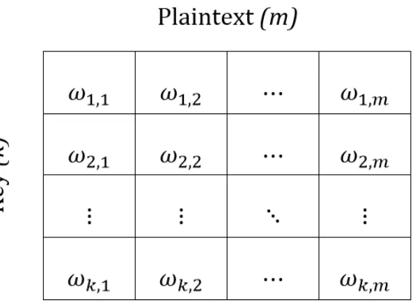
To test these models and to better visualize the testing that occurs, Figure 7 is shown to represent

the compression of an array to a 𝑘×𝑚 matrix, where each cell 𝑘,𝑚 contains the total number of

“1”s, denoted as 𝜔!,!  , that are present in that particular sequence of n bits.

Then for each of the aforementioned models, the corresponding tests, (where failure of any

single test demonstrates non-randomness) are:

1. Test 1: Apply one standard binomial test to the entire 𝑘×𝑚 matrix

2. Test 2: Apply k (or m) binomial tests to each row (or column) in the matrix

3. Test 3: Apply kmbinomial tests to each individual cell in the matrix

It is important to note that because Test 2 and Test 3 exercise multiple testing, the Sidak

corrections for multiple comparisons as previously described are required. Also, as formerly

mentioned, the discrete nature of the binomial distribution complicates the comparisons of the

tests conducted as they relate to acceptable type I errors. Because the critical values of the tests

are restricted to integers, it is the case that the exact 𝛼! cannot be obtained in some cases. To

alleviate this, the normal approximation to the binomial distribution is applied, which then

allows for all real critical values, and thus an exact 𝛼!. Here, the power of each individual

binomial test can be approximated by:

1−Φ Δ+𝑐

𝜎 +Φ Δ−

𝑐

𝜎

where

Δ=𝑝!−𝑝

𝜎 ,      𝑐 =−𝜎!∙Φ!!

𝛼_!

2  

and

𝜎!=

𝑝_! 1−𝑝_!

𝑛 ,      𝜎=

𝑝 1−𝑝

which allows for more thorough comparisons of the tests.

As an example, the following analytical results of these three tests are provided with k =

100, m = 100, n = 64, p0 = 0.5 and an acceptable type I error rate of 𝛼!=0.05. That is, our array

will consist of 10,000 sequences of 64 bits obtained from the encryption of 100 different

plaintexts by 100 different keys. It is assumed that the probability of “1” occurring in the

sequence is 0.5. This allows us to demonstrate how the power of the binomial tests differ from

test to test as well as practical applications in a computer science setting.

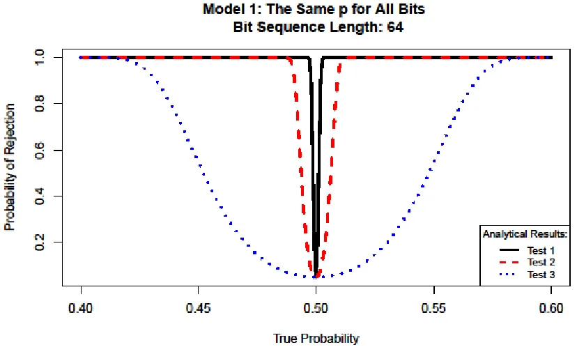
Figure 8: Power of tests applied to Model 1

It is clear from the graph that when Model 1 is evaluated, Test 1 is the most powerful of the three.

This is evident because with only slight change in true probability from 𝑝=0.5, Test 1 will make a

proper rejection. Test 2 does not perform as well as Test 1, however, it does not take much more change

not perform very well at all. It takes more than ±0.075 change in true probability before the test will

consistently make the correct rejection. These results are as expected since detection for this particular

model is truly dependent on the vast differences of the sample sizes of the tests.

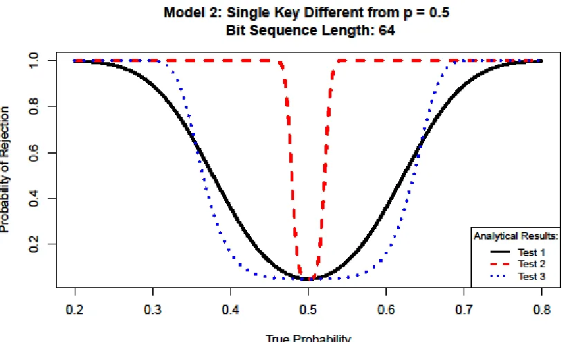
Figure 9: Power of tests applied to Model 2

For Model 2, in the event that we have a week key supplying bit sequences with 𝑝≠0.5,

the test that will best make a detection is Test 2. We can see that the test will make the detection

in cases with the least variation from 𝑝=0.5 of the three. This is also as we would expect

because this testing is conducted on rows in our array-based testing structure represented by

keys. This allows us to make the distinction between keys that perform well and those that do

not. The other tests are not designed in such a way and the detection capabilities are clearly at a

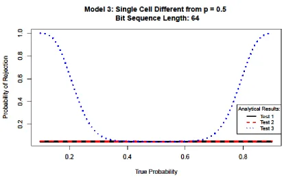
Figure 10: Power of tests applied to Model 3

Finally, when a particular plaintext/key combination produces a ciphertext with 𝑝≠0.5,

as is the case in Model 3, Test 3 is the only test that can sufficiently make the detection.

However, the detection is only consistently made when the change from 𝑝=0.5 is around ±0.3.

With a requirement for the difference from  𝑝=0.5 at such a large level, this test is the least

powerful of those required to make meaningful detections of all the models. Although, it is a

necessary test for this particular model since Test 1 and Test 2 are incapable of making any

significant detections.

It is apparent from the results that each individual test has capabilities that correspond to

the respective models. In a case where it is unknown which model may underlie within the

array-based testing structure, all three tests should be conducted to improve the chances for identifying

presentation of tests was done using arbitrarily selected values for k, m, n, and p0. These

parameters can easily be changed to meet the needs of those interested in conducting tests with

this structure. In fact, as is known, increasing the sample size for the tests results in more

powerful testing for these models. This will be demonstrated more in-depth with comparisons of

simulated data. However, with more powerful testing comes the trade-off for computational

time, and this is something that needs to be investigated prior to establishing this array-based

8. Simulated Results

for Array

-based Tests

To further assess these analytical results and attempt to tie these principles to practical

application, we create simulations of the binomial data that follow the arrangements of the three

models investigated. In order to begin, we determine an acceptable precision for the simulations,

and in turn, an acceptable replication size. Since the standard error of the proportion is:

𝑆𝐸_!"#!#"$%#&=   𝜃 1−𝜃

𝑁

where 𝜃 is the proportion presented and N is the replication size, the margin of error, with 95%

confidence, for the worst case, when 𝜃=0.5 is demonstrated in the

following figure.

For this worst case, we can obtain a precision of ±0.02 with 2500 replications. If

precision of ±0.02 is considered acceptable at this level, (which with computing time in

consideration, we will), simulations will be presented with 𝑁=2500.

For Model 1, we simulate the power of the tests for k = 100, m = 100, n = 64, comparing

the values of p = 0.480, 0.485, 0.490, 0.495, 0.500, 0.505, 0.510, 0.515, 0.520 to those acquired

analytically. The following figure demonstrates this comparison.

Figure 12: Comparison of analytical and simulated results for Model 1, 64-bits

What is clear from the results of the simulation for Model 1 is that although Test 1 and

Test 2 appear to demonstrate similar values for the corresponding analytical results, Test 3 does

not appear to perform as expected. In fact, the simulated power values for Test 3 are consistently

simulation criteria, the 95% CI error bars surrounding the simulated values do not contain the

analytical results calculated by the normal-approximation to the binomial.

Figure 13: Test 3 Simulation errors and analytical results for Model 1

This is a pattern that is also evident with k = 100, m = 100, n = 64 in the simulations for

Model 2 where p = 0.30, 0.35, 0.40, 0.45, 0.50, 0.55, 0.60, 0.65, 0.70 and Model 3 where p = 0.1,

0.2, 0.3, 0.4, 0.5, 0.6, 0.7, 0.8, 0.9, shown in figures 14 and 15 respectively, at least with values

Figure 14: Comparison of analytical and simulated results for Model 2, 64-bits

Figure 16: Test 3 simulation errors and analytical results for Model 2

Since Sidak corrections for multiple testing were utilized with 𝛼_! =0.05, it is expected

that both our analytical and simulated results coincide for p = 0.5 at a probability of rejection

𝛼_!= 0.05. That is, in our example of 2500 replications, if the 10,000 bit sequences, each of

length 64, actually were generated with a true probability of 0.5 for the “1”s in each bit sequence,

we would expect that at least 1 test, within that family of 10,000 tests, to incorrectly fail at a

theoretical rate of 0.05 (or 125 of the 2500 replications). For Test 1 and Test 2, this appears to be

the case. However, Test 3 consistently fails at a much lower rate. This result brings about the

question of how much the discreteness and bit-length of the sequence play in the role in properly

9. Investigations

of

Discreteness and Bit

-

length for Binomial Testing

As previously discussed in chapter 7, the discreteness of the bit sequences in the three

binomial test applications led to the utilization of normal-approximation to the binomial for the

calculations of our analytical results. For Test 1 and Test 2, these results appeared to agree with

the simulated results. However, for Test 3 this was not the case. For simulations, across all

models, we consistently witnessed simulated values significantly lower than those values which

we were able to acquire analytically. In one regard, we have an interest in demonstrating that this

can be attributed solely to the discreteness of the data. That is, critical values can only take on

integers and therefore there is a finite set of possible values which our test statistic can take on.

When we increase the bit-length, we provide more opportunities for critical values to take on

integers below or above our confidence level. Without diving too deep into the underlying

distribution, this assumption would explain the reason that Test 1 and Test 2 perform correctly,

while Test 3 underperforms in practice. However, this is not at all the case.

To better understand what is going on, we further investigate Test 1, Test 2, and Test 3 at

p = 0.5, for n = 32, 33, …, 300. We can view the probability of rejection from the exact binomial

test at p = 0.5, because we know that across all tests, we expect the probability of rejection to be

0.05, which is exactly what we were able to demonstrate analytically. However, we know that

because the binomial test is discrete, the probability of rejection will most likely not be an exact

match. So we have two options for comparison. We can select a critical value a, such that:

1. 𝑀𝑖𝑛 𝑃 𝑋<𝑎 −𝛼! ₂

In Figure 18 we can see the probability of rejection using option 1. Also, n = 64, 128, and

256 are highlighted with boxes to demonstrate their connection to bit-length in computer science.

In Figure 19 we can see the probability of rejection using option 2. Again, n = 64, 128, and

256 are highlighted with boxes.

From Figure 18, we can see that the exact binomial calculations, at n = 64 for both Test 1

and Test 2, are values that compare nicely with our analytical power value of 0.05. These values

are so close to our analytical value that it appears that these calculations could demonstrate our

simulated results from chapter 8. However unlike our simulations, the power for Test 3 is near

0.07, which was not at all the case with our simulated values.

In Figure 19, again we can see that the exact binomial calculations, at n = 64 for both Test

1 and Test 2, appear to be values close to what were acquired through simulations and values that

are close to our analytical results. However for Test 3, at n = 64 we see a value that is

significantly lower than our analytical power value of 0.05. This mirrors the results that we

obtained from the simulations in chapter 8 and explains why our simulations appeared so low for

Test 3 since the underlying method of our simulations used the principles of option 2.

To tie these options into practical applications, it is important to remember that we first

mentioned acceptable errors in chapter 2, and that throughout this paper we have been

demonstrating results based on 𝛼_!= 0.05. The importance lies with what we can truly proclaim

our confidence to be. At the 𝛼_! =0.05 level we can be 95% confident in our results.

Importantly, we make initial acceptance that we will wrongly reject H0 at the 𝛼!= 0.05 level

and that is something which our results must reflect. More importantly, if we make this claim

and we demonstrate results at or less than this level, we are still correct and are not falsely

providing evidence for our case. It is when our findings do not support our claim that we

contradict ourselves. This is demonstrated in these two options and is especially evident in

Exact Binomial

Value at p = 0.5 Absolute Difference from 𝛼_! = 0.05

Option 1 0.06825409 0.01825409

Option 2 0.018633842 0.03136616

Table 1: Comparison of option 1 and option 2 for 64-bits

From Table 1, we can see that the exact binomial value for option 1 is 0.06825409, while

option 2 is 0.018633842. This means that technically using option 1 gives a value that is closer to

our analytical result of 0.05 (absolute difference of 0.01825409) compared to option 2 (absolute

difference of 0.03136616). However, if we want to back up our claim that we are willing to

accept 𝛼_!= 0.05, our evidence is flawed in reporting values using option 1. We are only truly

correct if at p = 0.5 we can show values at or below 𝛼_! =0.05, and this will always be the case

with option 2. For this reason, option 2 is the best method for providing results from discrete

distributions. This is also the reason that simulations were calculated in the same manner.

As for the role of bit-length, it is clear that there is convergence to a power value of 0.05

at p = 0.5 for Test 3 in both option 1 and 2. This is shown in Figure 20 and Figure 21

respectively, where again p = 0.5, but in an effort to save computational time n = 100, 200, 300,

Figure 20: Exact binomial power calculations, Test 3, option 1

However, this is unrealistic in a computer science setting. Ciphertexts from encryption

algorithms do not require bit sequences of such massive length, nor would they be viable.

Therefore, we can see that the least powerful of these tests is indeed Test 3. In a general sense,

increases of the bit-length will make overall trend of the test more powerful, but the local

variation resulting from these increases does not technically allow for us to improve this power

10. Conclusion and Future

Applications

In this thesis, we investigated many nuances of statistical randomness testing applicable

to the field of computer science. This project initially began as a statistical investigation of the

Coincidence Test and the way in which testing errors within the test are produced. This quickly

led us to examining the potential for an array-based testing structure. We were able to determine

that there are indeed benefits to using such a structure, but with these benefits also comes

complications, which is something that needs to be understood prior to any implementation.

First, we understand that computing storage is a main drawback to this technique. There

are too many combinations of plaintexts and keys to store all possible outcomes from

encryptions. Therefore we recommend creating this test array using random subsets of plaintexts

and keys which are feasible to encrypt and store. The main benefit for this structure is that there

is no requirement for all possible ciphertexts to gain valuable insight on the encryption function.

Using these random subsets will suffice, as long as all combinations of the selected subset are

captured. Obviously, the more data that can be analyzed the better the test will be, but the storage

of these ciphertexts must be taken into consideration and simply adding another key the array

can quickly add thousands and thousands of bits that must be properly stored.

Secondly, we understand that as this type of testing applies to computer science, the tests

will be conducted on discrete data. Therefore when deciding a confidence level for the test,

careful consideration must be made regarding the determination of significance and critical

values. As shown in Chapter 9, there is importance in deciding significance and using proper

Lastly, we reported the results of our array-based testing structure using the three testing

options (Test 1, Test 2 and Test 3) of the binomial test. Though this is a crucial test, and is one

that is often used, this testing structure is capable of so much more. Essentially, any statistical

test which used entire strings of bits can benefit from this structure. For example, the same

process described in this paper can be applied to the Wald-Wolfowitz runs test [4], to determine if

the exchange from “0” to “1” (or “1” to “0”) within the string occurs more or less often than

expected. The limit is only on the number of relevant tests available.

Creating a collection of these types of tests and applying them to the array-based

structure can assist in validating the underlying encryption function, not only the encryption

output, which again is beneficial in understanding the encryption process. At the end of the day,

this is of the most importance and this testing structure should be added to the arsenal of other

Bibliography

[1] Kaminsky, Alan. The Coincidence Test: a Bayesian Statistical Test for Block Ciphers and

MACs (2013). http://www.cs.rit.edu/ ark/parallelcrypto/cryptostat/coincidence.pdf

[2] Ferguson, Niels, and Bruce Schneier. Practical Cryptography (1 ed.). New York: John Wiley

& Sons, Inc., 2003 (6 – 22).

[3] Lawrence E. Bassham, III, Andrew L. Rukhin, Juan Soto, James R. Nechvatal, Miles E.

Smid, Elaine B. Barker, Stefan D. Leigh, Mark Levenson, Mark Vangel, David L. Banks,

Nathanael Alan Heckert, James F. Dray, San Vo, SP 800-22 Rev. 1a. A Statistical Test

Suite for Random and Pseudorandom Number Generators for Cryptographic

Applications, National Institute of Standards & Technology, Gaithersburg, MD, 2010.

[4] Wolfowitz J. (1943). On the theory of runs with some applications to quality control, The

Annals of Mathematical Statistics 14, 280–288.