Econometric modelling of multiple self-reports of
health states: The switch from EQ-5D-3L to EQ-5D-5L
in evaluating drug therapies for rheumatoid arthritis
M´
onica Hern´
andez-Alava
Stephen Pudney
School of Health and Related Research, University of Sheffield
This version June 14, 2017
Abstract
EQ-5D is used in cost-effectiveness studies underlying many important health policy deci-sions. It comprises a survey instrument describing health states across five domains, and a system of utility values for each state. The original 3-level version of EQ-5D is being replaced with a more sensitive 5-level version but the consequences of this change are uncertain. We develop a multi-equation ordinal response model incorporating a copula specification with normal mixture marginals to analyse joint responses to EQ-5D-3L and EQ-5D-5L in a sur-vey of people with rheumatic disease, and use it to generate mappings between the alter-native descriptive systems. We revisit a major cost-effectiveness study of drug therapies for rheumatoid arthritis, mapping the original EQ-5D-3L measure onto a 5L valuation basis. Working within a comprehensive, flexible econometric framework, we find that use of sim-pler restricted specifications can make very large changes to cost-effectiveness estimates with serious implications for decision-making.
Keywords: EQ-5D, ordinal response, copula, mixture models, rheumatoid arthritis, map-ping, cost-effectiveness
JEL codes: C35, C83, D61, H51, I10
Contact: Steve Pudney, ScHARR, University of Sheffield, Regent Court, 30 Regent Street, Sheffield, S1 4DA, UK; tel. +44(0)114 2229187; email: steve.pudney@sheffield.ac.uk
1
Introduction: EQ-5D-3L and EQ-5D-5L
The quality-adjusted life year (QALY) is one of the most widely used health benefit
mea-sures in economic evaluations of interventions, services or programmes designed to improve
health. The QALY reflects concerns for both quality and length of life and allows health
care decision makers to use a consistent approach across a broad range of disease areas,
treatments, and patients. QALY estimation is based on patient-reported outcome measures
(PROMs), of which EQ-5D is a leading example. EQ-5D is recommended by the English
National Institute for Health and Care Excellence (NICE) for its technology appraisals, but
it has wider international significance: public bodies in at least ten other countries also
recommend EQ-5D as a basis for cost-effectiveness analysis.1 It is also increasingly used as
a measure of performance in wider economic contexts, and as a generic health measure in
population surveys (Devlin and Brooks, 2017). There is continuing debate about the basis
of economic appraisal in health policy, with interest in wider outcome measures based on
wellbeing or capabilities, income-variation valuations, and the use of weights for different
aspects of disease such as burden of disease or rarity (Brazier and Tsuchiya, 2015).
Never-theless, for the foreseeable future, it seems inevitable that cost per QALY will continue to
be the main driver of decisions in many public health services around the world.
EQ-5D measures patient outcomes across five dimensions: mobility, self-care, usual
ac-tivities, pain/discomfort, and anxiety/depression. The original version of EQ-5D, which has
been used in a large number of cost-effectiveness evaluations, measures each domain on a
scale with three severity levels (no problems, some or moderate problems, extreme problems).
Up to 35 =243 states of health can be described in this way, and each has been assigned a
utility score on the basis of an analysis of preferences over length and quality of life using
1Including Belgium, Colombia, Egypt, Estonia, Ireland, Latvia, Lithuania, the Netherlands, New Zealand
data from the general public (Dolan, 1997); full health is assigned a utility score of 1, 0 is
equivalent to death, and negative values indicate health states worse than death.
Concerns about (lack of) sensitivity and floor/ceiling effects in the standard version
re-cently led to the development of a new version, the EQ-5D-5L. The descriptive system covers
the same five dimensions but the number of levels within each dimension has been extended
from three to five (no problems, slight problems, moderate problems, severe problems,
ex-treme problems). In addition, some of the wording has been modified to aid consistency and
understanding.2 The maximum number of health states that can be described with the new
version is 55 =3125. Several studies have reported better measurement properties in moving
from the EQ-5D-3L to EQ-5D-5L in both specific patient and general population samples
(Pickard et al., 2007; Janssen et al., 2013; Scalone et al., 2013; Agborsangaya et al., 2014;
Jia et al., 2014). Utility value sets for EQ5D-5L have been proposed for England (Devlin
et al., 2016), Japan (Ikeda et al., 2015), Canada (Xie et al., 2016), Uruguay (Augustovski
et al., 2016), Netherlands (Versteegh et al., 2016) and Korea (Kim et al., 2016) and similar
work is underway in many other countries. Many studies now include EQ-5D-5L instead of
the standard version. Since these studies will form part of the evidence in future economic
evaluations, it is important to assess the likely consequences for economic evaluation
deci-sions of moving across the two different verdeci-sions of EQ-5D, and to develop a basis for using
the very large stock of existing evidence based on the 3L version.
If both variants of the EQ-5D instrument are observed in the same dataset and a utility
score is available for each, it is possible to use a conditional statistical model to map directly
from the 3L utility score to the 5L score or vice versa. However, that direct approach has
three major disadvantages. First, utility scores have highly irregular empirical distributions
and the most widely used mapping methods often fit poorly (Hern´andez-Alava et al., 2012).
2See the EuroQol website
Second, use of a single utility score to summarise the 5-dimensional observed response fails
to exploit all of the information contained in the observed EQ-5D responses. Third, the
di-rect approach is necessarily specific to the particular scoring system used to construct utility
values for the 3L and 5L health descriptions, making it hard to explore sensitivity to
varia-tions in the choice of scoring system. The alternative approach known as ‘response mapping’
(Gray et al., 2006) models the statistical relationhip between the 3L and 5L responses and
only brings utility scoring in at the final stage. By separating the logically distinct
compo-nents of health state measurement and utility scoring, response mapping gives (in our view)
a more natural way to proceed.
Although statistical mapping is often treated as a routine and arcane statistical task, it
can have a critical impact on the outcome of economic decision-making, and the
economet-ric assumptions used for mapping between alternative PROMs need to be examined very
carefully. Those assumptions include: the choice of covariates for the mapping model,
distri-butional specification, and independence or dependence of responses across the five domains
of EQ-5D. Various statistical specifications appear in the small existing literature. Some
au-thors have assumed conditional independence between the five domains of EQ-5D, estimating
a separate model for each domain. Using this approach, van Hout et al. (2012) developed
a mapping between EQ-5D-3L and EQ-5D-5L to construct an interim scoring system for
EQ-5D-5L derived from the Dolan (1997) scores for EQ-5D-3L. However, independence is
an implausible assumption: medical conditions may simultaneously affect multiple aspects
of life – for instance severe pain may be accompanied by depression and curtailment of
ac-tivities. Also, there may be individual-specific styles of questionnaire response which affect
responses in all domains – some people tend to look on the bright side, while others do not.
The conventional normality assumption built into the univariate or multivariate ordered
pro-bit model is also a strong one, and consistent estimation is not achieved in general if error
In section 3 of the paper, we develop a multi-equation model that allows for the discrete
EQ-5D response scales and uses a flexible mixture-copula specification of the error
distri-butions. Importantly, we do not impose the assumption that responses in the five domains
of EQ-5D are statistically independent. In section 4, we apply the model to investigate the
consistency of the responses to the two descriptive systems and the implied differences in the
utility values. We derive the appropriate mapping technique in section 5 and compare the
results from mapping in both directions between the two variants of the EQ-5D instrument.
To explore the implications of modelling strategy for real-world policy decisions, we report
an application to cost-effectiveness of treatments for rheumatoid arthritis (RA). We focus on
RA partly for its inherent importance – among the 291 medical conditions covered by the 2010
Global Burden of Disease Study (Murray, 2012), RA ranked as the 42nd greatest contributor
to global disability, measured in Years Lived with Disability (YLD), ranking immediately
after malaria. It is also a rapidly growing problem; between 1990 and 2010, the estimated
global burden of RA (adjusted for population growth and ageing) grew 15% in terms of YLD
and 44% in terms of disability-adjusted life years (Cross et al., 2014). But data availability
is another advantage; we have access to the National Data Bank for Rheumatic Diseases
(NDB), which provides a unique RA-specific reference dataset that observes both versions of
EQ-5D and also contains detailed clinical outcome measures. This allows us to explore one
of the most important features of the mapping process, by varying the information provided
by the covariates of the mapping model.
In section 6, we re-visit the important CARDERA cost-effectiveness study (Choy et al.,
2008; Wailoo et al., 2014) comparing four drug therapies for RA. We use statistical mapping
to convert EQ-5D-3L responses into EQ-5D-5L QALYs, and find a large impact of the choice
of statistical assumptions on the evaluation results. Our evidence suggests that the potential
raise questions about some past decisions. We begin in section 2 by describing the NDB data
that we use for the EQ-5D-3L and EQ-5D-5L comparison – one of the few datasets available
in which both variants of the instrument are carried in the same questionnaire.
2
The NDB dataset
The NDB is a register of patients with rheumatoid disease, primarily recruited by referral
from US and Canadian rheumatologists. Information supplied by participants is validated by
direct reference to records held by hospitals and physicians.3 Full details of the recruitment
process are given by Wolfe and Michaud (2011). The EQ-5D responses and other
patient-supplied data are collected by various means, primarily postal and web-based questionnaires
completed directly by patients. Data collection began in 1998 and continues to the present,
in waves administered in January and July of each year. In 2011, there was a switch from 3L
to the 5L version of EQ-5D and both versions were collected in parallel during the January
2011 wave, to allow the effects of the switch to be accommodated in analyses spanning the
whole period. Our principal aim is to use data from that wave of the survey to estimate a
joint model of the 3- and 5L responses, which can then be used to map from 3- to 5L EQ-5D
during the pre-2011 period and from 5- to 3L EQ-5D after January 2011. It then becomes
possible to investigate the consistency of the two versions of EQ-5D and assess the impact
of mapping between them.
2.1
EQ-5D response distributions
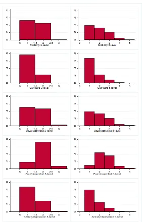
Figure 1 shows histograms of the NDB sample response distributions for the 3- and 5L
versions of each domain of EQ-5D. There are clear differences between the distributional
shapes for different domains: self-care and anxiety/depression have a dominant mode at the
first category; the mobility and usual activities domains also have a decreasing profile but
with a heavier central section, while the pain/discomfort domain shows a strong mode in
the centre of the distribution. This variation in the shape of the component distributions
underlines the need to use a suitably flexible model specification to analyse the relationship
[image:7.612.164.445.247.687.2]between variants of EQ-5D.
2.2
Utility scores
For each possible combination of EQ-5D responses, there is a utility value which allows
overall health-related quality of life to be estimated and compared across individuals and
conditions. We use the value sets produced by Dolan (1997) and Devlin et al. (2016) for the
3- and 5L versions of the instrument which, at present, are the standard choices for QALY
measurement in England. Dolan (1997) used data from a representative sample of the UK
population (2,977 respondents). Each respondent valued 13 hypothetical health states using
the time trade-off (TTO) method, generating valuations for a subsample of 42 of the 243
health states described by the EQ-5D-3L. The data were then modelled using regression
methods to impute utility values for the remaining health states. Devlin et al. (2016) used
a sample of the English population (996 respondents) who valued ten health states using a
composite TTO approach, and seven paired comparisons of health states via discrete choice
experiment tasks. The model selected for the EQ-5D-5L value set for England was a hybrid
model using both sets of data (Feng et al., 2016).
Figure 2 shows kernel density estimates of the distributions of utility scores in the NDB
data, aggregated across all five domains. The distribution is smoother for the 5L version,
particularly towards the top of the range, and this finer structure is a major reason for its
adoption in practice. The distribution of utility scores for the 3L version of EQ-5D has
two particularly worrying features. There are ranges with probability mass at or close to
zero, particularly around 0.8-1.0 and 0.3-0.45. Consequently, methods for mapping to and
from EQ-5D-3L which implicitly assume a smooth positive density can give very poor results
(Hern´andez-Alava et al., 2012). The second striking feature of the distribution for EQ-5D-3L
is the large group of cases with utility values close to zero, implying that a non-negligible
proportion of patients with rheumatoid arthritis (RA) are in a state comparable to, or worse
improve quality of life for patients in very poor health, so the (perhaps implausibly) large
[image:9.612.107.512.174.476.2]frequency of such cases is a potential source of bias in NICE recommendations.
Figure 2: Smoothed empirical distributions of EQ-5D-3L and EQ-5D-5L (Jan 2011 wave of NDB, n=5192)
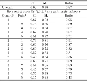
Table 1 summarises the January 2011 NDB data on the value scores for the two variants of
EQ-5D in terms of their correlation with each other, with basic demographic characteristics,
and with a set of clinical outcome measures. We use the Spearman rank correlation to show
the strength of monotonic, not necessarily linear, associations, but the Pearson correlation
shows a similar picture. There is a high correlation between the two variants of EQ-5D,
but the 5L version has greater sensitivity, since correlations with demographics and clinical
outcomes (in the lower panels of Table 1) are uniformly higher for EQ-5D-5L.
Table 2 shows that there is a systematic difference in the 3L and 5L utility scores, with
Table 1: Spearman correlations of 3- and 5L EQ-5D (Jan 2011 wave of NDB, n=4856)
Variable EQ-5D-3L EQ-5D-5L
EQ-5D-3L 1.000 0.845
EQ-5D-5L 0.845 1.000
Female -0.054 -0.074
Age 0.030 0.060
HAQ score (0-3) -0.735 -0.758
Pain scale (0-10) -0.707 -0.704
Overall RADAI score -0.737 -0.746
Global severity (0-10) -0.698 -0.721
Disease duration (months) -0.057 -0.063
Fatigue scale (0-10) -0.633 -0.669
Sleep disturbance scale (0-10) -0.506 -0.541
Arthritis activity (general) -0.611 -0.626
Arthritis activity (today) -0.672 -0.673
RADAI joints (score) -0.641 -0.648
RADAI joints (count) -0.581 -0.589
Morning stiffness (0-6) -0.538 -0.554
Co-morbidity index (0-9) -0.344 -0.360
Physical component score (SF-6D) 0.727 0.700
Mental component score (SF-6D) 0.475 0.569
Health satisfaction (0-4) -0.638 -0.671
given by the new system. This alone could make a significant difference to some evaluation
results. It would be inadvisible to address the issue with a simple proportional adjustment,
since the ratio of mean scores is not constant but decreases as both general severity and
pain increase, so the differences are minor at the top end of EQ-5D and much larger at the
bottom. Table 2 gives means classified by levels of general disability (in three groups, scores
0-1, 1-2 and 2-3) and pain (in five groups 0-2, 2-4, 4-6, 6-8 and 8-10), as classified by the
Stanford Health Assessment Questionnaire (HAQ). The HAQ is widely used by clinicians to
measure treatment outcomes; see Bruce and Fries (2003) for a review.
Mapping from 3L to 5L involves two changes: a shift from the 3L health descriptive system
to the 5L system, made using a predictive statistical mapping model; and a shift from the
Table 2: Means of EQ-5D-3L and EQ-5D-5L utility scores by severity of condition (Jan 2011 wave of NDB, n=5192)
3L 5L Ratio
Overall 0.68 0.78 0.87
By general severity (HAQ) and pain scale category
General1 Pain2 3L 5L Ratio
1 1 0.87 0.92 0.95
1 2 0.76 0.86 0.89
1 3 0.72 0.83 0.87
1 4 0.67 0.78 0.87
1 5 0.51 0.72 0.71
2 1 0.74 0.81 0.91
2 2 0.66 0.76 0.87
2 3 0.60 0.73 0.82
2 4 0.52 0.64 0.81
2 5 0.30 0.53 0.56
3 1 0.63 0.71 0.89
3 2 0.54 0.65 0.83
3 3 0.45 0.57 0.79
3 4 0.35 0.48 0.73
3 5 0.15 0.35 0.43
1Groups corresponding to HAQ scores (1) [0-1); (2) [1-2) and (3) [2-3]
2Groups corresponding to pain scores (1) [0-2); (2) [2-4); (3) [4-6); (4) [6-8) and (5) [8-10]
changes occur jointly, so it is not possible to disentangle fully the effect on cost-effectiveness
calculations of mapping from the effect of the change in utility structure. However, within a
fixed framework dictated by the given 3L and 5L utility tariffs, it is possible to compare the
results produced by alternative specifications of the mapping model. This is our strategy,
implemented within a comprehensive and flexible econometric approach.
3
A correlated copula model with mixture marginals
Our aim is to develop an econometric model of responses to the ten items of the 3L and 5L
instruments. The specification is guided by six important considerations, intended to avoid
(i) Treat the 3L and 5L responses symmetrically so that it can be used for 3L→5L and
5L→3L mapping in a mutually consistent way.
(ii) Avoid the assumption that the 5L response scale is simply a more detailed categorisation
than the 3L scale of the same underlying concept – structural differences between the two
responses are permitted if empirically necessary.
(iii) Allow for the effects of covariates – here, age, sex and clinical outcome measures, without
assuming that they necessarily influence 3L and 5L responses in the same way.
(iv) Capture the strong association between 3L and 5L responses within each health domain,
without necessarily assuming that the strength of the association is the same in all parts of
the health distribution – for example, someone who has experienced extreme pain may answer
the pain questions in a more focused and coherent way than someone without experience
of chronic pain. To achieve this, we use a copula approach (Trivedi and Zimmer, 2005) to
specify the bivariate distribution of each 3L, 5L pair of responses.
(v) Be sufficiently flexible to fit the diverse response patterns shown in Figure 1, so we
generalise the usual assumption of normally-distributed errors by allowing for a 2-part normal
mixture distribution, which can capture a wide range of distributional shapes.
(vi) Allow dependence across the five domains of EQ-5D, reflecting common underlying
causes and individual-specific response styles; we achieve this by incorporating a random
latent factor influencing responses in all domains.
In advance of the empirical analysis, there is no way of knowing which of these
considera-tions is most important, so the resulting model is complex. Define 1≤Y3id≤3 and 1≤Y5id≤5
as the reported outcomes for the dth domain (d=1. . .5) of the 3- and 5L forms of EQ-5D.
domaind containing the equations for Y3id and Y5id:
Y∗
3id = Xiβ3d+U3id
Y∗
5id = Xiβ5d+U5id
⎫⎪⎪ ⎬⎪⎪ ⎭
d=1...5 (1)
where i indexes independently sampled individuals, Xi is a collection of row vectors of
covariates, β3d, β5d are corresponding coefficient vectors and U3id, U5id are unobserved errors
which may be stochastically dependent and non-normal. The latent dependent variables
Y∗
3id, Y
∗
5id are not observed directly but they have observable ordinal counterparts, Y3id, Y5id,
generated by the following threshold-crossing conditions:
Ykid=q iff Γkqd≤Ykid∗ <Γk(q+1)d; q=1...Qk; k=3,5 (2)
whereQk=3 or 5 is the number of categories of Ykid and the Γkqd are threshold parameters,
with Γk1d= −∞ and Γk(Qk+1)d= +∞.
High-dimensional ordinal-variable applications present major computational problems.
Currently, there is only a single published model of EQ-5D responses that relaxes
indepen-dence (Conigliani et al., 2015), using a 5-equation correlated multivariate ordered probit
model to predict EQ-5D responses from aggregate SF12 scores. Using that model in our
10-dimensional 3L-5L mapping context would involve estimation of 45 residual covariance
parameters, with a likelihood requiring numerical integration over a 10-dimensional rectangle.
Past experience with similar maximum simulated likelihood problems, using best-practice
simulation methods like Halton sequences, tells us that likelihood-based tests and fit
statis-tics are not robust enough for model comparisons to be reliable. The conventional ordered
probit model also involves normality assumptions that are critical to its consistency property
and which we want to relax.
Possible solutions to the dimensionality problem work by imposing structure on the joint
distribution of the latent Y∗
kid. In the copula literature, the most common approach is to
and Cooke, 2002; Panagiotelis et al., 2012). However, that is most convincing when there
is a natural ordering of the observed variables, particularly temporal sequencing (as in the
application by Panagiotelis et al. (2012) to a sequence of four observations on headache
spaced through the day). In our case, although the component items of EQ-5D-5L were
asked in sequence and then the items of EQ-5D-3L later in the questionnaire, that ordering
does not correspond at all to the natural connections between the 3L and 5L items through
their shared meaning. For that reason, we adopt a different approach, using five separate
bivariate copulas for the five domains of EQ-5D, and connecting the domains via a latent
factor V which represents common influences on the respondent’s responses. The error Ukid
is decomposed into the latent factor Vi and a specific error εkid correlated within but not
between domains:
Ukid=ψkdVi+εkid (3)
where the ψkd are a set of ten parameters. We make the standard assumptions that,
condi-tional on Xi: Vi is independent of all the εkid; the εkid are all mutually independent, except
that ε3id, ε5id are possibly dependent within any health domaind.
We use a copula representation to capture dependence between the 3L and 5L responses
for any domain. Suppressing the i subscript, define Fd(ε3d, ε5d) as the distribution function
(df) for domain d and F3d(ε3d) =Fd(ε3d,∞) and F5d(ε5d) =Fd(∞, ε5d) to be the marginals.
Their joint df for domain d is specified as:
Fd(ε3d, ε5d) =cd(G3d(ε3d), G5d(ε5d);θd) (4)
where Gkd(.) is the marginal df of εkd and θd is a parameter controlling the dependence
be-tweenε3dand ε5d. The functioncd(.)is known as a copula and, together with the marginals
G3d(.), G5d(.)it uniquely characterises the bivariate distribution of ε3d, ε5d. It has the
prop-ertiescd(0, u) =cd(u,0) =0 and cd(1, u) =cd(u,1) =ufor any 0≤u≤1 (Trivedi and Zimmer,
Gaussian: c(ε3, ε5) =Φ(Φ−1(ε3),Φ−1(ε5);θ)
where Φ(., .;θ)is the distribution function of the bivariate normal with correlation coefficient
−1≤θ≤1 and Φ−1(.) is the inverse of the univariate N(0,1) df
Clayton∶ c(ε3, ε5) =⎧⎪⎪⎨⎪⎪
⎩
[max{ε−θ
3 +ε
−θ
5 −1,0}]
−1/θ
for 0<θ≤ ∞
ε3ε5 for θ=0
F rank∶ c(ε3, ε5) =⎧⎪⎪⎨⎪⎪
⎩ −1
θln(1+
(e−θε3−1)(e−θε5−1)
e−θ−1 ) for θ≠0
ε3ε5 for θ=0
Gumbel: c(ε3, ε5) =exp(− [(−lnε3)θ+ (−lnε5)θ] 1/θ
)for θ≥1
Joe: c(ε3, ε5) =1− [(1−ε3)θ+ (1−ε5)θ− (1−ε3)θ(1−ε5)θ] 1/θ
for θ≥1
The Gaussian and Frank copulas are similar in that both allow for positive or negative
dependence, symmetric in both tails, but the Frank form generates dependence weaker in the
tails and stronger in the centre of the distribution. The Clayton copula allows only positive
dependence, with strong left tail dependence and relatively weak right tail dependence;
thus, if two variables are strongly correlated at low values but less so at high values, then
the Clayton copula is a good choice. To show the effect of copula choice, Figure 3 shows
simulated scatter plots generated using these three copulas.4 The Gumbel and Joe copulas
(not illustrated) display weak left tail dependence and strong right tail dependence, which
is stronger for the Joe than the Gumbel copula.
The within-domain specification is completed by a normal mixture assumption which
allows any of the errors εkid to have a non-normal form:
G(ε) =πΦ((ε−µ1)/σ1) + [1−π]Φ((ε−µ2)/σ2) (5)
where: 0≤π≤1 is the mixing parameter;(µ1, µ2)and(σ1, σ2 ≥0)are location and dispersion
parameters constrained to satisfy the mean and variance normalizations πµ1+ (1−π)µ2 ≡0
4Samples generated by Monte Carlo simulation, from copulas specified with Kendall’sτ
Figure 3: Pseudo-random samples drawn from three alternative copulas
0.0 0.2 0.4 0.6 0.8 1.0
0.0 0.2 0.4 0.6 0.8 1.0 Gaussian Copula
0.0 0.2 0.4 0.6 0.8 1.0
0.0 0.2 0.4 0.6 0.8 1.0 Frank Copula
0.0 0.2 0.4 0.6 0.8 1.0
0.0 0.2 0.4 0.6 0.8 1.0 Clayton Copula
andπ(σ2
1+µ21)+(1−π) (σ22+µ22) =1. These normal mixtures can capture a wide range of
dis-tributional shapes, including skewness and bimodality. The mixture (5) can be implemented
with various degrees of generality, by assuming the same parameter values (π, µ1, µ2, σ1, σ2)
for all error terms, or allowing them to vary with domain d = 1...5 and/or EQ-5D design
k=3,5. We specify a normal mixture distribution for the latent factor V also.
Conditional on X, the probability of observing any values Y3d=q and Y5d=r is:
P (q, r∣X, d) = cd(Gkd(q+1), Gkd(r+1)) −cd(Gkd(q+1), Gkd(r))
−cd(Gkd(q), Gkd(r+1)) +cd(Gkd(q), Gkd(r)) (6)
where Gkd denotesGkd(Γkqd−Xβkd). The joint distribution of Y31, Y51. . . Y35, Y55 is:
P r(Y31, Y51. . . Y35, Y55∣X) = ∫ 5
∏
d=1
P(Y3d, Y5d∣X, v) [
p s1
φ(v−m1 s1 ) +
1−p s2
φ(v−m2 s2 )]
dv
(7)
We use Gauss-Hermite quadrature with 15 integration points to evaluate the integral in (7)
4
Modelling results
Our aim is to estimate the joint distribution of the responses to the 3L and 5L variants of
the EQ-5D survey instrument, conditional on demographic characteristics (age and gender),
and clinical measures of the severity of the underlying rheumatic condition. We use seven
covariates: age, gender, the HAQ disability score, the pain scale, and the squares and product
of the HAQ and pain scales.
The HAQ is based on patient self-reporting of the degree of difficulty experienced over the
previous week in eight categories: dressing and grooming, arising, eating, walking, hygiene,
reach, grip, and common daily activities. It is widely used by clinicians to measure health
outcomes. It is scored in increments of 0.125 between 0 and 3 (although it is standard to
consider it fully continuous), with higher scores representing greater degrees of functional
disability. The HAQ instrument also includes separately a patient self-report of pain scored
on a Visual Analogue Scale (0-10).
4.1
Domain-specific modelling
We start by examining each of the five domains of EQ-5D separately using a bivariate
approach, implemented in the Hern´andez-Alava and Pudney (2016) Stata bicop routine.
There are several reason for this: it is computationally easier to make the choice of copula
for each domain separately, and the process generates good parameter starting values for
likelihood optimisation for the full model. Also, although conditional independence between
domains is rather implausible, if independence is not rejected, or if it turns out to have
little adverse impact on cost-effectiveness applications, then domain-specific modelling offers
Table 3 summarises the sample fit of alternative copula functions for the 3L- and 5L
variants for each of the five domains, where we retain the standard assumption of Gaussian
marginals. There is no single best choice of copula: the Gaussian form fits best for dimensions
1 and 3 (mobility and usual activities), the Frank copula fits best for dimensions 2 and 5
(self-care and anxiety/depression) while the Gumbel copula fits best for the pain/discomfort
dimension. This coincides with differences in the empirical distributions of Figure 1 between
these three groups of domains. The Frank copula (which allows weaker dependence in the
tails than the centre of the distribution) works better than the Gaussian copula when the tails
of the response distribution are relatively heavy. The Gumbel copula which has asymmetric
dependence in the tails (stronger dependence at higher values) fits better when there is a
central mode and implies different patterns of dependence in both tails of the distribution.
Table 3 also gives the results of the Wald test of the null hypothesis that the coefficient
vectors relating the (latent) response to age, gender and disease severity are identical in the
3- and 5L variants. The hypothesis is clearly rejected for the domains of mobility and pain.
This finding shows that the effect of the move to 5 levels is not simply a uniform re-alignment
of the response level.5
The assumption of normal marginals for the errors εkd was acceptable in terms of the
Akaike (AIC) and Bayesian (BIC) information criteria for the mobility, self-care and
anxi-ety/depression domains, but there was significant evidence of modest departures from
nor-mality for the usual activities and pain/discomfort domains. Table 4 summarises the
pre-ferred specifications for those two domains, comparing them with the simpler
Gaussian-marginal models. Note that the conclusions about the equality of coefficients are not affected
by non-normality.
5Note that these are formally tests of the hypothesis that the coefficient vectors are equal after each error
Table 3: Sample fit of domain-specific models for alternative copula functions with Gaussian marginals)
Copula
Gaussian Frank Clayton Gumbel Joe
Mobility domain
Log-likelihood -6656.54 -6665.73 -6727.46 -6669.82 -6736.73
χ2(7) for H
0 ∶β3=β5 29.02∗∗∗ 29.49∗∗∗ 23.82∗∗∗ 33.64∗∗∗ 37.14∗∗∗
Self-care domain
Log-likelihood -4221.35 -4212.35 -4248.89 § §
χ2(7) for H
0 ∶β3=β5 8.31 5.98 5.35
Usual activities domain
Log-likelihood -6772.96 -6796.04 -6866.11 -6785.64 -6829.65
χ2(7) for H
0 ∶β3=β5 10.87 10.22 10.89 11.23 11.53
Pain/discomfort domain
Log-likelihood -6148.63 -6148.07 -6190.84 -6147.80 -6199.63
χ2(7) for H
0 ∶β3=β5 29.75∗∗∗ 30.26∗∗∗ 32.71∗∗∗ 29.09∗∗∗ 26.82∗∗∗
Anxiety/depression domain
Log-likelihood -6243.59 -6238.86 -6300.55 -6244.72 -6302.70
χ2(7) for H
0 ∶β3=β5 12.05∗ 8.56 5.10 10.66 11.86
[image:19.612.80.538.426.519.2]Best-fitting models in bold type (all models have 15 parameters). Statistical significance: * = 10%, ** = 5%, *** = 1%. §No convergence.
Table 4: Estimated non-normal error distributions
Gaussian marginals Non-Gaussian marginals
Preferred Coefficient
mixture equality
Domain AIC BIC specification AIC BIC test: χ2(7)
Usual activities1 13587.9 13725.5 equal 13550.5 13707.8 8.39
Pain/discomfort2 12337.6 12475.3 unequal 12252.9 12429.9 40.91∗∗∗
Statistical significance: * = 10%, ** = 5%, *** = 1%..1 Gaussian copula.2 Gumbel copula.
Figure 4 plots the estimated distributions for the two domains where we find significant
non-normality, and compares them to the N(0,1) form. The distributions for the usual
ac-tivities domain and for the EQ-5D-5L pain/anxiety domain are similar, both with a slightly
fatter right tail of the distribution. The distribution for the EQ-5D-3L pain/anxiety
dimen-sion departs from normality with a much bigger central mode, consistent with its unique
Figure 4: Estimated error distributions for the usual activities and pain/discomfort domain
0
.1
.2
.3
.4
-3 -2 -1 0 1 2 3
Mixture N(0,1)
(a) usual activities: 3L, 5L
0
.2
.4
.6
-3 -2 -1 0 1 2 3
Mixture N(0,1)
(b) pain: 3L
0
.1
.2
.3
.4
-3 -2 -1 0 1 2 3
Mixture N(0,1)
(c) pain: 5L
4.2
Joint modelling of all domains
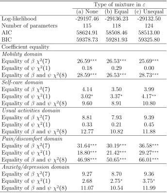
We now examine the joint model. Table 5 summarises the sample fit of alternative joint
models. All of them are based on the best fitting copulas for each dimension found in section
4.1: Gaussian for mobility and usual activities; Frank for self-care and anxiety/depression;
and Gumbel for pain/discomfort. Model (a) is the baseline model with no mixtures in ε;
model (b) allows a common mixture, constrained to be the same for the errors in all ten
equations; and model (c) allows for one common mixture for the usual activities domain and
different mixtures for the 3L and 5L equations for pain/discomfort, following the pattern
in Table 3. The joint log-likelihood, AIC and BIC for the model with independent
EQ-5D dimensions are -29958.431, 60144.86 and 60892.12 respectively, indicating that the joint
model provides a better fit to the data. The joint model with a common mixture, model
(b), gives the best fit to the data according to AIC and BIC. The conclusions about the
equality of coefficients are not affected by the choice of error distributions and are in line
with the conclusions of the domain-specific bivariate models. The estimated coefficients of
the domain-specific bivariate and joint models are shown in Appendix Table A1.
Figure 5 illustrates the effect of the differences in the distribution functions (df) of the
latent variables Y∗
ikd, evaluated at the sample mean values of the indexes Xiβˆkd. These dfs
Table 5: Sample fit of joint copula models
Type of mixture in ε
(a) None (b) Equal (c) Unequal
Log-likelihood -29197.46 -29136.23 -29132.50
Number of parameters 115 118 124
AIC 58624.91 58508.46 58513.00
BIC 59378.73 59281.93 59325.80
Coefficient equality Mobility domain
Equality of β χ2(7) 26.59∗∗∗ 26.53∗∗∗ 25.69∗∗∗
Equality of ψ χ2(1) 0.18 0.29 0.00
Equality of β and ψ χ2(8) 28.59∗∗∗ 26.53∗∗∗ 28.73∗∗∗
Self-care domain
Equality of β χ2(7) 4.14 3.50 3.99
Equality of ψ χ2(1) 3.02∗ 3.37∗ 4.17∗∗
Equality of β and ψ χ2(8) 9.60 8.91 10.80
Usual activities domain
Equality of β χ2(7) 8.81 7.93 9.39
Equality of ψ χ2(1) 0.33 0.21 0.45
Equality of β and ψ χ2(8) 12.77 10.82 11.88
Pain/discomfort domain
Equality of β χ2(7) 31.64∗∗∗ 30.19∗∗∗ 36.58∗∗∗
Equality of ψ χ2(1) 18.80∗∗∗ 21.42∗∗∗ 29.27∗∗∗
Equality of β and ψ χ2(8) 46.98∗∗∗ 50.65∗∗∗ 66.01∗∗∗
Anxiety/depression domain
Equality of β χ2(7) 9.27 8.70 9.36
Equality of ψ χ2(1) 2.68 2.75∗ 3.75∗
Equality of β and ψ χ2(8) 11.07 10.54 11.99
Statistical significance: * = 10%, ** = 5%, *** = 1%.
(to a lesser degree) usual activities domains. Moreover, the two threshold parameters for
the 3L model fall respectively between the bottom two, and top two thresholds in the 5L
model (ˆΓ52d < Γˆ32d < Γˆ53d and ˆΓ54d < Γˆ33d < Γˆ55d ), which is consistent with the idea of a
simple re-alignment of responses. However, for the mobility and pain/discomfort domains,
the differences between dfs are sizeable and statistically significant, with the pain/discomfort
domain displaying the largest difference. For both mobility and pain/discomfort, one of the
3L threshold parameters lies outside the range covered by the 5L threshold parameters, which
Figure 5: Estimated distribution functions and cutpoints forY∗
3 and Y5∗ (joint model, evaluated at covariate sample means)
0 .2 .4 .6 .8 1
-2 -1 0 1 2 3 4 5 6 7 Mobility 0 .2 .4 .6 .8 1
-2 -1 0 1 2 3 4 5 6 7 Self-care 0 .2 .4 .6 .8 1
-2 -1 0 1 2 3 4 5 6 7 Usual activities 0 .2 .4 .6 .8 1
-2 -1 0 1 2 3 4 5 6 7 Pain/discomfort 0 .2 .4 .6 .8 1 y
-3 -2 -1 0 1 2 3 4 Anxiety/depression
3-level 5-level
5
Mapping
The best method of mapping between alternative preference-based measures depends on
the nature of the cost-effectiveness study in which the measure is to be used. Suppose, for
example, that the study is to be done on the new 5L basis, but the available evidence comes
from a clinical trial in which the older EQ-5D-3L scale is measured. The key concept is the
mean QALY, which should be constructed as E{Q(υ5(Y5))}, whereE{.}is the expectation
with respect to whatever population is potentially affected by the treatment.
There are two technical issues to be considered in mapping from 3L evidence to 5L-based
evaluation. First, the form of the function, Q(.), which maps utilities into QALYs. In most
evaluation studies, the QALY calculation Q(.) is a linear function of the utilities, so that
E{Q(υ5(Y5))} =Q(E{υ5(Y5)}). In other words, we can simply predict the utility outcome
consistent) estimator of E[υ(Y5)], it will give an unbiased (consistent) evaluation of the
expected QALY.
The second issue is the choice of predictor for υ(Y5). We have argued here that a
predictor based on a full model of P r(Y5∣Y3, X) uses more information and is capable of
giving better results than the alternative approach to mapping, which attempts to model
E(υ5(Y5)∣υ3(Y3), X) directly – often using methods like linear regression which are not well
suited to the non-standard distributions involved. When using our approach, it is
im-portant to realise that the utility scales υ(.) are nonlinear functions of the vector Y, so
E(υ5(Y5)) ≠υ5(E[Y5]). We should not map the observed 3L health description Y3 into the
5L descriptive system Y5 and then apply the utility scale υ5(.). Instead, the appropriate
method is to use the model estimated from NDB data to evaluate the probability of each
possible configuration of Y5 conditional on Y3, X and use those probabilities as weights to
evaluate the conditional expectation ofυ. The conditional df of the valuation υ5 is:
P r(υ5(Y5) ≤Υ∣Y3, X) = ∑ Y5∈UΥ
P r(Y5∣Y3, X) (8)
where UΥ is the set {Y5 ∶υ5(Y5) ≤Υ} and Υ is any given constant. The mean is:
E(υ5(Y5)∣Y3, X) = ∑ Y5∈S5
υ5(Y5)P r(Y5∣Y3, X) (9)
where S5 is the set of 3125 possible values that the vector Y5 might take.6
The choice of covariates is critical here. Mapping fromY3 rather than direct observation of
υ5(Y5)introduces no bias in the calculation of mean QALYs if the conditional mean function
E(υ5(Y5)∣Y3, X) in the population represented by the reference sample used for mapping is
identical to E(υ5(Y5)∣Y3, X) in the population represented by the trial subjects. In general,
reference samples and trial samples are drawn in quite different ways, and there is always
6Hern´andez-Alava and Pudney (2017) provide a Stata command
a possibility that the statistical relationship between Y3 and Y5 could differ substantially
between the two populations, leading to mapping bias. The use of covariates can reduce this
risk by allowing for factors which might cause theY3, Y5 association to differ across samples.
Thus, even if E(υ5(Y5)∣Y3) differs between the reference and trial samples, E(υ5(Y5)∣Y3, X)
may not, for a judicious choice of covariates. We explore this in the next section.
Several authors have commented on the loss of variation induced by mapping (Brazier
et al., 2010; Longworth and Rowen, 2011; Fayers and Hays, 2014). The sample variance of
the mean predictor (9) will always be lower than the variance of the unknown true υ5(Y5),
because the modelling process can only predict variation in υ5(Y5) arising from Y3 and X,
not the other “unexplained” components of variation. In standard cases where the QALY
calculation is linear in utilities, this does not matter, since only the conditional mean of
υ5(Y5) is required. If the aim were to estimate the variance of υ5(Y5), one would not do it
by using the variance of the predictor (9); instead, the appropriate method is to calculate
directly the variance of the distribution (8), which gives a consistent estimate ofvar(υ5(Y5))
if the mapping model is correctly specified and estimated.
If we evaluate (8) and (9) at each observation Yi3, Xi, and then average over the
sam-ple, the result is a consistent estimator of the distribution of υ5(Y5) or its mean E[υ5(Y5)].
This can be done empirically for the pre-January 2011 waves of the NDB dataset and in
reverse (predicting Y3 conditional on Y5) for the post-January 2011 waves. Figure 6a uses
the set of domain-specific bivariate models (assuming independence across domains) to
com-pare the predictive df n−1∑n
i=1P r(υ5(Y5) ≤Υ∣Yi3, Xi)and the directly-observed empirical df
n−1∑n
i=11(υ3(Yi3) ≤Υ) for the Jan 2010 wave of NDB, where1(.)is the indicator function.
Figure 6b makes the reverse comparison of the predictive df for υ3(Y3)with the empirical df
of υ5(Y5) for the Jan 2012 wave. Figure 7 makes the same comparisons for the joint model
There are two striking features of Figures 6 and 7, with important implications for the
economic evaluations carried out for public bodies like NICE. First, the predictive and actual
distributions of the 5L variant of EQ-5D are similar and much smoother than the
correspond-ing distributions for the 3L variant. This is an encouragcorrespond-ing findcorrespond-ing: if a decision maker elects
to recommend the use of the new 5L instrument and associated scoring, it may be possible
to continue to use older 3L-based evidence with appropriate mapping to 5L. Second, there
is a large difference between the 3L and 5L distributions of EQ-5D scores, whether directly
observed or mapped. Utility scores tend to be systematically higher under the 5L scoring
scheme, so the df for EQ-5D-3L lies entirely to the left of the df for EQ-5D-5L. If no other
adjustment were made, this alone might be enough to change many evaluation results, in
[image:25.612.92.527.394.565.2]the absence of offsetting adjustments to the evaluation methodology.
Figure 6: Cross-mapping based on independent domain-specific bivariate models
Figure 7: Cross-mapping based on the joint model with between-domain correlation
(a) Jan 2010: 3L→5L (b) Jan 2012: 5L→3L
Table 6 shows average values of directly-measured υ3(Y3) and the prediction
E[υ5(Y5)∣Y3, X] for the 2010 wave of NDB, and of the prediction E[υ3(Y3)∣Y5, X] and
directly-measured υ5(Y5) for the 2012 wave using the joint model. Results are given for
the whole sample and subgroups defined in terms of disease severity and demographic
char-acteristics; sample standard deviations of the measured and predicted utilities are are also
shown. As expected, there are higher mean values and smaller standard deviations for the
EQ-5D-5L scores (whether predicted or directly observed) than for EQ-5D-3L, resulting from
the different scoring of poor health states by the two value sets. Another consequence of this
is the much steeper severity gradient for the mean EQ-5D-3L utilities than for EQ-5D.
There is a slight tendency for both the 3L and 5L utilities to decline over time as the
health states of those individuals who appear in both waves tend to worsen. However, the
means of predicted and directly-observed versions of each measure are remakably close both
overall and in terms of their severity and demographic profiles.
We also see the anticipated smaller standard deviations of the predicted than
importance for the evaluation described in the next section (since the criterion is based on
the mean QALY), but it would be a concern for any evaluation that aims to investigate the
distributional pattern of QALY gains within each population group. In that case, appropriate
[image:27.612.97.517.236.603.2]measures constructed from the full distribution (8) would need to be used.
Table 6: Means and standard deviations of actual and predicted (joint model) EQ-5D-3L and EQ-5D-5L by severity of condition, age and gender.
(NDB. January 2010 wave n=3877; January 2012 wave n=3911)
January 2010 January 2012
EQ-5D-3L EQ-5D-5L EQ-5D-3L EQ-5D-5L
(actual) (predicted) (predicted) (actual)
mean (SD) mean (SD) mean (SD) mean (SD)
Overall 0.70 0.79 0.69 0.78
(0.25) (0.16) (0.21) (0.19)
Severity group
Mild 0.88 0.92 0.87 0.92
(HAQ group 1, Pain group 1) (0.12) (0.04) (0.08) (0.07)
Medium 0.62 0.71 0.61 0.73
(HAQ group 2, Pain group 3) (0.15) (0.09) (0.11) (0.11)
Severe 0.12 0.38 0.12 0.30
(HAQ group 3, Pain group 5) (0.29) (0.16) (0.19) (0.23)
Female <65 0.69 0.78 0.68 0.77
(0.26) (0.17) (0.23) (0.20)
Male<65 0.71 0.80 0.67 0.77
(0.25) (0.16) (0.24) (0.21)
Female 65-79 0.71 0.79 0.69 0.79
(0.24) (0.15) (0.20) (0.18)
Male 65-79 0.73 0.82 0.73 0.83
(0.22) (0.14) (0.18) (0.14)
Female ≥80 0.65 0.76 0.66 0.76
(0.25) (0.17) (0.20) (0.18)
Male≥ 80 0.74 0.83 0.70 0.80
(0.17) (0.12) (0.17) (0.16)
6
The impact on cost-effectiveness analysis
We now use a published cost-effectiveness study to examine the potential consequences of
the economic evaluation results in Wailoo et al. (2014), which use EQ-5D-3L data collected
as part of a trial. Then we repeat the analysis using EQ-5D-5L obtained using the
map-ping models developed in this paper. Wailoo et al. (2014) estimate the cost-effectiveness of
combinations of disease-modifying anti-rheumatic drugs (DMARDs) and short-term
adminis-tration of the steroid prednisolone (PNS), using data from the 2-year CARDERA trial which
involved 467 adult patients with early active RA (less than two years of disease duration) in
a placebo-controlled factorial design. Two DMARDS were used in the trial, methotrexate
(MTX) and ciclosporin (CS). All patients received MTX, half received step-down PNS7 and
half CS, generating four treatment groups: (1) monotherapy (MTX only), (2) combination
DMARDs (MTX and CS), (3) DMARD and steroid (MTX and PNS) and (4) triple therapy
(MTX, CS and PNS). Further details of the methods and clinical effectiveness can be found
in Choy et al. (2008).
The key criterion used in cost-effectiveness analysis is the Incremental Cost-Effectiveness
Ratio (ICER), defined as the difference in costs between two different treatment strategies,
expressed as a ratio to the difference in the QALYs that they achieve. Treatments with
ICERs below a certain threshold are usually considered cost-effective. In the UK, NICE
guidance on technology appraisal refers to a specific range £20,000-£30,000 (NICE, 2013),
but see also Claxton et al. (2015) who argue for a lower threshold.
Resource use (prescription drugs, hospitalizations, tests, imaging, surgical procedures
and community care visits) was directly observed over the two years of the trial and costed
using 2011-2012 figures. The mean discounted cost of each treatment strategy is shown
in the first row of Table 7, based on the sample of patients with complete data (n=241).
QALY estimates were derived from EQ-5D-3L responses observed at baseline and 6, 12, 18
and 24 months and the discounted QALY total was estimated as the area under the linear
interpolation of the five points. We then repeated the QALY estimation using EQ-5D-5L
predicted from the full mixture-copula model presented in section 4.2, conditional on the
demographic and clinical covariates and EQ-5D-3 responses observed in the trial. Note that,
since this construction is a linear function of the EQ-5D responsesY, our use of E(Y5∣Y3, X)
as a predictor does not introduce bias into the QALY evaluation, as it would for a nonlinear
function of Y.
The cost-effectiveness results are presented in the first two panels of Table 7.8 Of the four
treatment strategies, triple therapy is the least costly and most effective, thus dominating all
other strategies. Among the remaining three treatment strategies, the MTS+CS combination
is dominated by MTX plus steroid, being more costly and less effective. Monotherapy is
more costly but also more effective than MTX plus steroid, with an ICER of£13,714 which
lies comfortably below a conventional cost-effectiveness threshold of £20,000 per QALY.
The effect of mapping is to increase the estimated dominance of the triple therapy over all
others and also the dominance of MTX+PNS over MTX+CS. The ICER for monotherapy
versus MTX+PNS increases from£13,714 to£17,264, which remains below the conventional
threshold. Thus, mapping has increased the magnitude of estimated ICERs, but without
changing any of the decisions that would be likely to follow.
The mapped 5D-5L QALYs are larger (by 15-24%) than the directly-measured
EQ-5D-3L QALY estimates; but critically, they also vary less proportionately – the range of
QALYs is 20% of the smallest for EQ-5L-3L but 12% for mapped EQ-5D-5L. Because the
QALY is in the ICER denominator, the six ICERs for pairwise comparisons of the therapies
increase in magnitude – by more than 100% in some cases. This result is partly due to
the significant response differences to the mobility and pain questions, but also to the large
8Note that there are minor differences between the numbers reported in Table 7 and those in Wailoo
negative values built into the Dolan (1997) utility scoring system which tends to increase
the coefficient of variation of 3L scores relative to 5L scores. Thus a substantial part of the
increase in ICERs when using mapping is attributable not to mapping per se, but to the
different structures of the 3L and 5L scoring systems. This suggests that we can expect
to see similar results if we adopt EQ-5D-5L in many other evaluation settings – perhaps
warranting a future reassessment of the cost-effectiveness threshold by bodies such as NICE.
Preliminary work by Hern´andez-Alava et al. (2017) tends to support this view.
We can explore the impact of mapping in the remainder of Table 7 by showing the effects
on cost-effectiveness results of using three alternative simplified versions of the mapping
model. It is common practice in economic evaluation to use very limited sets of covariates
in mapping models; the first restricted model investigates this by dropping from the model
the five (highly significant) covariates based on the HAQ and pain scale clinical measures.
Simplifying the covariate list has the effect of greatly increasing the apparent dominance of
the triple therapy over all others, with the ICER relative to monotherapy rising by almost
50% in magnitude. Again, it is unlikely that cost-effectiveness decisions would differ from
those made with direct measurement of EQ-5D-3L.
The second simplified version of the mapping model retains the full set of covariates but
imposes the restriction of independence across health domains by eliminating the random
effect V through the parameter restrictions ψkd = 0, which are strongly rejected by direct
tests. Relative to the full mapping model, most ICERs increase in magnitude under the
independence restriction and, in the case of monotherapy versus the MTX/steroid
combi-nation, the increase takes the ICER beyond the £20,000 threshold, which would bring the
cost-effectiveness of monotherapy into question in a comparison between the two. That
The third simplified model retains the full covariate vector and cross-domain correlation,
but imposes normality on the error distributions by eliminating all mixture parameters and
imposing the Gaussian copula in all of the five domains. Here the ICER results are similar
to those of the full model and consequent cost-effectiveness decisions.
The differences between cost-effectiveness estimates derived from different versions of
the mapping model are potentially large enough to alter policy decisions. For example,
the ICER comparing monotherapy with combination DMARD+steroid rises by 18% from
£17,264 to £20,361 when we switch to the independent domains model. If we were to use a
cost-effectiveness threshold of£20,000, this would question the decision that monotherapy is
cost-effective relative to the DMARD+steroid combination therapy. Using the joint model,
the ICER rises to £17,264, not large enough to reverse the decision but a substantial rise
nonetheless.9 Since the ICER is the ratio of a cost difference to a QALY difference, it is
particularly sensitive to changes in the denominator when alternative treatments have similar
impacts on QALYs.
7
Conclusions
There are three clear conclusions. First, econometric modelling based on a flexible
mixture-copula specification has revealed significant differences between the 3L and 5L versions of the
EQ-5D descriptive system for health states. These differences are particularly striking for
the mobility and pain domains, where the two versions of the instrument give significantly
different pictures of the relationship between individual health states and their demographic
and clinical determinants.
9The first published version of the value set (Devlin and van Hout, 2015) produced higher ICERs,£21,476
Table 7: Mean costs, QALYs and incremental cost-effectiveness ratios for the CARDERA trial
Monotherapy Combination therapies
MTX MTX+CS MTX+PNS MTX+CS+PNS
Total costs1 £7,503 £6,829 £6,323 £6,203
EQ-5D-3L from trial data
Total QALYs 1.238 1.093 1.152 1.320
ICER (for col therapy vs. row therapy)
MTX only - £4,648 £13,714 -£15,929
MTX+CS £4,648 - -£8,597 -£2,765
MTX+PNS £13,714 -£8,597 - -£714
EQ-5D-5L mapped from 3L trial data (full joint copula-mixture model)
Total QALYs 1.450 1.351 1.382 1.513
ICER (for col therapy vs. row therapy)
MTX only - £6,755 £17,264 -£20,728
MTX+CS £6,755 - -£16,140 -£3,857
MTX+PNS £17,264 -£16,140 - -£917
EQ-5D-5L mapped from 3L trial data for restricted models
Demographic covariates only
Total QALYs 1.437 1.326 1.359 1.480
ICER (for col therapy vs. row therapy)
MTX only - £6,054 £15,137 -£30,466
MTX+CS £6,054 - -£15,198 -£4,070
MTX+PNS £15,137 -£15,198 - -£996
Independent domains
Total QALYs 1.462 1.376 1.404 1.531
ICER (for col therapy vs. row therapy)
MTX only - £7,851 £20,361 -£18,696
MTX+CS £7,851 - -£18,179 -£4,033
MTX+PNS £20,361 -£18,179 - -£942
Joint Gaussian model
Total QALYs 1.453 1.353 1.384 1.514
ICER (for col therapy vs. row therapy)
MTX only - £6,818 £17,409 -£20,708
MTX+CS £6,818 - -£16,324 -£3,877
MTX+PNS £17,409 -£16,324 - -£920
1Present value of treatment costs over the 2-year experimental period
Second, we have developed a new and powerful technique for modelling and mapping
between the 3L and 5L health descriptions provided by the two variants of EQ-5D, using
systems before applying utility scores, and this mapping procedure reproduces the
directly-observed distributional shape quite faithfully. On the basis of the evidence presented here,
NICE could move to the new 5L version of EQ-5D as the basis for its decision-making, and use
flexible mapping techniques where necessary to convert old 3L evidence to the new basis. The
alternative approach of direct mapping between utility scores can reproduce distributional
features accurately if a sufficiently flexible model is specified (Hern´andez-Alava et al., 2012),
but that approach ignores the richer information available in the health descriptionsY31. . . Y35
and Y51. . . Y55 and does not allow comparisons to be made across domains. Perhaps most
importantly, the direct approach conflates the effect of the redesigned health description and
the revised utility tariff and does not offer a natural way of comparing alternative utlity
tariffs.
Third, our re-examination of evidence from a trial of combination drug therapies for
rheumatoid arthritis shows that switching to the newer 5L version of EQ-5D and using
the utility scoring system recently proposed by Devlin et al. (2016) can make a substantial
difference to the conclusions from cost-effectiveness studies. This is partly a consequence
of the different utility tariffs developed for EQ-5D-3L and EQ-5D-5L which itself may call
for some adjustment to the way that such studies are translated into funding decisions.
But, working within a comprehensive and flexible framework that models 3L and 5L jointly,
we have shown that econometric specification can also have a separate large impact. In
particular, making the simplifying assumption of independence across health domains, or
using a restricted set of covariates that excludes clinical information, may cause large shifts
References
Agborsangaya, C. B., Lahtinen, M., Cooke, T., and Johnson, J. A. (2014). Comparing the EQ-5D 3L and 5L: measurement properties and association with chronic conditions and multimorbidity in the general population. Health and Quality of Life Outcomes, 12:1–7.
Augustovski, F., Rey-Ares, L., Irazola, V., Garay, O. U., Gianneo, O., Fern´andez, G., Morales, M., Gibbons, L., and Ramos-Go˜ni, J. M. (2016). An EQ-5D-5L value set based on Uruguayan population preferences. Quality of Life Research, 25(2):323–333.
Bedford, T. and Cooke, R. (2002). Vines - a new graphical model for dependent random variables. The Annals of Statistics, 30:1031–1068.
Brazier, J. and Tsuchiya, A. (2015). Improving cross-sector comparisons: going beyond the health-related qaly. Applied Health Economics and Health Policy, 13:557–565.
Brazier, J. E., Yang, Y., Tsuchiya, A., and Rowen, D. L. (2010). A review of studies mapping (or cross walking) non-preference based measures of health to generic preference-based measures. The European Journal of Health Economics, 11(2):215–225.
Bruce, B. and Fries, J. F. (2003). The Stanford Health Assessment Questionnaire (HAQ): a review of its history, issues, progress, and documentation. Journal of Rheumatology, 30:67–78.
Choy, E. H. S., Smith, C. M., Farewell, V., Walker, D., Hassell, A., Chau, L., and Scott, D. L. (2008). Factorial randomised controlled trial of glucocorticoids and combination disease modifying drugs in early rheumatoid arthritis. Annals of the Rheumatic Diseases, 67:656–663.
Claxton, K., Martin, S., Rice, N., Spackman, E., Hinde, S., Devlin, N., Smith, P. C., and Sculpher, M. (2015). Methods for the estimation of the National Institute for Health and Care Excellence cost-effectiveness threshold. Health Technology Assessment, 19(14).
Conigliani, C., Manca, A., and Tancredi, A. (2015). Prediction of patient-reported outcome measures via multivariate ordered probit models. Journal of the Royal Statistical Society: Series A (Statistics in Society), 178(3):567–591.
Cross, M., Smith, E., Hoy, D., Carmona, L., Wolfe, F., Vos, T., Williams, B., Gabriel, S., Lassere, M., Johns, N., Buchbinder, R., Woolf, A., and March, L. (2014). The global burden of rheumatoid arthritis: estimates from the Global Burden of Disease 2010 study. Annals of the Rheumatic Diseases, 73(7):1316–1322.
Devlin, N. and Brooks, R. (2017). EQ-5D and the EuroQol group: Past, present and future. Applied Health Economics and Health Policy, 15:127–137.
Devlin, N. and van Hout, B. (2015). An EQ-5D-5L Value Set for England.
Dolan, P. (1997). Modeling valuations for EuroQol health states. Medical Care, 35:1095– 1108.
Fayers, P. M. and Hays, R. D. (2014). Should linking replace regression when mapping from profile-based measures to preference-based measures? Value in Health, 17(2):261 – 265.
Feng, Y., Devlin, N., Shah, K., Mulhern, B., and van Hout, B. (2016). New methods for modelling EQ-5D-5L value sets: an application to English data. Technical Report 16.03, Health Economics & Decision Science, University of Sheffield.
Gray, A. M., Rivero-Arias, O., and Clarke, P. M. (2006). Estimating the association between sf-12 responses and eq-5d utility values by response mapping. Medical Decision Making, 26(1):18–29.
Hern´andez-Alava, M. and Pudney, S. E. (2016). BICOP: A command for estimating bivariate ordinal regressions with residual dependence characterized by a copula function and normal mixture marginal. Stata Journal, 16(1):159–184.
Hern´andez-Alava, M. and Pudney, S. E. (2017). eq5dmap: a Stata command for mapping from 3-level to 5-level EQ-5D. Technical report, Health Economics & Decision Science, University of Sheffield.
Hern´andez-Alava, M., Wailoo, A. J., and Ara, R. (2012). Tails from the peak district: Adjusted limited dependent variable mixture models of EQ-5D health state utility values. Value in Health, 15:550–561.
Hern´andez-Alava, M., Wailoo, A. J., Grimm, S., Pudney, S. E., Gomes, M., Sadique, Z., Meads, D., O’Dwyer, J., Barton, G., and Irvine, L. (2017). EQ-5D versus 3L: the im-pact on cost-effectiveness. Technical Report 17.02, Health Economics & Decision Science, University of Sheffield.
Ikeda, S., Shiroiwa, T., Igarashi, A., Noto, S., Fukuda, T., Saito, S., and Shimozuma, K. (2015). Developing a Japanese version of the EQ-5D-5L value set. Journal of the National Institute of Public Health, 64(1):47–55.
Janssen, M. F., Pickard, A. S., Golicki, D., Gudex, C., Niewada, M., Scalone, L., Swinburn, P., and Busschbach, J. (2013). Measurement properties of the EQ-5D-5L compared to the EQ-5D-3L across eight patient groups: a multi-country study. Quality of Life Research, 22:1717–1727.
Jia, Y. X., Cui, F. Q., Li, L., Zhang, D. L., Zhang, G. M., Wang, F. Z., Gong, X. H., Zheng, H., Wu, Z. H., Miao, N., Sun, X. J., Zhang, L., Lv, J. J., and Yang, F. (2014). Comparison between the EQ-5D-5L and the EQ-5D-3L in patients with hepatitis B. Quality of Life Research, 23:2355–2363.
Longworth, L. and Rowen, D. (2011). The use of mapping methods to estimate health state utility values. Technical Report NICE DSU Technical Support Document 10, Decision Support Unit, Health Economics & Decision Science, University of Sheffield.
Murray, C. J. L. e. (2012). Disability-adjusted life years (DALYs) for 291 diseases and injuries in 21 regions, 19902010: a systematic analysis for the Global Burden of Disease Study 2010. The Lancet, 380(9859):2197–2223.
NICE (2013). Guide to the methods of technology appraisal 2013. Technical report, National Institute for Health and Care Excellence.
Panagiotelis, A., Czado, C., and Joe, H. (2012). Pair copula constructions for multivariate discrete data. Journal of the American Statistical Association, 107:1063–1072.
Pickard, A. S., Leon, M. C. D., Kohlmann, T., Cella, D., and Rosenbloom, S. (2007). Psychometric comparison of the standard EQ-5D to a 5 level version in cancer patients. Medical Care, 45:259–263.
Scalone, L., Ciampichini, R., Fagiuoli, S., Gardini, I., Fusco, F., Gaeta, L., Prete, A. D., Cesana, G., and Mantovani, L. G. (2013). Comparing the performance of the standard EQ-5D 3L with the new version EQ-EQ-5D 5L in patients with chronic hepatic diseases. Quality of Life Research, 22:1707–1716.
Trivedi, P. K. and Zimmer, D. M. (2005). Copula modeling: An introduction for practition-ers. Foundations and Trends in Econometrics, 1:1–111.
van Hout, B., Janssen, M. F., Feng, Y. S., Kohlmann, T., Busschbach, J., Golicki, D., Lloyd, A., Scalone, L., Kind, P., and Pickard, A. S. (2012). Interim Scoring for the EQ-5D-5L: Mapping the EQ-5D-5L to EQ-5D-3L Value Sets. Value in Health, 15:708–715.
Versteegh, M. M., Vermeulen, K. M., Evers, S. M. A. A., Ardine de Wit, G., Prenger, R., and Stolk, E. A. (2016). Dutch Tariff for the Five-Level Version of EQ-5D. Value in Health, 19(4):343–352.
Wailoo, A., Hern´andez-Alava, M., Scott, I. C., Ibrahim, F., and Scott, D. L. (2014). Cost-effectiveness of treatment strategies using combination disease-modifying anti-rheumatic drugs and glucocorticoids in early rheumatoid arthritis. Rheumatology, 53:1773–1777.
Wolfe, F. and Michaud, K. (2011). The National Data Bank for rheumatic diseases: a multi-registry rheumatic disease data bank. Rheumatology, 50:16–24.
Appendix: full parameter estimates
Table A1 Estimated coefficients of the domain-specific bivariate and joint models
Domain-specific model Joint model
Coefficient Std. error Coefficient Std. error Mobility domain - 3 levels
male 0.4601 0.0543 0.5125 0.0637
age/10 -0.0117 0.0169 -0.0067 0.0197
pain/10 2.4178 0.3205 2.8928 0.3826
HAQ 1.2370 0.1092 1.3765 0.1347
HAQ2 -0.9591 0.3880 0.0987 0.0627
pain2 0.0593 0.0522 -1.2067 0.4554
HAQ × pain -0.3067 0.1603 -0.3134 0.1907
ψ 0.6494 0.0416
Γ1 1.8996 0.1244 2.2583 0.1547
Γ2 5.6557 0.1634 6.7752 0.2465
Mobility domain - 5 levels
male 0.3390 0.0430 0.3839 0.0504
age/10 0.0506 0.0137 0.0612 0.0159
pain/10 1.9446 0.2525 2.4359 0.2964
HAQ 1.2235 0.0841 1.4009 0.1010
HAQ2 -0.4122 0.3099 0.0610 0.0470
pain2 0.0458 0.0397 -0.6556 0.3606
HAQ × pain -0.3969 0.1283 -0.4656 0.1527
ψ 0.6279 0.0317
Γ1 1.5939 0.0982 1.8964 0.1184
Γ2 2.9367 0.1032 3.4302 0.1321
Γ3 4.2711 0.1093 4.9911 0.1511
Γ4 5.5625 0.1303 6.5589 0.1920
Dependency θ 0.7074 0.0139 0.5956 0.0203