This is a repository copy of
Prediction of Kp Index Using NARMAX Models with A Robust
Model Structure Selection Method
.
White Rose Research Online URL for this paper:
http://eprints.whiterose.ac.uk/130274/
Version: Accepted Version
Proceedings Paper:
Gu, Y., Wei, H.-L. orcid.org/0000-0002-4704-7346, Boynton, R.J. et al. (2 more authors)
(2017) Prediction of Kp Index Using NARMAX Models with A Robust Model Structure
Selection Method. In: Electronics, Computers and Artificial Intelligence (ECAI), 2017 9th
International Conference on. 2017 9th International Conference on Electronics, Computers
and Artificial Intelligence (ECAI), 29 Jun - 01 Jul 2017, Targoviste, Romania. .
https://doi.org/10.1109/ECAI.2017.8166414
[email protected] https://eprints.whiterose.ac.uk/
Reuse
Items deposited in White Rose Research Online are protected by copyright, with all rights reserved unless indicated otherwise. They may be downloaded and/or printed for private study, or other acts as permitted by national copyright laws. The publisher or other rights holders may allow further reproduction and re-use of the full text version. This is indicated by the licence information on the White Rose Research Online record for the item.
Takedown
If you consider content in White Rose Research Online to be in breach of UK law, please notify us by
Electronics, Computers and Artificial Intelligence 29 June -01 July, 2017, Targoviste, ROMÂNIA
Prediction of Kp Index Using NARMAX
Models with A Robust Model Structure
Selection Method
Yuanlin Gu, Hua-Liang Wei*, Richard J. Boynton, Simon N. Walker and Michael A. Balikhin
Department of Automatic Control and Systems Engineering, University of Sheffield Sheffield, United Kingdom
[email protected]; [email protected] (*corresponding author) Abstract-The severity of global magnetic disturbances in
Near-Earth space can crucially affect human life. These geomagnetic disturbances are often indicated by a Kp index, which is derived from magnetic field data from ground stations, and is known to be correlated with solar wind observations. Forecasting of Kp index is important for understanding the dynamic relationship between the magnetosphere and solar wind. This study presents 3 hours ahead prediction for Kp index using the NARMAX model identified by a novel robust model structure detection method. The identified models are evaluated using 4 years of Kp data. Overall, the models with robust structure can produce very good Kp forecast results and provide transparent and compact representations of the relationship between Kp index and solar wind variables. The robustness and conciseness of the models can highly benefit the space weather forecast tasks.
Keywords-Space weather; Kp forecast; NARMAX model; Robust model; Structure selection.
I. INTRODUCTION
Many advanced systems and equipment on or nearby earth, for example, navigation systems, communication systems, satellites, and power grid, are sensitive to space weather changes. Especially when severe situation such as magnetic storm occurs, these systems and equipment become paralyzed and unreliable. In order to understand and forecast the geomagnetic activity, the Kp (planetarische Kennziffer) index was first introduced by Bartels in 1949 [1]. The values of Kp index range from 0 (very quiet) to 9 (very disturbed) in 28 discrete steps, resulting values of 0, 0+, 1-, 1, 1+,2-, 2, 2+, …, 9 [2]. The relatively long record makes Kp index an important dataset to discover the relationship between magnetic disturbances and space weather.
The correlation between Kp index and solar wind parameters has been confirmed in the literature (see for example [3][4][5]). There are plenty of studies aiming to build models to represent the relationship between Kp index and solar wind parameters. Many data based studies use neutral network (NN) models. An early-stage Costello NN Kp model was proposed in 1997 [6] for 1 hour ahead prediction for Kp and the correlation coefficient between the predicted and official Kp index reached 0.75. Later in 2000, Boberg [7] developed a Kp NN model which slightly outperformed Costello’s NN model with a correlation coefficient of 0.77. Another similar NN model was then introduced in 2005 by Wing et al [2] where a pre-estimated nowcast Kp that is highly correlated with official Kp was used as a model
input, based on which the 1 hour ahead model prediction performance is much better than most of the existing methods [8]. More recently, Rice NN models have been introduced in [24]. Many of the reported NN models have achieved high correlation coefficients, but it turned out that there were some significant lags in the model predictions, which make the forecast not as useful or reliable as it was expected. In other words, models which generate delayed forecast might fail to detect magnetic disturbances and can cause crucial losses. Probably the lags in the predictions are due to the effect of the inclusion of autoregressive variables in the models. Therefore, a re-evaluation of the model predictive performance in particular the overcoming of delay of the predictions becomes highly necessary.
Another approach is the NARMAX method which has been widely used for space weather forecasting including Kp index forecasting (see for example [2][11][12]). In comparison with NN models, NARMAX model can provide a nonlinear transparent representation of the system with only a few number of effective model terms selected by using an orthogonal least squares (OLS) algorithm [10]. The first NARMAX Kp model was introduced in 2001 [11]. The model uses solar wind variables and previous Kp as inputs to generate 3 hours ahead prediction for Kp index. The correlation coefficient is 0.77. Recently, the NARMAX Kp models have been extended to generate 3 hours, 6 hours, 12 hours and 24 hours ahead predictions of Kp, using both sliding window and recursive prediction approaches [12].
In general, the above mentioned two models, that is, neutral networks and NARMAX models, both have achieved good performances on Kp forecast. However, there still exist large room for improvement. This is due to the fact that though NN models can achieve relatively higher performances than other models, the model structure can be very complicated and cannot be simply written down. In addition, NN models often involve a large number of variables and take a long time for training. General NN models cannot provide a transparent model structure which clearly indicate which model terms or variables are significant. In comparison with NN models, NARMAX models use a nonlinear polynomial structure and often only need a small number of effective model terms to describe the system.
Yuanlin Gu; Hua-Liang Wei; Richard J. Boynton; Simon N. Walker; Michael A. Balikhin 2
predictive power. This is especially useful for the following two scenarios of data based modelling problems: i) a large dataset or multiple datasets (e.g. a number of datasets for a same system but generated under different experimental conditions) are available; ii) modelling for a non-stationary system where although the key system dynamics can be represented using a single model structure, different model parameters are needed to adaptively reflect the change of system behaviors at different times. The proposed algorithm is applied to build NARMAX models for Kp index prediction.
The paper is organized as follows. Section 2 briefly introduces the NARMAX model and OLS algorithm. The new proposed robust model structure selection method is given in Section 3. Section 4 provides a description of the data. The results are given and analyzed in section 5. The study is concluded in section 6.
II. NARMAX MODEL AND OLS ALGORITHM This study focuses on linear-in-the-parameters representation including NARMAX model. The OLS algorithm is used to detect the significant model terms and establish parsimonious model structures.
A. NARMAX Model
The nonlinear autoregressive moving average with exogenous inputs (NARMAX) model [13], is a parametric modelling framework that includes many traditional linear and nonlinear models such as AR, ARX, ARMA, ARMAX and NARX as special cases. NARMAX method is powerful for black-box system identification where the true model structure is assumed to be unknown or unavailable. NARMAX models have a number of attractive advantages, for example, the model structure can be determined in a stepwise way (with the most important model terms being selected first), the identification procedure is easy to compute, and the final model is compact and transparent and easy to communicate. Due to these, NARMAX models have been applied to successfully solve a wide range of real world problems in various fields including ecological [14], environmental [15], geophysical [9][16], medical [17], societal [20] and neurophysiological [21] sciences.
The general NARMAX model structure is [19]:
y t F y k y k n u k
u k n e k e k n (1)
where y k and u k are systems output and input signals; e(k) is a noise sequence which is with zero-mean and finite variance. n n and n are the maximum lags for the system output, input and noise. F is some nonlinear function.
B. OLS-ERR Algorithm
Although there exist some application scenarios where the non-linearity is known a priori and therefore desirable term clusters can be specified in advance, there are many black box system identification problems, for which it needs to investigate additional information that can be used to detect and indicate the significance of the model terms. In order to solve such
a problem the orthogonal least squares (OLS) algorithm was introduced [10][26] in the late 1980’s. The OLS algorithm uses a simple but effective index, called the error reduction ratio (ERR) [10], to measure the significance of candidate model terms and generate a rank according to the contribution made by each of the model terms to explaining the variation of the response variable. The sum of the error reduction ratio (SERR) [18] can be used to indicate how much of the variation in the response variable can be explained by the selected model terms. The OLS-ERR algorithm can be summarized as follows [18][19]:
A polynomial NARX model can be written as the following linear-in-the-parameters form :
y k k e k (2) where k k are the model terms generated from the regressor vector k y k
y k n u k u k n , are
the unknown paramters and M is the number of candidate model terms. Now, consider a term selection problem for model (2). Let y y y N be the output vector of N sampled observations and
N be the vector formed by the mth model term m M . Then a dictionary of all the candidate bases can be written as D
. The term selection problem is actually to find a subset D of n model terms, from the full set D, where l l M , so that y can be explained using the combination of
:
y e (3) The model terms are selected using the ERR index. For the full dictionary D, the ERR index of each candidate model term can be calculated by:
ERR i (4) where i M, The first selected model term can then be identified as:
l arg max ERR i (5)
Then the 1st significant model terms of the subset can be selected as , and the 1st associated orthogonal variable can be defined as q . After removal from D, the dictionary D is then reduced to a sub-dictionary D , consisting of M-1 model candidates.
At step s s , the M-s+1 bases are first transformed into new group of orthogonalised bases [ ] with orthogonlization transformation as (6).
q (6) where q r s are orthogonal vectors,
(j M s ) are the subset of D composed of unselected model terms and j
by step using the ERR index of orthogonalised subsets
D :
ERR j (7)
l arg max ERR j (8)
The selection procedure can be terminated when specific conditions are met. The number of model terms to be included in the final model can be determined by a modified GCV values [22][23].
III. ROBUST MODEL SELECTION METHOD Following the discussions in the previous section, OLS can select the most meaningful terms to establish a model structure. However, the algorithm is usually working based on the assumption that there is only one group of data, based on which it finds a best model for the system. In fact, for many real applications, the data are usually recorded from a series of experiments under different experimental conditions, or the system itself is non-stationary and needs to be observed for a long time scale. In these scenarios, the model structure might be varying with time and/or external environmental conditions. Due to these considerations, a novel robust model structure selection method is developed to find a common model structure that can better fit all the sub-datasets at a satisfactory level.
Let d be the candidate basis vectors which are formed by the original data, where
N is the vector formed by the mth model term m M and N is the number of data points. The original data can then be regrouped to form K sub-datasets d d dataset through some resampling method [25], where d d k
K and d d d .To find a robust model structure that robust to all the K sub-datasets, an error matrix is calculated using the data from all the K sub-datasets. In the first selection step, the error matrix is defined as:
e e
e e
e e
e e e
(9)
where e m M and k K is the averaged prediction errors when the mth candidate model term is used to approximate the dataset. The model consists of only a single model term that can best fit validation set can be written as:
y (10) where is the parameter for the single term. And e can be calculated:
e F y (11) where F is some function used to calculate the value of the indicator of averaged prediction error; is the model prediction. The indicator used in this study is the mean absolute error. The averaged error of each single model term can then be calculated:
e e e (12) where K is the number of sub-datasets and m
M. The first model term can then be selected as :
l arg min e (13)
Similar to that in OLS algorithm, the selected model term is removed from the candidate dictionary. At step s s , the dictionary consists of M s model candidates. The M s bases are transformed into a new group of orthogonalised bases as in OLS algorithm. The error matrix at step s can be re-calculated and updated using the new group of bases as:
e e
e e
e e
e e e
(14)
The averaged error can then be calculated and the sth robust model terms can be selected as:
l arg min e (15) Repeating the recursive process, a number of model terms can be selected to form a linear-in-parameters robust model structure. As each model term is selected by the averaged error calculated from all the sub-datasets, the robustness of the structure is guaranteed. The method can be summarized into several steps: 1). calculate the error matrix and averaged error of each candidate model term; 2). select the model term according to the averaged error; 3). remove the selected terms in the dictionary and transformed the rest of bases to form new orthogonalised bases; 4) repeat the first 3 steps until enough model terms are selected.
IV. EXPERIMENTAL DESIGN
[image:4.595.321.539.577.683.2]The Kp index was sampled every 3 hours and the solar wind variables were sampled every 1 hour. The solar wind variables are used as the model inputs and Kp index is treated to be the model output. A full description of the solar wind variables and derived variables is summarized in Table I.
Table I. Kp index and solar wind variables
Name Description
Kp Kp index
Bs southward component of the interplanetary magnetic field n solar wind density (proton density) [n cc]
p solar wind pressure (flow pressure) [nPa]
V solar wind speed/velocity (flow speed) [km s]
VBs V Bs
Yuanlin Gu; Hua-Liang Wei; Richard J. Boynton; Simon N. Walker; Michael A. Balikhin 4
recorded 3 hours before Kp t and V t ) is the solar wind speed recorded 6 hours before V t
The Kp index of the most recent 5 years (2008-2012) are used for the case study. The data of 2008 is used for model training and data of 2009, 2010, 2011 and 2012 are used for model testing. The maximum time lags are chosen as n n and the nonlinear degree is 2. Four types of NARMAX models are considered. The first type of model is such that the model is identified using traditional OLS algorithm, with autoregressive variables (lagged output variables) being included in the model (such a model is referred to as “regular model with autoregressive variables” in later analysis). The second type is that model is identified using robust model selection algorithm, with autoregressive variables (such a model is referred to as “robust model with autoregressive variables’). The third and fourth models are such that the model are selected using only input lag variables but without using autoregressive variables, by the traditional OLS algorithm and proposed robust model selection algorithm, respectively (the third and fourth models are referred to as “regular model without autoregressive variables” and “robust model without autoregressive variables”, respectively).
V. RESULTS
[image:5.595.293.512.152.337.2]A. Regular Model with Autoregressive Variables The OLS-ERR algorithm was employed for model term selection. The modified GCV values suggests that a model consisting of 13 terms can be a good choice to fit the data. The estimated parameters of the 13 terms, along with the associated parameters, are shown in Table II. As depicted in the OLS algorithm in Section II, the model terms are listed in the order of their entrance into the model in a forward stepwise way, step by step and one in each step.
Table II. Regular model with autoregressive variables
No Term (100%) ERR Parameter
1 Kp t 84.7580 1.2377e+00
2 p t V t 2.0343 1.7675e+00
3 V t V t 0.3777 4.3448e-01
4 Kp t V t 0.0773 -9.9249e-01 5 p t p t 0.1165 -3.5290e-01 6 V t p t 0.1031 -2.0913e+00
7 p t V t 0.0714 -1.6569e+00
8 n t Bs t 0.0540 -3.4770e-02
9 Kp t VBs t 0.0575 3.5096e+03
10 V t Bs t 0.0329 -5.5428e-03
11 Bs t Bs t 0.0208 4.7001e-01
12 Bs t Bs t 0.0296 -2.1801e+00 13 n t Kp t 0.0445 5.6394e-01
Note that the model in Table II should read: Kp t Kp t (16) The performance of this model will be analyzed and discussed together with the robust model with autoregressive variables in the next section.
B. Robust Model with Autoregressive Variables The data of year 2008 are separately into 8 subsets, which are used as the subsets in robust structure selection process. In total, 13 model terms are selected by the proposed robust structure selection method. The parameters of these robust terms are estimated from the train data of year 2008, shown in Table III.
Table III. Robust model with autoregressive variables
No Robust Term Parameter
1 Kp t 5.4181e-01
2 V t 7.9072e-02
3 p t V t 3.0237e-01
4 V t V t -3.9553e-01
5 Kp t 2.5647e-02
6 V t 7.8019e-01
7 n t V t -2.4852e-01
8 n t V t 2.4175e-01
9 V t V t -2.7148e-01
10 n t 6.3285e-02
11 V t V t 2.6931e-01
12 V t V t -1.2786e-01
13 V t V t -3.0246e-01
Note that the model in Table III should read:
Kp t Kp t (17)
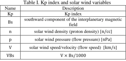
[image:5.595.57.276.491.677.2]The performances of regular and robust model with autoregressive terms are shown in Figure 1. The averaged correlation coefficients of regular and robust model are 0.748 and 0.759, and the averaged prediction efficiency of regular and robust model are 0.550 and 0.575, respectively. The overall performance of the robust model is slightly better than the regular model. In addition, for the last two test years, the improvements achieved by using robust structure are more significant than the first two years. The reason might be that the robust method is able to detect the significant model terms for each short period of data, which is extremely important because there exist many severe active times (Kp ) in the data. The improvement of prediction performance of theses active periods would largely improve the overall performance.
Figure 1. Performance comparison between the regular (blue) models and robust models (red) with autoregressive variables (left: correlation coefficient; right: prediction
efficiency)
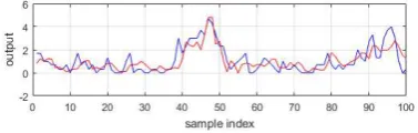
[image:5.595.304.496.560.685.2]prediction performance. However, there exists a common issue in these models with autoregressive variables, that is, there is a prediction lag. This lag is mostly caused by the inclusion of the autoregressive term Kp t in the model, which is highly correlated with Kp t , the model term selection algorithm usually selects it in the first step. The lag between the prediction and the corresponding measurement can be seen in Figure 2. The same phenomenon was also obviously observed in other linear and nonlinear models for example the NN model proposed in [2] has exactly the same issue.
Figure 2. Randomly selected 100 observed (red) and predicted (blue) Kp values of year 2012 (robust model with
autoregressive variables)
[image:6.595.101.287.197.257.2]C. Regular Model without Autoregressive Variables The regular model without autoregressive variables was identified based on the same train data as the regular model with autoregressive variables, but with only input lag variables. The OLS-ERR algorithm was employed for model term selection. The selected model terms of the model, along with the associated parameters, are shown in Table IV.
Table IV. Regular model without autoregressive variables
No Term ERR
(100%) Parameter 1 V t p t 79.0105 -1.7336e+02
2 VBs t Bs t 3.0698 -5.3816e+00
3 V t 0.4643 -2.8197e+01
4 VBs t Bs t 0.5121 3.3031e+00
5 Bs t Bs t 0.3814 1.2940e+01
6 p t VBs t 0.2651 1.7469e+02
7 V t V t 0.3667 4.5787e+01
8 p t p t 0.3884 -1.9329e+02
9 Bs t V t 0.2231 3.1549e+01 10 Bs t p t 0.0893 -1.6555e+02 11 V t V t 0.0660 -1.1536e+01
12 p t VBs t 0.0417 1.0354e+01
13 VBs t V t 0.0419 -2.8373e+00
The model in Table IV should read:
Kp t V t p t (18)
The performance of this model will be analyzed and discussed together with the robust model without autoregressive variables in the next section.
D. Robust Model without Autoregressive Variables The robust model without autoregressive variables was identified based on the same train data as the robust model with autoregressive variables, but with only input lag variables. In total, 13 model terms are selected by the proposed robust structure selection method. The parameters of these robust terms are estimated from the train data of year 2008.
Table V. Robust model without autoregressive variables
No Robust Term Parameter
1 V t p t 3.8385e+01
2 V t -2.4865e+01
3 V t 2.8368e+01
4 VBs t V t 1.7403e+00
5 n t VBs t 1.8330e+00
6 Bs t Bs t 1.4216e+01
7 Bs t Bs t 1.9646e+01
8 n t 9.6997e+00
9 Bs t 1.5046e+00
10 n t n t -1.2544e+01
11 Bs t Bs t -3.0055e+01
12 V t V t 2.2128e+01
13 Bs t V t 3.8385e+01
The model in Table V should read:
Kp t V t p t (19)
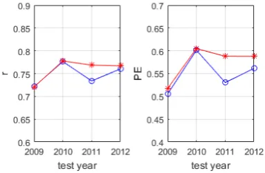
[image:6.595.86.304.405.593.2]The performances of regular and robust model without autoregressive terms are shown in Figure 3. The averaged correlation coefficients of regular and robust models are 0.669 and 0.689, and the averaged prediction efficiency of regular and robust model are 0.430 and 0.460, respectively. Clearly, the performance of robust and regular models without autoregressive variables are consistent with the models containing autoregressive variables: the overall performance of the robust model is better than the regular model, especially in the last two test years. Overall, the robust structure can help to improve the model performances, with and without autoregressive variables. Furthermore, the proposed robust model selection algorithm can be potentially applied to big data or long time period data modelling and prediction.
Figure 3. Performance comparison between the regular (blue) models and robust models (red) without autoregressive variables
(left: correlation coefficient; right: prediction efficiency)
[image:6.595.331.515.470.587.2]Yuanlin Gu; Hua-Liang Wei; Richard J. Boynton; Simon N. Walker; Michael A. Balikhin 6
Figure 4. Randomly Selected 100 observed (red) and predicted (blue) Kp values of year 2012 (robust model without
autoregressive variables)
VI. CONCLUSION
This study proposed a new robust model selection method for Kp index prediction. With the new selection algorithm, robust models with and without autoregressive variables were obtained for 3 hours ahead prediction of Kp index. The performance of the robust models was evaluated on the test data of 4 years. The correlation coefficient and prediction efficiency of the robust models are 0.748 and 0.759 (with autoregressive terms), 0.669 and 0.689 (without autoregressive terms), respectively. It turned out that the robust models outperform the regular models and more importantly, the robust model selection algorithm can successfully overcome a common issue encountered in most existing Kp prediction models, that is, there usually exist lags between the predictions and real measurements. The advantage of a robust model is that it can better capture the inherent dynamics of the whole dataset and can thus be well generalized to new data. With this advantage, the new robust selection method can potentially be applied to big data or long period data modelling problems.
ACKNOWLEDGMENT
The authors acknowledge that this work was supported in part by EU Horizon 2020 Research and Innovation Programme Action Framework under grant agreement 637302, the Engineering and Physical Sciences Research Council (EPSRC) under Grant EP/I011056/1 and Platform Grant EP/H00453X/1.
REFERENCES
[1] J. Bartels, The standardized index, Ks, and theplanetary, Kp, IATME Bull, 1949, 12b, 97.
[2] S. Wing, R. Johnson, J. Jen, C. I. Meng, D. G. Sibeck, K. Bechtold, J. Freeman, K. Costello, M. Balikhin, and K. Takahashi, Kp forecast models, J. Geophys. Res., 2005, 110(A4), A04203.
[3] V. O. Papitashvili, N. E. Papitashvili, and J. H. King, Solar Cycle Effects in planetary geomagnetic activity: Analysis of 36-year long OMNI dataset, Geophys. Res. Lett., 2000, 27, 2797-2800.
[4] H. A. Elliott, J. M. Jahn, and D. J. McComas, The Kp index and solar wind speed relationship: Insights for improving space weather forecasts, Space Weather, 2012, 11(6), 339-349. [5] P. T. Newell, T. Sotirelis, K. Liou, C. I. Meng, and F. J. Rich,
A nearlyuniversal solar wind-magnetosphere coupling function inferred from 10 magnetospheric state variables, J. Geophys. Res., 2007, 112(A1), A01206.
[6] K. A. Costello, Moving the Rice MSFM into a real-time forecast mode using solar wind driven forecast modules, Diss. Rice University, 1998.
[7] F. Boberg, P. Wintoft, H. Lundstedt, Real time Kp predictions from solar wind data using neural networks, Physics and Chemistry of the Earth, Part C: Solar, Terrestrial & Planetary Science, 2000, 25(4), 275-280.
[8] J. Takahashi, An automated oracle for verifying GUI objects, ACM SIGSOFT Software Engin. Notes, 2001, 26(4), 83-88.
[9] M. A. Balikhin, R. J. Boynton, S. N. Walker, J. E. Borovsky, S. A. Billings, H. L. Wei, Using the NARMAX approach to model the evolution of energetic electrons fluxes at geostationary orbit, Geophysical Research Letters, 2011, 38 (18).
[10] S. Chen, S. A. Billings and W. Luo, Orthogonal least squares methods and their application to non-linear system identification. International Journal of Control, 1989, 50(5), 1873-1896.
[11] M. A. Balikhin, O. M. Boaghe, S. A. Billings and H. St C. K. Alleyne, Terrestrial magnetosphere as a nonlinear resonator, Geophys. Res. Lett., 2001, 28, 1123-1126.
[12] J. R. Ayala Solares , H. L. Wei, R. J. Boynton, S. N. Walker, S. A. Billings,. Modeling and prediction of global magnetic disturbance in near Earth space: A case study for Kp index using NARX models, Space Weather, 2016, 14(10), 899-916. [13] S. Chen and S. A. Billings, Representations of non-linear
systems: the NARMAX model, International Journal of Control, 1989, 49(3), 1013-1032.
[14] A. M. Marshall, G. R. Bigg, S. M. van Leeuwen, J. K. Pinnegar, H. L. Wei, T. J. Webb, and J. L. Blanchard, Quantifying heterogeneous responses of fish community size structure using novel combined statistical techniques, Global Change Biology, 2015.
[15] G. R. Bigg, H. L. Wei, D. J. Wilton, Y. Zhao, S. A. Billings, E. Hanna, and V. Kadirkamanathan, A century of variation in the dependence of Greenland iceberg calving on ice sheet surface mass balance and regional climate change, Proc. R. Soc. A, 2014, 470(2166), 20130662.
[16] H. L. Wei, S. A. Billings, A. S. Sharma, S. Wing, R. J. Boynton, and S. N. Walker, Forecasting relativistic electron flux using dynamic multiple regression models, Annales Geophysicae, 2011, 29(2), 415-420.
[17] C. G. Billings, H. L. Wei, P. Thomas, S. J. Linnane, and B. D. M. Hope-Gill, The prediction of in-flight hypoxaemia using non-linear equations, Respiratory medicine, 2013, 107(6),841-847.
[18] H. L. Wei, S. A. Billings, and J. Liu, Term and variable selection for non-linear system identification, International Journal of Control, 2004, 77, 86-110.
[19] S. A. Billings, Nonlinear system identification: NARMAX methods in the time, frequency, and spatio-temporal domains, John Wiley & Sons, 2013.
[20] Y. Gu and H. L. Wei, Analysis of the relationship between lifestyle and life satisfaction using transparent and nonlinear parametric models, 22nd International IEEE Conference on Automation and Computing, 2016, 54-59.
[21] Y. Li, H. L. Wei, S. A. Billings, P. G. Sarrigiannis, Identification of nonlinear time-varying systems using an online sliding-window and common model structure selection (CMSS) approach with applications to EEG, International Journal of Systems Science, 2016, 47(11), 2671-2681. [22] G. H. Golub, M. Heath, and G. Wahba, Generalized
cross-validation as a method for choosing a good ridge parameter, Technometrics, 1979, 21(2), 215-223.
[23] S. A. Billings and H. L. Wei, An adaptive orthogonal search algorithm for model subset selection and non-linear system identification, International Journal of Control, 2008, 81(5), 7 [24] R. Bala, P. Reiff, Improvements in short term forecasting of
geomagnetic activity, Space Weather, 2012, 10(6).
[25] H. L. Wei and S. A. Billings, Improved model identification for non-linear systems using a random subsampling and multifold modelling (RSMM) approach, International Journal of Control, 2009, 82(1), 27-42.
[26] S. A. Billings, S. Chen, and M. J. Korenberg, Identification of MIMO non-linear systems suing a forward regression orthogonal estimator. International Journal of Control, 1989 49, 2157–2189.