Dirichlet Graph Densifiers

(1)

White Rose Research Online URL for this paper:

http://eprints.whiterose.ac.uk/105859/

Version: Accepted Version

Proceedings Paper:

Escolano, Francisco, Curado, Manuel, Lozano, Miguel Angel et al. (1 more author) (2016)

Dirichlet Graph Densifiers. In: Structural, Syntactic, and Statistical Pattern Recognition -

Joint IAPR International Workshop, S+SSPR 2016, Mérida, Mexico, November 29 -

December 2, 2016, Proceedings. Lecture Notes in Computer Science . Springer

International Publishing , pp. 185-195.

https://doi.org/10.1007/978-3-319-49055-7_17

[email protected] https://eprints.whiterose.ac.uk/

Reuse

Items deposited in White Rose Research Online are protected by copyright, with all rights reserved unless indicated otherwise. They may be downloaded and/or printed for private study, or other acts as permitted by national copyright laws. The publisher or other rights holders may allow further reproduction and re-use of the full text version. This is indicated by the licence information on the White Rose Research Online record for the item.

Takedown

If you consider content in White Rose Research Online to be in breach of UK law, please notify us by

(2)

Francisco Escolano, Manuel Curado, Miguel A. Lozano, and Edwin R. Hancook

Department of Computer Science and AI, University of Alicante, 03690, Alicante (Spain)

{sco,mcurado,malozano}@dccia.ua.es

Department of Computer Science, University of York, York, YO10 5DD, UK

[email protected]

Abstract. In this paper, we propose a graph densification method based on minimizing the combinatorial Dirichlet integral for the line graph. This method allows to estimate meaningful commute distances for mid-size graphs. It is fully bottom up and unsupervised, whereas anchor graphs, the most popular alternative, are top-down. Compared with an-chor graphs, our method is very competitive (it is only outperformed for some choices of the parameters, namely the number of anchors). In addition, although it is not a spectral technique our method is spectrally well conditioned (spectral gap tends to be minimized). Finally, it does not rely on any pre-computation of cluster representatives.

Keywords: Graph densification, Dirichlet problems, Random walkers

1 Introduction

1.1 Motivation

kNN graphs have been widely used in graph-based learning, since they tend to capture the structure of the manifold where the data lie. However, it has been re-cently noted [1] that for a standard machine learning setting (n→ ∞,k≈logn

and larged, wherenis the number of samples anddis their dimension) we have that kNN graphs result in a sparse, globally uninformative representation. In particular, a kNN-based estimation of the geodesics (for instance through the shortest paths as done in ISOMAP) diverges significantly unless we assign proper weights to the edges of thekNN. Finding such weights is a very difficult task asd

(3)

other words, for a sufficient number of anchors it is then possible to find links between distant regions of the space. As a result, the problem of finding suitable weights for the graph is solved through kernel-based regression.

Data-to-anchorkNN graphs are computed fromm≪nrepresentatives (an-chors) typically obtained through K-means clustering, inO(dmnT+dmn), where

O(dmnT) is due to the T iterations of the K-means process. Since m ≪ m, the process of constructing the m ×m affinity matrix W = ZΛZT_{, where}

Λ= diag(ZT_{1) and}_Z_{is the data-to-anchor mapping matrix, is linear in}_n_{. As a} byproduct of this construction, we have that the mainr eigenvalue-eigenvector pairs associated withM =Λ−1/2ZTZΛ−1/2, which has also dimensionm×m, lead a compact solution for the spectral hashing problem [14] (see [9] for details). These eigenvectors-eigenvalues may also provide a meaningful estimation of the commute distances between the samples through the spectral expression of this distance [11].

Once considered the benefits of anchor graphs, their use is quite empirical since their foundations are poorly understood. For instance, the choice of the

m representatives is quite open and heuristic. The K-means selection process outperforms the uniform selection because it approximates better the underly-ing distribution. More clever oracles for estimatunderly-ing not only the positions of the representatives but also their number would lead to interesting improvements. However, the developments of these oracles must be compatible with the un-derlying principle defining an anchor graph, namelydensification. Densification refers to the process of increasing the number edges (or the weights) of an input graph so that the result preserves and even enforces the structural properties of the input graph. This is exactly what it anchors provide: given a sparse graph associated to a standard machine learning setting, they produce a more com-pact graph which is locally dense (specially around the anchors) and minimizes inter-class paths.

Graph densification is a principled study of how to significantly increase the number of edges of an input graph Gso that the output, H, approximatesG

with respect to a given test function, for instance whether there exists a given cut. Existing approaches [4] pose the problem in terms of semidefinite program-ming SDP where a global function is optimized. These approaches have two main problems: a) the function to optimize is quite simple and does not impose the minimization of inter-class edges while maximizing intra-class edges, and b) since the number of unknowns is O(n2_{), i.e. all the possible edges, and SDP solvers}

(4)

1.2 Contributions

In this paper, we propose a bottom-up graph densification approach which com-mences by grouping edges through return random walks (Section 2). Return random walks (RRW) are designed to enforce intra-class edges while penalizing inter-class weights. Since our strategy is completely unsupervised, return random walks operate under the hypothesis that inter-class edges are rare events. Given input sparse graph G(typically resulting from a thresholded similarity matrix

W), RRWs produce a probabilistic similarity matrixWe. Then, high probability edges are assumed to drive the grouping process. To this end, we exploit the

random walker[3] but in the edges space (Section 3). The random walker

min-imizes the Dirichlet integral, in this case that associated with the line graph of

We:LineWe. Given a set of known edges (assumed to be the ones with maximal

probability inWe) we predict the remainder edges. The result is a locally-dense graphH that is suitable for computing commute distances. In our experiments (Section 4), we will compare our Dirichlet densifier with anchor graph as well as with existing non-spectral alternatives relying exclusivelly onkNN graphs.

vi vj

vk

vl vk

vl TRANSITION NODES

CLUSTER #1

CLUSTER #2

ORIGIN DESTINATION

vi vj

vk

vl

vj

vk

vl

TRANSITION NODES

ORIGIN DESTINATION

GO

RETURN

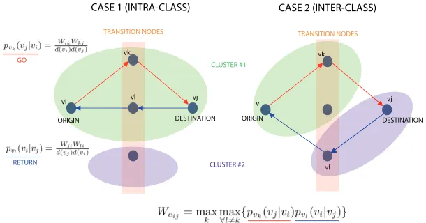
CASE 1 (INTRA-CLASS) CASE 2 (INTER-CLASS)

[image:4.595.155.460.338.498.2]

HYPOTHESIS: Probability of CASE 1 is higher than the probability of CASE 2

Fig. 1.Return random walks for reducing inter-class noise.

2 Return Random Walks

Given a set of points χ = {x₁, ...,x_n} ⊂ Rd, we map the x_i to the vertices

V of an undirected weighted graph G(V, E, W). We have that V is the set of nodes where each vi represents a data pointxi , E⊆V ×V is the set of edges linking adjacent nodes. An edgee= (i, j) withi, j∈V, exists if Wij>0 where

Wij =e−σ||xi−xj||

2

(5)

Design of W e. GivenW we produce a reweighted similarity matrixWeby following this rationale: a) we explore the two-step random walks reaching a node

vjfromvithrough any transition nodevk, b)on returnfromvjtoviwe maximize the probability of returning through a different transition nodevl6=vk. For the first step (going fromvi tovj throughvk) we havepvk(vj|vi) =

WikWkj

d(vi)d(vj) as well

as astandard returnpvl(vi|vj) =

WjlWli

d(vj)d(vi). Standard return works pretty well if

vi andvj belong to the same cluster (see Fig. 1-left). However,vl(the transition node for returning) can be constrained so that vl 6=vk. In this way, travelling out of a class is penalized since the walker must choose a different path, which in turn is hard to find on average. Therefore, we obtainWeij fromWij as follows:

Weij = max

k max∀l6=k{pvk(vj|vi)pvl(vi|vj)}, (1)

i.e. for each possible transition node vk we compute the probability of go and return (product of independent probabilities) through a different node vl. We retain the maximum product of probabilities for each vl referred to a given k and finally we retain the supremum of these maxima. As a result, when inter-class travels are frequent for a given e = (i, j) (Fig. 1-right) its weight Weij

is significantly reduced. Our working hypothesis is that the number of edges subject to this condition is small on average, since the number of inter-class edges tends to be small compared with the total number of edges. However, in realistic situations where patterns can be confused due either to their intrinsic similarity or to the use of an unproper similarity measure, this assumption leads to a significant decrease of many weights ofW.

3 The Dirichlet Graph Densifier

3.1 The Line Graph

The graph densification problem can be posed as follows: given a graph G = (V, E, W) infer another graphH= (V, E′, W′) so that|E′| ≥ |E|in such a way that the bulk of the increment in the number of edges is constrained to intra-class edges (i.e. the number of inter-class edges is minimized). Therefore, the unknowns of the problem are the new edges to infer, not the vertices. In principle we have a O(n2) unknowns, wheren =|V|, but working with all of them is infeasible. This motivates the selection of a small fraction of them (those with the highest values ofWeij) according to a given thesholdγe. The counterintuitive fact that

the smaller the fraction the better the accuracy is explained below and showed later in the experimental section. Concerning efficiency, the first impact of this choice is that only |E′′_| _{edges, with} _|_E′′_{| ≪ |}_E_| _{are considered for building a}

graph of edges, i.e. a line graph LineWe. Let A thep×n edge-node incidence

matrix defined as follows:

Aeijvk= 





+1 ifi=k,

−1 ifj=k,

0 otherwise,

(6)

Then, the C = AAT −2Ip is the adjacency matrix of an unweighted line graph, where: Ip is thep×pidentity matrix, the nodes ea are given by all the possible pairs of r = |E′′| edges with a common vertex according to A. The edges of C implement second-order interactions between nodes in the original graph from which A comes from. However, C is still unattributed (although conditioned byWe). A proper weighting of for this graph is to use standard ”go and return” random walks, i.e.

LineWe(ea, eb) =

r

X

k=1

pek(eb|ea)pek(ea|eb), (3)

i.e. return walks are not applied because they become too restrictive. Then, there is an edge in the line graph for every pair (ea, eb) with LineWe(ea, eb)>0. We

denote the set os edges of the line graph byELine

3.2 The Dirichlet Functional for the Line Graph

Given the line graph LineWe with r nodes (now edges) many of them will be

highly informative according to We and the application of Eq. 3. We retain a fraction of them (again, those with the largest values of We) according to a second thresholdµe. This threshold must be set as smaller as possible since it defines the difference between the ”known” and the ”unknown”. More precisely,

We acts as a function We : |E′′| → R so that the larger its value the more trustable is a given edge as an stable or known edge in the original graph G. Unknown edges are assumed to have small values ofWeand this is why they are not selected, since the purpose of our method is to infer them.

This is a classical inference problem, now in the space of edges and completely unsupervised, which has been posed in terms of minimizing the disagreements between the weights of existing (assumedto be ”known”) edges and those of the ”unknown” or inferred ones. In this regard, since unknown edges are typically neighbors of known ones, the minimization of this disagreement is naturally expressed in terms of finding an harmonic function. Harmonic functions u(x) satisfy∇2_u_{= 0 which in our discrete setting leads to the following property}

u(ea) = 1

d(ea)

X

(ea,eb)∈ELine

LineWe(ea, eb)u(eb), (4)

The harmonic function u(.) is not unconstrained, since it is known for some values of the domain (the so called boundary). In our case, we setu(ea) =Wea

forea∈EB, referred to asborder nodessince they are associated with assumed known edges. The harmonic function is unknown foreb ∈EI =E′′ ∼EB (the

inner nodes). Then, finding an harmonic function given boundary values is called

theDirichlet problem and it is typically formulated in terms of minimizing the

following integral

D[u] = 1 2

Z

Ω

(7)

whose discrete version relies on the graph Laplacian [3] (in this case on the Laplacian of the line graph):

DLine[u] = 1 2(Au)

T_R₍_Au_{) =} 1 2u

T_L Lineu

=1 2

X

(ea,eb)∈ELine

LineWe(ea, eb)(u(ea)−u(eb))

2_, ₍₆₎

d(ea) =Peb6=eaLineWe(ea, eb) is the diagonal degree matrix. Then,LLine is the

Laplacian of the line graph.

Given the LaplacianLLineand the Dirichlet combinatorial integralDLinewe have that the nodes in the line graph are partitioned in two classes: ”border” and ”inner”, i.e.E” =EB∪EI. This partition leads to a reordering of the harmonic function u= [uBuI] as well as the Dirichlet integral:

D

uI=1₂uTB uTI

LB K

KT LI

uB

uI

(7)

whereD

uI= 1₂(uTBLBuB+ 2uTIKTUB+uTILIuI) and differentiating w.r.t.uI leads to solve a linear system which relatesuI withuB:

LIuI =−KTuB. (8)

Then, lets∈[0,1] be a label indicating to what extend a given node of the line graph (an edge in the original graph) is relevant. We define a potential function

Q : EB → [0,1] so that for a known node ea ∈ EB we assign a label s, i.e.

Q(ea) =s. This leads to declaring the following vector for each label:

ms_a =

( _W

ea

max_eb∈_E”{W_eb} ifQ(ea) =s,

0 ifQ(ea)6=s

. (9)

Finally, the linear system is posed in terms of how the known labels do predict the unknown ones, placed in the vectoru, as follows:

LIus=−KTms. (10)

If we consider simultaneously all labels instead of a single one, we have

LIU=−KTM ⇒U = (−KTM)L−I1, (11)

whereU is a vector of|EI|rows (one per unknown/inner edge,known solved) and

(8)

known, and the remainder are denoted by eb) and the edges in the original graph G = (V, E, W), then we have that ek corresponds to edge (i, j) ∈ E. However, since its weight has potentially changed after solving the linear system, we adopt the following densification criterion (labeling) for creating the graph

H = (V, E, W′_):

Hij =







maxek∈UUkifek ∈EI

Mij ifek ∈EB,

0 otherwise

(12)

In this way, the edgesE′ _{of the dense graphs are given by}_H

ij >0.

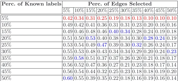
Perc. of Known labels Perc. of Edges Selected

5% 10% 15% 20% 25% 30% 35% 40% 45% 50%

5% 0.42 0.34 0.31 0.25 0.19 0.18 0.13 0.10 0.10 0.10

10% 0.49 0.42 0.41 0.36 0.31 0.31 0.23 0.20 0.16 0.16 15% 0.49 0.46 0.48 0.460.40 0.340.28 0.24 0.19 0.18 20% 0.51 0.500.53 0.40 0.38 0.34 0.300.28 0.240.19 25% 0.53 0.54 0.490.470.39 0.300.32 0.26 0.24 0.17 30% 0.55 0.53 0.48 0.43 0.34 0.34 0.29 0.20 0.240.23

[image:8.595.156.459.252.390.2]

35% 0.590.580.51 0.37 0.37 0.26 0.20 0.21 0.18 0.17 40% 0.56 0.52 0.47 0.36 0.27 0.21 0.23 0.18 0.17 0.14 45% 0.56 0.54 0.44 0.32 0.25 0.23 0.18 0.18 0.19 0.20 50% 0.600.55 0.39 0.35 0.22 0.18 0.16 0.19 0.16 0.14 Table 1.Dirichlet densifier: Accuracy for the reduced NIST database

4 Experiments and Conclusions

(9)

20 40 60 80 100 120 140 160 180 200 20 40 60 80 100 120 140 160 180 200

DENSIFICATION WITH 5% OF EDGES SELECTED AND 5% KNOWN LABELS

(a)

20 40 60 80 100 120 140 160 180 200 20 40 60 80 100 120 140 160 180 200

APPROXIMATE COMMUTE TIMES OF DENSIFICATION WITH 5% OF EDGES SELECTED AND 5% KNOWN LABELS

(b)

20 40 60 80 100 120 140 160 180 200 20 40 60 80 100 120 140 160 180 200

(c)

20 40 60 80 100 120 140 160 180 200 20 40 60 80 100 120 140 160 180 200

(d)

20 40 60 80 100 120 140 160 180 200 20 40 60 80 100 120 140 160 180 200

(e)

20 40 60 80 100 120 140 160 180 200 20 40 60 80 100 120 140 160 180 200

[image:9.595.164.452.171.548.2]

(f)

Fig. 2.Densification result and its associate Approximate commute times (ACT) ma-trix for different fractions of known labels |E_B_| _{and leading edges} _|E_{”|: (a)}

Densifi-cation with |E_B_|_{= 5%,} _|E_”| _{= 5%, (b) corresponding ACT , (c) Densification with}

|E_B_|_{= 50%,}_|E_”|_{= 5%, (d) corresponding ACT , (e) Densification with}_|E_B_|_{= 50%,}

(10)

Number of anchors

25 50 75 100 125 150

Accuracy (%)

0.1 0.2 0.3 0.4 0.5 0.6

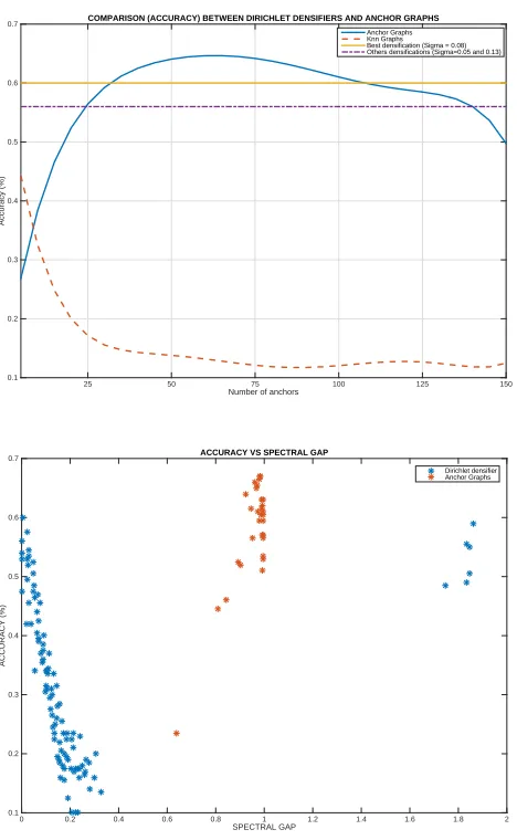
0.7 COMPARISON (ACCURACY) BETWEEN DIRICHLET DENSIFIERS AND ANCHOR GRAPHS

Anchor Graphs Knn Graphs Best densification (Sigma = 0.08) Others densifications (Sigma=0.05 and 0.13)

SPECTRAL GAP

0 0.2 0.4 0.6 0.8 1 1.2 1.4 1.6 1.8 2

ACCURACY (%)

0.1 0.2 0.3 0.4 0.5 0.6

0.7 ACCURACY VS SPECTRAL GAP

[image:10.595.193.427.176.556.2]

Dirichlet densifier Anchor Graphs

Fig. 3.Top: Accuracy of Anchors Graphs,k_{NN Graphs and Dirichlet densifiers.}

(11)

approximation of the commute distance (d) w.r.t. retaining 50% of the edges to build the line graph. The commute distances after retaining 50% are meaningless (f) despite the obtained graph is denser. In all cases, the error assumed when approximating the commute times matrix is ǫ= 0.25.

In a second experiment, we compare the commute distances obtained with the optimal Dirichlet densifier (fraction of retained leading edges |E”| = 5%| and fraction known labels|EB|= 50%) with different settings for the anchor graphs. Concerning anchor graphs, in all cases we setσ= 0.08 for constructing the Gaus-sian graphs from the raw input data. In our Dirichlet approach we use the same setting. This provides the best result in the rangeσ∈[0.05,0.13]. In Fig. 3-Left we show how the accuracy evolves while increasing the number of (anchors)m: from 5 to 150. The performance of anchor graphs increases withmbut degrades after reaching the peak atm= 70 (accuracy 0.67). This peak is due to the fact that anchor graphs tend to reduce the amount of inter-class noise. However, this often leads to poor densification. On the other hand, Dirichlet densifiers they are completely unsupervised and do not rely on anchor computation. Their perfor-mance is constant w.r.t.mand the best accuracy is 0.60. We outperform anchor graphs form <35 andm >105 and in the rangem∈[35,105] our best accuracy is very close to the anchor graph’s performance. Regarding existing approaches that compute commute distances from standard weightedkNN graphs [6][5] we outperform them for any choice ofm, since their performace degrades very fast withmdue to the intrinsic inter-class noise arising in realistic databases.

Finally, we reconcile our results, and those of the anchor graphs with the von Luxburg and Radl’s fundamental bounds. In principle, commute distances cannot be properly estimated from large graphs [13]. However, in this paper we show that both anchor graphs and Dirichlet densifiers provide meaningful commute times. It is well known that this can be done insofar the spectral gap is close to zero or the minimal degree is close to the unit. Dirichlet densifiers provide spectral gaps close to zero (see Fig. 3-Right) for low fractions of leading edges, but the accuracy degrades linearly when the spectral gap increases. This means that the spectral gap is negatively correlated with increasing fractions of inter-class noise. This noise arises when the densification level increases since Dirichlet densifiers are not still able of confining densification to intra-class links. Concerning anchor graphs, their spectral gap is close to the unit since the de-gree also the unit (double-stochastic matrices) and they outperform Dirichlet densifiers to some extent at the cost of computing anchors and finding the best number of them.

To conclude, we have contributed with a novel method for transforming input graphs into denser versions which are more suitable for estimating meaningful commute distances in large graphs.

References

(12)

2. Cai, D., Chen, X.: Large scale spectral clustering via landmark-based sparse rep-resentation. IEEE Trans. Cybernetics45(8) (2015) 1669–1680

3. Grady, L.: Random walks for image segmentation. IEEE Trans. Pattern Anal. Mach. Intell.28(11) (2006) 1768–1783

4. Hardt, M., Srivastava, N., Tulsiani, M.: Graph densification. In: Innovations in Theoretical Computer Science 2012, Cambridge, MA, USA, January 8-10, 2012. (2012) 380–392

5. Khoa, N.L.D., Chawla, S.: Large scale spectral clustering using approximate com-mute time embedding. CoRRabs/1111.4541(2011)

6. Khoa, N.L.D., Chawla, S.: Large Scale Spectral Clustering Using Resistance Dis-tance and Spielman-Teng Solvers. In: Discovery Science: 15th International Con-ference, DS 2012, Lyon, France, October 29-31, 2012. Proceedings. Springer Berlin Heidelberg, Berlin, Heidelberg (2012) 7–21

7. Liu, W., He, J., Chang, S.: Large graph construction for scalable semi-supervised learning. In: Proceedings of the 27th International Conference on Machine Learning (ICML-10), June 21-24, 2010, Haifa, Israel. (2010) 679–686

8. Liu, W., Wang, J., Chang, S.: Robust and scalable graph-based semisupervised learning. Proceedings of the IEEE100(9) (2012) 2624–2638

9. Liu, W., Wang, J., Kumar, S., Chang, S.: Hashing with graphs. In: Proceedings of the 28th International Conference on Machine Learning, ICML 2011, Bellevue, Washington, USA, June 28 - July 2, 2011. (2011) 1–8

10. q. Luo, Z., k. Ma, W., c. So, A.M., Ye, Y., Zhang, S.: Semidefinite relaxation of quadratic optimization problems. IEEE Signal Processing Magazine27(3) (2010) 20–34

11. Qiu, H., Hancock, E.R.: Clustering and embedding using commute times. IEEE Trans. Pattern Anal. Mach. Intell.29(11) (2007) 1873–1890

12. Spielman, D.A., Srivastava, N.: Graph sparsification by effective resistances. SIAM J. Comput.40(6) (2011) 1913–1926

13. von Luxburg, U., Radl, A., Hein, M.: Hitting and commute times in large random neighborhood graphs. Journal of Machine Learning Research15(1) (2014) 1751– 1798