Mixture of Circular and Noncircular Sources
.
White Rose Research Online URL for this paper:
http://eprints.whiterose.ac.uk/99229/
Version: Accepted Version
Article:
Chen, H., Hou, C., Liu, W. orcid.org/0000-0003-2968-2888 et al. (2 more authors) (2016)
Efficient Two-Dimensional Direction-of-Arrival Estimation for a Mixture of Circular and
Noncircular Sources. IEEE Sensors Journal, 16 (8). pp. 2527-2536. ISSN 1530-437X
https://doi.org/10.1109/JSEN.2016.2517128
© 2016 IEEE. Personal use of this material is permitted. Permission from IEEE must be
obtained for all other users, including reprinting/ republishing this material for advertising or
promotional purposes, creating new collective works for resale or redistribution to servers
or lists, or reuse of any copyrighted components of this work in other works.
[email protected] https://eprints.whiterose.ac.uk/ Reuse
Unless indicated otherwise, fulltext items are protected by copyright with all rights reserved. The copyright exception in section 29 of the Copyright, Designs and Patents Act 1988 allows the making of a single copy solely for the purpose of non-commercial research or private study within the limits of fair dealing. The publisher or other rights-holder may allow further reproduction and re-use of this version - refer to the White Rose Research Online record for this item. Where records identify the publisher as the copyright holder, users can verify any specific terms of use on the publisher’s website.
Takedown
If you consider content in White Rose Research Online to be in breach of UK law, please notify us by
Efficient Two-Dimensional Direction of Arrival
Estimation for a Mixture of Circular and
Noncircular Sources
Hua Chen, Chunping Hou, Wei Liu, Senior Member, IEEE, Wei-Ping Zhu, Senior
Member, IEEE and M.N.S. Swamy, Fellow, IEEE
Abstract—In this paper, the two-dimensional (2-D) direction-of-arrival (DOA) estimation problem for a mixture of circular and non-circular sources is considered. In particular, we focus on a 2-D array structure consisting of two parallel uniform linear arrays (ULAs) and build a general array model with mixed circular and non-circular sources. The received array data and its conjugate counterparts are combined together to form a new data vector, based on which a series of 2-D DOA estimators are derived. Compared to existing methods, the proposed one has three main advantages. Firstly, it can give a more accurate estimation in situations where the number of sources is within the traditional limit of high resolution methods; secondly, it can still work effectively when the number of mixed signals is larger than that of the array elements; thirdly, the paired 2-D DOAs of the proposed method can be obtained automatically without the complicated 2-D spectrum peak search and therefore has a much lower computational complexity.
Index Terms—Two-dimensional (2-D), Direction of arrival (DOA), non-circular signal, rank-reduction, planar arrays
I. INTRODUCTION
T
HE estimation of two-dimensional (2-D) direction ofar-rival (DOA) is an important area of array signal process-ing and has received much attention in past years [1, 2]. Many effective methods and algorithms have been proposed based on different array structures, such as two-parallel uniform linear arrays (ULAs) [3–7], L-shaped ULAs [8–13], and uniform rectangular arrays (URAs) [14–16].
In most traditional DOA estimation algorithms, only the traditional covariance matrix is considered which characterizes the circular Gaussian distribution and in recent years, the DOA estimation problem for non-circular signals has attracted more and more attention, first for one-dimensional (1-D) or linear arrays [17–25], and then extended to the 2-D case [26–28]. By exploiting this additional noncircularity information, an improved performance can be achieved for both 1-D and 2-D DOA estimation. In particular, in [26], Liu. et al proposed an ERARE method for noncircular sources based on two-parallel ULAs, with improved estimation accuracy compared
This work is supported by the National 863 Programs under Grant (No. 2015AA01A706) and China Scholarship Council (CSC).
Hua Chen, Chunping Hou are with the School of Electronic Information En-gineering, Tianjin University, China, 300072. (e-mail: [email protected].) Wei Liu is with the Department of Electronic and Electrical Engineering, University of Sheffield, Sheffield S1 3JD, UK. (e-mail: [email protected]). Wei-Ping Zhu and M.N.S. Swamy are with the Department of Electrical and Computer Engineering, Concordia University, Montreal, QC H3G 1M8, Canada. (e-mail: [email protected]; [email protected]).
to [4]; based on [13], the estimation accuracy was also improved with the conjugate information of the observed data for L-shaped ULAs in [27]. By employing non-circular signal constellations, Roemer and Haardt proposed a DOA estimation algorithm for a regular-hexagonal shaped ESPAR array, with a detailed analysis of the Cramer-Rao bound (CRB) [28].
A more general problem is that the impinging signals to the array are a mixture of circular and non-circular ones, such as a mixture of quadrature phase shift keying (QPSK) signals (circular) and binary phase shift keying (BPSK) signals (non-circular). This problem has been studied for DOA estimation of 1-D arrays and several approaches have been proposed [29– 31]. In [29], a new data vector was formed by combining the original data and its conjugate version to construct two estimators for direction finding of circular and non-circular signals, respectively. However, it can not deal with the problem when the DOAs of the circular and non-circular signals are coincident, and a small angle separation between them will lead to severe performance degradation. An improved algo-rithm was then proposed in [30], which estimates the DOAs of circular and non-circular signals separately by exploiting the difference between the circularity properties of the signals. Nevertheless, when the number of data samples is small, its DOA estimation performance will degrade. In [31], the problem was solved using a sparse representation algorithm, which employs overcomplete dictionaries subject to sparsity constraints to jointly represent the covariance and elliptic covariance matrices of the array output. However, to our best knowledge, the 2-D DOA estimation problem for mixed circular and non-circular impinging signals has not yet been addressed in literature.
2 1
Z
M
dx Y
thekth signal
dy
k
θ
k
β
[image:3.612.313.562.346.493.2]X
Fig. 1. Geometry of the array model.
of our proposed method. Throughout the paper, (·)∗
, (·)T, (·)−1 and(·)H represent
conjugation, transpose, inverse and conjugate transpose, re-spectively.E(·)is the expectation operation;diag(·)stands for the diagonalization operation; Ipdenotes thep×pdimensional
identity matrix; det[·] is the determinant of a matrix.
II. PROBLEMFORMULATION
As shown in Fig.1, suppose that there areK=Kn+Kc
un-correlated far-field sources impinging upon the array withKn
noncircular sources sn,k(t) and Kc circular sources sc,k(t),
from directions (θk, βk), k = 1,2, . . . , K. The array consists
of two parallel ULAs with each one havingM elements. The
distance between the two ULAs isλ/2, denoted asdy, and the
inter-element spacingdxfor each ULA is alsoλ/2, whereλis
the wavelength of the incident waves. The additive noises of the two ULAs are circular Gaussian with zero mean and
vari-ance σ2, which are uncorrelated with the impinging signals.
The output data vectors x(t) = [x1(t), x2(t), . . . , xM(t)] and
y(t) = [y1(t), y2(t), . . . , yM(t)] of the two ULAs at sample t
can be modeled as
x(t) =A˜s(t) +nx(t) (1)
y(t) =AB˜s(t) +ny(t) (2)
where A is the steering matrix with each column denoted by a(θk), given by a(θk) = [a0(θk), . . . , aM−1(θk)]T with ai(θk) = e−j
2π
λdx(i) cosθk, B(β) is termed as the steering
element matrix given by B = diag[v(β1), v(β2), . . . , v(βK)], with v(βk) = ej
2π
λdycosβk, n
x(t) = [nx,1(t), . . . , nx,M(t)]T
and ny(t) = [ny,1(t), . . . , ny,M(t)]T represent the circu-lar Gaussian noise vectors of the two arrays, respectively,
and ˜s(t) = [sn,1(t), ..., sn,Kn(t), sc,1(t), ..., sc,Kc(t)]
T is the
mixed source signal vector which has the following form
˜s(t) = ˙Bs(t) (3)
In (3),B is given by˙
˙
B=diag
bn,1, ..., bn,Kn,1,· · ·,1 | {z }
Kc
=
˙
B1 0
0 B˙2
(4)
where B˙1 = diag [bn,1, ..., bn,Kn], B˙2 = IKc, and s(t) is
defined as
s(t) = [¯sn,1(t), ...,¯sn,Kn(t), sc,1(t), ..., sc,Kc(t)]
T. (5)
We assumesn,k(t)is a strictly noncircular (rectilinear)
sig-nal [32, 33]. Then it can be expressed assn,k(t) =bn,ks¯n,k(t),
wheres¯n,k(t)is a real signal, andbn,k=ejϕk(k= 1, ..., Kn)
is an arbitrary phase shift for the signal.
III. THEPROPOSEDMETHOD
In this section, the 2-D DOA estimation algorithm for a general mixture of circular and non-circular signals impinging on the two parallel ULAs is derived in detail, based on the observed data coupled with its conjugate counterparts.
A. General array model
By concatenating the observed data vectors x(t) and y(t), we define a new data vector z(t)as follows
z(t)=
x(t) y(t)
=
A(θ) A(θ)B(β)
˙ Bs(t) +
nx(t)
ny(t)
=C(θ, β) ˙Bs(t) +n(t).
(6)
For simplified notation, the pair of angles (θ, β) together
with t are omitted in the following when not causing any
confusion.
In (6), C(θ, β)is named as the extended steering vector with
each column denoted as c(θ, β) , which can be expressed as
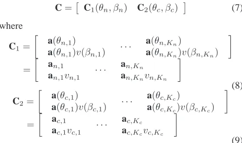
C= C1(θn, βn) C2(θc, βc)
(7)
where
C1=
a(θn,1)
a(θn,1)v(βn,1)
· · · a(θn,Kn)
a(θn,Kn)v(βn,Kn)
=
an,1
an,1vn,1 · · ·
an,Kn
an,Knvn,Kn
(8)
C2=
a(θc,1)
a(θc,1)v(βc,1) · · ·
a(θc,Kc)
a(θc,Kc)v(βc,Kc)
=
ac,1
ac,1vc,1 · · ·
ac,Kc
ac,Kcvc,Kc
(9)
are2M×Kn and2M×Kc matrices, respectively.
Then, another new data vector ˘z is defined by combining
the vector z and its conjugate counterpart z∗ as follows
˘z=
z z∗
=
CBs˙ C∗B˙∗s∗
+
n n∗
= ˘C˘s+ ˘n (10)
whereC is a˘ 4M ×(Kn+ 2Kc)matrix, i.e.,
˘
C= [˘cn,1, ...,˘cn,Kn,C˘c,1, ...,C˘c,Kc] (11)
with
˘cn,k =
bn,k
an,k
an,kvn,k
b∗n,k
a∗n,k a∗n,kv∗
n,k
(12)
being a4M×1 vector (k= 1,2, . . . , Kn), and
˘
Cc,k=
ac,k
ac,kvc,k
0M×1 0M×1
0M×1 0M×1 a∗c,k a∗
c,kv ∗ c,k
being a 4M ×2matrix (k= 1,2, . . . , Kc),
˘s= [sn,1, ..., sn,Kn, sc,1, s
∗
c,1, ..., sc,Kc, s
∗ c,Kc]
T (14)
is a(Kn+ 2Kc)×1vector, and
˘ n= n n∗ (15)
is a4M×1 vector.
Based on the above general array model, the proposed method is derived in the following section.
B. Main method
The covariance matrix of˘z is given by
˘
R=E[˘z˘zH] = ˘CR˘sC˘
H
+σ2I4M (16)
whereR˘s=E[˘s˘sH] is the covariance matrix of˘s.
Remark 1: In practice, only a finite number of observed data is available. Thus, R is estimated by˘
¯ ˘
R≈ 1
L L
X
l=1
˘z(l)˘zH(l), (17)
whereLdenotes the number of snapshots. With less observed
data, there will be a larger error in the estimated covariance matrix, which will lead to a degradation in performance.
Since the signals are not correlated with each other,R˘sis a
full rank matrix. Then the eigen-value decomposition (EVD) ofR is˘
˘
R=EsΣsEH
s +EnΣnEHn (18)
where the4M×(Kn+ 2Kc)matrixEsand the4M×(4M−
Kn −2Kc) matrix En are the signal subspace and noise
subspace, respectively. The(Kn+ 2Kc)×(Kn+ 2Kc)matrix
Σs= diag(λ1,λ2· · ·,λK)and the(4M−Kn−2Kc)×(4M−
Kn−2Kc)matrixΣn = diag(λK+1,λK+2· · ·,λ4M)are the
corresponding diagonal matrices, where λ1 ≥ λ2 ≥ · · · ≥
λK > λK+1=· · ·=λ4M =σ2 are the eigenvalues of R.˘
Considering that both C and˘ Es span the signal subspace,
which are orthogonal to the noise subspace spanned by the
matrix En, we derive the following estimators to obtain the
2-D DOAs of noncircular and circular signals using the rank-reduction method.
1) 2-D DOA estimation for noncircular sources: Based on
the orthogonality betweenEnand˘cn,k, the following equation
holds for any direction from(θn,k, βn,k)
EHn˘cn,k=0 (19)
In order to avoid the 2-D spectrum peak search related to (θn,k, βn,k) in a grid area, together with (13), (19) can be
rewritten as
0
=EHn˘cn,k
=EHn
bn,k an,k
an,kvn,k
b∗ n,k a∗ n,k a∗ n,kv ∗ n,k
=EHn
bn,k
an,k 0M×1
0M×1 an,k
1
vn,k
b∗n,k
a∗n,k 0M×1 0M×1 a∗n,k
1 v∗ n,k
=EHn
an,k an,k a∗ n,k a∗ n,k bn,k bn,kvn,k
b∗ n,k b∗ n,kv ∗ n,k
=EHn
an,k an,k
a∗n,k a∗n,k
1 0
vn,k 0
0 1
0 v∗
n,k bn,k b∗ n,k (20)
Defining a4M×4 matrixΩ(θ)which is only related toθ
Ω(θ) =
a(θ) a(θ)
a∗( θ)
a∗( θ) (21) and
pn(θ) =ΩH(θ)EnEHnΩ(θ) (22)
we obtain the following estimator over θ corresponding to
noncircular signals as
fn(θ) = [det(pn(θ))]
−1= [det(ΩH(θ)E
nEHnΩ(θ))] −1 (23)
If searched over the confined region with θ ∈ [0, π], the
DOAsθn,k of noncircular sources can be obtained from peaks
infn.
We then substitute the estimated θ of noncircular sources
into (20) and have the following estimator overβ
correspond-ing to noncircular signals
fn′(β) = [det(p′n(β)))]−1 (24)
where
p′n(β) =ΘH(β)ΩH(θ)EnEHnΩ(θ)Θ(β) (25)
and
Θ(β)=
1 0
v(β) 0
0 1
0 v∗
(β)
(26)
2) 2-D DOA estimation for circular sources: The
orthogo-nality betweenEn andC˘c,k still holds, i.e.
EHnC˘c,k =EHn
ac,k
ac,kvc,k
0M×1 0M×1
0M×1 0M×1 a∗c,k a∗ c,kv ∗ c,k
From (27), we have
EHn
ac,k
ac,kvc,k
0M×1 0M×1
=0 (28)
and
EHn
0M×1 0M×1 a∗c,k a∗c,kv∗
c,k
=0 (29)
Partitioning the matrix En into En = [ETn1,ETn2]T, where
En1 and En2 are two submatrices of the same size 2M ×
(4M−Kn−2Kc), (28) and (29) can be changed to
0
=
ac,k
ac,kvc,k
H
En1EHn1
ac,k
ac,kvc,k
= 1 vc,k H ac,k ac,k H
En1EHn1
ac,k ac,k 1 vc,k (30) and 0= ac,k
ac,kvc,k
∗H
(En2EHn2)
ac,k
ac,kvc,k
∗
⇒0=
ac,k
ac,kvc,k
H
E∗n2(E∗n2)H
ac,k
ac,kvc,k
⇒ 0
=
ac,k
ac,kvc,k
H
(En2EHn2)∗
ac,k
ac,kvc,k
= 1 vc,k H ac,k ac,k H
(En2EHn2)
∗ × ac,k ac,k 1 vc,k (31) As shown in Appendix, (30) and (31) are equivalent to each other.
Here, based on (30), the estimator overθ corresponding to
circular signals is as follows.
Since
1
vc,k
6
=0 (32)
we have
fc(θ) = [det(pc(θ))]
−1 (33)
where
pc(θ) =ΛH(θ)En1EHn1Λ(θ) (34)
and
Λ(θ) =
ac,k
ac,k
(35)
Similarly, the DOAsθc,kof circular sources can be obtained
from peaks in fc by searching over the confined region only
related toθ.
With the estimated θ of circular sources, we substitute
them into (30) and have the following estimator over β
corresponding to circular signals
fc′(β) = (p′c(β))−1 (36)
where
p′c(β)=
a(θ) a(θ)v(β)
H
En1EHn1
a(θ) a(θ)v(β)
(37)
Note that the estimator in (33) is quite similar to the one in (23) except that En1, half of the noise subspace matrix En,
is used in (33). However, the way to achieveβ of noncircular
and circular signals is different. The estimator in (24) uses the rank-reduction MUSIC method, while the estimator (36) uses the conventional MUSIC method.
C. Circular and Noncircular Signals Identification
In order to discriminate the 2-D DOAs of circular signals from that of noncircular signals, we consider equation (27) again,
0=EHnC˘c,k
=EHn
ac,k
ac,kvc,k
0M×1 0M×1
0M×1 0M×1 a∗c,k a∗c,kv∗c,k
=EHn
ac,k ac,k
a∗c,k a∗ c,k 1 vc,k 1
vc,k∗
(38) Due to 1 vc,k 1
vc,k∗
6=0, the following equations hold
for circular signals too
[det(ΩH(θc,k)EnEH
nΩ(θc,k)]
−1= 0 (39)
and
[det(ΘH(βc,k)ΩH(θc,k)EnEHnΩ(θc,k)Θ(βc,k))]−1= 0.
(40) It is concluded that the 2-D DOAs of both noncircular and circular signals can be obtained from (23) and (24), while the estimators (33) and (36) only identify the 2-D DOAs of circular signals. Therefore, the identification of circular and noncircular incident signals from their mixtures can be achieved.
D. Summary of the proposed algorithm
The proposed algorithm is summarized as follows:
1) Calculate the covariance matrix R from the collected¯˘
data.
2) Obtain the noise subspaceE¯n by performing EVD to
¯˘ R.
3) Use (23) and (24) to estimate theK 2-D DOAs of the
mixed signals.
4) Obtain E¯n1 by partitioning the matrixE¯n.
5) Use (33) and (36) to estimate theKc2-D DOAs of the
circular signals.
6) Compare the spatial spectrum achieved by 3) and 5) to
Remark 2: Now we give a complexity analysis in terms of the number of complex-valued multiplications
of the proposed method including the construction of R,¯˘
performing EVD of R and spectral searching. To calculate¯˘
¯ ˘
R, a computational complexity of O(4M)2L is needed.
Define the scanning interval of θ ∈ [0, π] with a stepsize
△θ, and β ∈ [0, π] with a stepsize △β, respectively. The
proposed method employs several 1-D spatial spectrum search procedures to obtain the 2-D DOAs of noncircualr and circular signals, which has a computational complexity of
O△πθ(4M)
2
+K△πβ(4M)
2
+ π
△θ(2M)
2
+Kc△πβ(2M)
2 ,
while two direct 2-D spatial spectrum search
procedures entail a computational complexity of
O π △θ
π △β(4M)
2
+ π
△θ π △β(2M)
2 .
Remark 3: When the incident signals are all noncircular ones, the proposed method will be equivalent to the method in [26] except that the way to construct the new data vector˘z is different.
Remark 4: It should be mentioned that the number of
columns of En should be no less than 4. Therefore, 4M −
Kn−2Kc ≥ 4 must be satisfied to use (23) and (24). For
M elements in each ULA, Xia’s method in [3] can detectKn
noncircular andKccircular signals up toKn+Kc= 2(M−1),
while our proposed method can estimate 2Kn noncircular
signals for the same Kc of circular signals and therefore, the
total number of incident signals is Kn+ 2Kc = 4(M −1);
Liu’s method in [26] can only distinguish4(M−1)noncircular
signals.
Remark 5: In contrast to existing methods, the proposed one has three main advantages. Firstly, it can perform a more accurate estimation in situations where the number of sources is within the traditional limit of high resolution methods; sec-ondly, it can still work effectively when the number of mixed signals is larger than that of the sensor elements; thirdly, the proposed method has a much lower computational complexity to achieve the automatically paired 2-D DOAs without the complicated 2-D spectrum peak search. As with other DOA estimation algorithms, when angle separation of the impinging signals is small, it will suffer from a high RMSE value and its performance will improve with a larger separation angle, as demonstrated in Subsection IV.D. Moreover, although 2-D spectrum search can be avoided with the proposed algorithm, its computational complexity is still high and further reduction is needed in the future.
Remark 6: It should be pointed out that the conclusion about the additional number of source signals which can be resolved by the proposed algorithm is only valid in the presence of strictly noncircular signals. However, the proposed algorithm is also applicable to arbitrary non-circular signals with at least one strictly noncircular signal. In this case the algorithm will treat the arbitrary noncircular signals (excluding the strictly non-circular one) in the same way as the circular signals. When there is no strictly non-circular signals, i.e.
Kn= 0, we can directly use (27) or (39) and (40) to estimate
the directions of arbitrary non-circular signals or a mixture of both circular and arbitrary non-circular signals. One note is, in theory, although we will be able to achieve an improved
I Q
0.5
[image:6.612.404.471.58.125.2]-0.5 1 -1
Fig. 2. The I/Q diagram of a UQPSK signal with a noncircularity coefficient 0.6.
20 40 60 80 100 120 140
−140 −120 −100 −80 −60 −40 −20 0
θ (degree)
Spatial Spectrum (dB)
BPSK estimator QPSK estimator
(a)θ
30 40 50 60 70 80 90 100 110 120 130 −90
−80 −70 −60 −50 −40 −30 −20 −10 0
β (degree)
Spatial Spectrum (dB)
BPSK estimator QPSK estimator
(b)β
Fig. 3. Spatial spectrum of the estimators for BPSK and QPSK signals with SNR fixed at 20dB and the number of snapshots being 1500.
performance compared to the traditional ones due to the additional second order statistics information being exploited in the formulation, the improvement will not be observable for relatively high signal-to-noise ratio (SNR) scenarios (no strictly noncircular signals present), as already pointed out in [18]. One example for such arbitrary non-circular signals is the unbalanced quadrature phase shifting keying (UQPSK) signal whose complex components in the I/Q diagram have different powers, as shown in Fig.2 with a noncircularity coefficient of
0.6. In the next section, we will provide a simulation with a
mixture of BPSK, UQPSK and QPSK signals.
IV. SIMULATIONRESULTS
In this section, simulations are performed to illustrate the performance of the proposed algorithm. For all simulations, each of the two parallel ULAs has four elements except for the simulations A.2, D and E, which have five elements. Both
dx anddy are half wavelength.
The mixed circular and non-circular incoming signals have equal power. The power of additive white Gaussian noise is σ2
n. The SNR is defined as SNR = 10log10(σs2
σ2
n).
[image:6.612.328.553.175.431.2]20 40 60 80 100 120 140 −90
−80 −70 −60 −50 −40 −30 −20 −10 0
θ (degree)
Spatial Spectrum (dB)
BPSK estimator UQPSK+QPSK estimator
QPSK UQPSK
BPSK
(a)θ
30 40 50 60 70 80 90 100 110 120 130 −90
−80 −70 −60 −50 −40 −30 −20 −10 0
β (degree)
Spatial Spectrum (dB)
BPSK estimator UQPSK+QPSK estimator
QPSK
BPSK UQPSK
(b)β
Fig. 4. Spatial spectrum of the estimators for BPSK, UQPSK and QPSK signals with SNR fixed at 20dB and the number of snapshots being 1500.
estimation performance, which is defined as RMSE =
s
K
P
k= 1 M cP
q=1
[(ζˆqk - ζk)2] where Mc = 100 is the number of
Monte Carlo simulations, K is the number of signals, ζˆq,k
is the estimated result (θˆk or βˆk) in the qth Monte Carlo
simulation, and ζk is the real value for either θk or βk of
thekth signal. Besides, Xia’s method in [3] and Liu’s method
in [26] are included for comparison.
A. Spatial spectrum of the estimators
1) A mixture of BPSK and QPSK signals: To
demon-strate the resolution performance of the proposed method, we use five BPSK signals and three QPSK signals and in total there are eight signals. The BPSK signals are from
directions (65◦
,50◦
), (90◦
,105◦
), (50◦
,60◦
), (125◦
,85◦
)
and (30◦
,115◦
), while the QPSK signals from (105◦
,95◦
),
(75◦
,40◦
) and (115◦
,70◦
). The SNR is 20dB. The number of snapshots is 1500. Fig. 3 (a) and (b) shows the spatial spectrum of the strictly noncircular and circular estimators
related to θ and β by the proposed algorithm, respectively,
where the “BPSK estimator” uses equations (23) and (24), and the “QPSK estimator” uses equations (33) and (34). It can be seen that the eight signals are all distinguished successfully by
the proposed algorithm where the conditionKn+2Kc = 11<
4(M −1) = 12 is met. For this case, both Xia’s and Liu’s
methods have failed, becauseKn+Kc= 8>2(M −1) = 6
with Xia’s method, and for Liu’s method, only BPSK signals can be estimated.
2) A mixture of BPSK, UQPSK and QPSK signals: In
this set of simulations, we replace the BPSK signal from direction(30◦
,115◦
)by a UQPSK one and increase the sensor
number to 5 with the other parameters the same as in the first simulation. The results in Fig. 4 (a) and (b) clearly show that the proposed method can still work with a mixture of BPSK, UQPSK and QPSK signals as discussed in Remark 6, where the “UQPSK+QPSK estimator” used equations (39) and (40).
B. Performance versus SNR
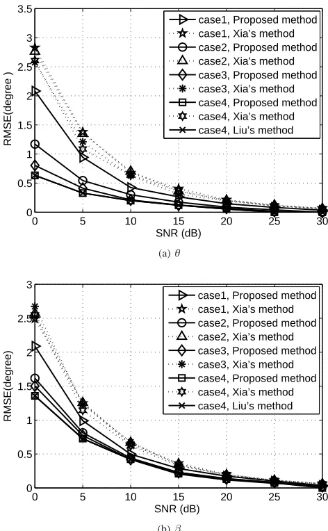
In this set of simulations, we study the performance with a varying SNR from 0dB to 30dB. There are four uncorrelated
signals from directions (60◦
,50◦), (80◦
,70◦), (100◦ ,85◦)
and (125◦
,105◦
). We consider four cases where one, two, three and four BPSK signals are considered, respectively. The number of snapshots is 1200. As shown in Fig. 5 (a) and (b), the proposed method outperforms Xia’s method in all cases because the noise subspace dimension increases by exploiting the conjugate information of the received data. Moreover, the 2-D DOA estimation performance of the proposed method improves from case 1 to case 4, and the reason for this is that the noise subspace has been extended by increasing the number of BPSK signals. Especially, for case 4 where the incoming signals are all BPSK, the proposed method is reduced to Liu’s method except that the way to construct the
new data vector ˘z is different. Therefore, in this case both
methods have the same performance.
C. Performance versus number of snapshots
The performance of the proposed method is studied in this part with the number of snapshots varying from 50 to 750. The SNR is fixed at 15 dB and the other parameters are the same as in section B. The RMSE results for the three methods are shown in Fig. 6 (a) and (b), and we can draw similar conclusions as in section B.
D. Performance versus angle separation
Now the performance of the proposed method is investigated
with the angle separation∆ of 2-D DOAs varying from5◦
to
23◦
. The SNR is fixed at 20dB and the snapshot number is 800.
Four uncorrelated signals arrive from directions (65◦
,40◦),
((65 + ∆)◦
,(40 + ∆)◦),(100◦
,75◦)and((100 + ∆)◦
,(75 +
∆)◦
). We consider three cases where one, two and three BPSK signals are present. Naturally, when angle separation is small, all methods will suffer with a high RMSE value and their performance will improve with a larger separation angle, as shown in Fig. 7 (a) and (b). Moreover, our proposed method again has outperformed Xia’s method for all three cases.
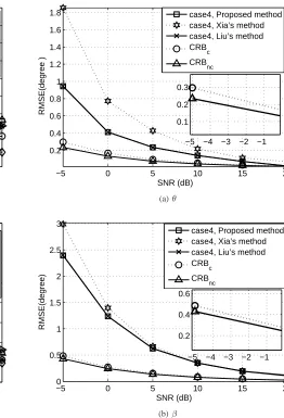
E. Deterministic CRB [28] for strictly noncircular signals versus SNR
Here, we only study the deterministic CRB with case 4 mentioned in section B where all the incoming signals are BPSK. Keeping other parameters unchanged as in simulation
B, we set the sensor number to five, and vary the SNR from
-5dB to 20dB. As shown in Fig. 8 (a) and (b), the deterministic
CRB for strictly noncircular signals denoted as CRBnc has a
lower RMSE value than the deterministic CRB for circular
signals which is denoted as CRBc at low SNRs which is in
[image:7.612.69.291.62.317.2]0 5 10 15 20 25 30 0
0.5 1 1.5 2 2.5 3 3.5
SNR (dB)
RMSE(degree )
case1, Proposed method case1, Xia’s method case2, Proposed method case2, Xia’s method case3, Proposed method case3, Xia’s method case4, Proposed method case4, Xia’s method case4, Liu’s method
(a)θ
0 5 10 15 20 25 30
0 0.5 1 1.5 2 2.5 3
SNR (dB)
RMSE(degree)
case1, Proposed method case1, Xia’s method case2, Proposed method case2, Xia’s method case3, Proposed method case3, Xia’s method case4, Proposed method case4, Xia’s method case4, Liu’s method
[image:8.612.62.298.64.446.2](b)β
Fig. 5. RMSE of versus SNR with the snapshots being 1200.
V. CONCLUSION
A generalized 2-D DOA estimation algorithm for mixed circular and non-circular signals has been proposed based on a 2-D array structure consisting of two parallel ULAs. As also demonstrated by extensive simulation results, compared to existing methods, the proposed one has three main advantages. Firstly, it can give a more accurate estimation in situations where the number of sources is within the traditional limit of high resolution methods; secondly, it can still work effectively when the number of mixed signals is larger than that of the array elements; thirdly, the paired 2-D DOAs of the proposed method can be obtained automatically without the complicated 2-D spectrum peak search and therefore has a much lower computational complexity.
APPENDIX
Here, we prove that (30) and (31) are equivalent.
Proof : The orthogonality between En and C can be ex-˘ panded as
EHn1 EHn2
C1 C2 02M×Kc
C∗1 02M×Kc C
∗
2
=0 (41)
100 200 300 400 500 600 700
0 0.5 1 1.5 2
Snapshots
RMSE(degree )
case1, Proposed method case1, Xia’s method case2, Proposed method case2, Xia’s method case3, Proposed method case3, Xia’s method case4, Proposed method case4, Xia’s method case4, Liu’s method
(a)θ
100 200 300 400 500 600 700
0.2 0.4 0.6 0.8 1 1.2 1.4 1.6 1.8 2
Snapshots
RMSE(degree)
case1, Proposed method case1, Xia’s method case2, Proposed method case2, Xia’s method case3, Proposed method case3, Xia’s method case4, Proposed method case4, Xia’s method case4, Liu’s method
(b)β
Fig. 6. RMSE of versus snapshots with the SNR fixed at 15dB.
Due to EHn1, EHn2, C1, C
∗
1, C2 and C
∗
2 are block matrices,
(41) can be rewritten in the following form
EHn2 EHn1
C∗1 C∗2 02M×Kc
C1 02M×Kc C2
=0 (42)
Applying the conjugate operation on both sides of (42), we obtain
ETn2 ETn1
C1 C2 02M×Kc
C∗1 02M×Kc C
∗
2
=0 (43)
Define E˜n =
ETn2 ETn1 H which is an orthonormal
matrix. Then (43) can be rewritten as
˜
EHnC˘ =0 (44)
SinceC is a full-column-rank matrix,˘ E˜n will also span the
noise subspace. From the uniqueness of the projection matrix onto a subspace, one can readily conclude that
P=EnEHn = ˜EnE˜ H
[image:8.612.324.561.65.448.2]6 8 10 12 14 16 18 20 22 0
0.05 0.1 0.15 0.2 0.25 0.3 0.35 0.4 0.45
Angle separation (degree )
RMSE(degree )
case1, Proposed method case1, Xia’s method case2, Proposed method case2, Xia’s method case3, Proposed method case3, Xia’s method
(a)θ
6 8 10 12 14 16 18 20 22
0.1 0.15 0.2 0.25 0.3 0.35 0.4 0.45 0.5
Angle separation (degree)
RMSE(degree)
case1, Proposed method case1, Xia’s method case2, Proposed method case2, Xia’s method case3, Proposed method case3, Xia’s method
[image:9.612.292.554.63.448.2](b)β
Fig. 7. RMSE versus angle separation with with SNR fixed at 20dB and the number of snapshots being 800.
where
EnEHn =
En1 En2
EHn1 EHn2
=
En1EHn1 En1EHn2 En2EHn1 En2EHn2
(46)
˜ EnE˜
H n =
"
˜ E∗n2
˜ E∗n1
# h
˜
ETn2 E˜Tn1
i
=
"
˜
En∗2E˜Tn2 E˜∗n2E˜Tn1 ˜
En∗1E˜Tn2 E˜∗n1E˜Tn1
#
=
"
(˜En2E˜
H n2)
∗
(˜En2E˜
H n1)
∗
(˜En1E˜
H n2)
∗
(˜En1E˜
H n1)
∗
#
(47)
Therefore, we have the following equation
En1EHn1= (En2EHn2)
∗
, (48)
which completes the proof.
REFERENCES
[1] H. Krim and M. Viberg, “Two decades of array signal processing research: the parametric approach,” IEEE Signal Processing Magazine, vol. 13, no. 4, pp. 67–94, 1996.
−5 0 5 10 15 20
0.2 0.4 0.6 0.8 1 1.2 1.4 1.6 1.8
SNR (dB)
RMSE(degree )
case4, Proposed method case4, Xia’s method case4, Liu’s method CRB
c
CRB
nc
−5 −4 −3 −2 −1
0.1 0.2 0.3
(a)θ
−50 0 5 10 15 20
0.5 1 1.5 2 2.5 3
SNR (dB)
RMSE(degree)
case4, Proposed method case4, Xia’s method case4, Liu’s method CRB
c
CRB
nc
−5 −4 −3 −2 −1
0.2 0.4 0.6
(b)β
Fig. 8. RMSE of CRB versus SNR with the snapshots being 1200.
[2] J. Liang, “Joint azimuth and elevation direction finding using cumulant,”
IEEE Sensors Journal, vol. 9, no. 4, pp. 390–398, 2009.
[3] T. Xia, Y. Zheng, Q. Wan, and X. Wang, “Decoupled estimation of 2-D angles of arrival using two parallel uniform linear arrays,” IEEE
Transactions on Antennas and Propagation, vol. 55, no. 9, pp. 2627–
2632, 2007.
[4] Q.-Y. Yin, R. Newcomb, and L.-H. Zou, “Estimating 2-D angles of arrival via two parallel linear arrays,” in Acoustics, Speech, and
Sig-nal Processing, 1989. ICASSP-89., 1989 InternatioSig-nal Conference on.
IEEE, 1989, pp. 2803–2806.
[5] H. Tao, J. Xin, J. Wang, N. Zheng, and A. Sano, “Two-dimensional direction estimation for a mixture of noncoherent and coherent signals,”
IEEE Transactions on Signal Processing, vol. 63, no. 2, pp. 318–333,
2015.
[6] H. Chen, C.-P. Hou, Q. Wang, L. Huang, and W.-Q. Yan, “Cumulants-based toeplitz matrices reconstruction method for 2-D coherent DOA estimation,” IEEE Sensors Journal, vol. 14, no. 8, pp. 2824–2832, 2014. [7] Y. Wu, G. Liao, and H.-C. So, “A fast algorithm for 2-D direction-of-arrival estimation,” Signal processing, vol. 83, no. 8, pp. 1827–1831, 2003.
[8] J. Liang and D. Liu, “Joint elevation and azimuth direction finding using L-shaped array,” IEEE Transactions on Antennas and Propagation, vol. 58, no. 6, pp. 2136–2141, 2010.
[9] G. Wang, J. Xin, N. Zheng, and A. Sano, “Computationally efficient subspace-based method for two-dimensional direction estimation with L-shaped array,” IEEE Transactions on Signal Processing, vol. 59, no. 7, pp. 3197–3212, 2011.
[image:9.612.75.406.65.449.2]estimation with propagator method,” IEEE Transactions on Antennas
and Propagation, vol. 53, no. 5, pp. 1622–1630, 2005.
[11] S. Kikuchi, H. Tsuji, and A. Sano, “Pair-matching method for estimating 2-D angle of arrival with a cross-correlation matrix,” IEEE Antennas and
Wireless Propagation Letters, vol. 5, no. 1, pp. 35–40, 2006.
[12] N. Xi and L. Liping, “A computationally efficient subspace algorithm for 2-D DOA estimation with L-shaped array,” IEEE Signal Processing
Letters, vol. 21, no. 8, pp. 971–974, 2014.
[13] J.-F. Gu and P. Wei, “Joint svd of two cross-correlation matrices to achieve automatic pairing in 2-D angle estimation problems,” IEEE
Antennas and Wireless Propagation Letters, vol. 6, pp. 553–556, 2007.
[14] Z. Ye and C. Liu, “2-D DOA estimation in the presence of mutual coupling,” IEEE Transactions on Antennas and Propagation, vol. 56, no. 10, pp. 3150–3158, 2008.
[15] F.-J. Chen, S. Kwong, and C.-W. Kok, “Esprit-like two-dimensional DOA estimation for coherent signals,” IEEE Transactions on Aerospace
and Electronic Systems, vol. 46, no. 3, pp. 1477–1484, 2010.
[16] W. Zhang, W. Liu, J. Wang, and S. L. Wu, “Computationally efficient 2-D DOA estimation for uniform rectangular arrays,” Multidimensional
Systems and Signal Processing, vol. 25, pp. 847–857, October 2014.
[17] J. Liu, Z. Huang, and Y. Zhou, “Extended 2q-music algorithm for noncircular signals,” Signal Processing, vol. 88, no. 6, pp. 1327–1339, 2008.
[18] J.-P. Delmas and H. Abeida, “Stochastic cramer-rao bound for noncir-cular signals with application to DOA estimation,” IEEE Transactions
on Signal Processing, vol. 52, no. 11, pp. 3192–3199, 2004.
[19] J. Steinwandt, F. Roemer, M. Haardt, and G. Del Galdo, “R-dimensional esprit-type algorithms for strictly second-order non-circular sources and their performance analysis,” IEEE Transactions on Signal Processing, vol. 62, no. 18, pp. 4824–4838, 2014.
[20] H. Abeida and J.-P. Delmas, “Efficiency of subspace-based doa estima-tors,” Signal Processing, vol. 87, no. 9, pp. 2075–2084, 2007. [21] H. Abeida and J.-P. Delmas, “Music-like estimation of direction of
ar-rival for noncircular sources,” IEEE Transactions on Signal Processing, vol. 54, no. 7, pp. 2678–2690, 2006.
[22] M. Haardt and F. Romer, “Enhancements of unitary esprit for non-circular sources,” in Acoustics, Speech, and Signal Processing, 2004.
Proceedings.(ICASSP’04). IEEE International Conference on, vol. 2.
IEEE, 2004, pp. ii–101.
[23] Z. Huang, Z. Liu, J. Liu, and Y. Zhou, “Performance analysis of music for non-circular signals in the presence of mutual coupling,” IET radar,
sonar & navigation, vol. 4, no. 5, pp. 703–711, 2010.
[24] P. Charg´e, Y. Wang, and J. Saillard, “A non-circular sources direction finding method using polynomial rooting,” Signal Processing, vol. 81, no. 8, pp. 1765–1770, 2001.
[25] H. Abeida and J.-P. Delmas, “Gaussian cramer-rao bound for direction estimation of noncircular signals in unknown noise fields,” IEEE
Trans-actions on Signal Processing, vol. 53, no. 12, pp. 4610–4618, 2005.
[26] J. Liu, Z. Huang, and Y. Zhou, “Azimuth and elevation estimation for noncircular signals,” Electronics letters, vol. 43, no. 20, pp. 1117–1119, 2007.
[27] L. Gan, J.-F. Gu, and P. Wei, “Estimation of 2-D DOA for noncircular sources using simultaneous svd technique,” IEEE Antennas and Wireless
Propagation Letters, vol. 7, pp. 385–388, 2008.
[28] F. Roemer and M. Haardt, “Efficient 1-D and 2-D DOA estimation for non-circular sourceswith hexagonal shaped espar arrays,” in Acoustics,
Speech and Signal Processing, 2006. ICASSP 2006 Proceedings. 2006 IEEE International Conference on, vol. 4. IEEE, 2006, pp. IV–IV. [29] F. Gao, A. Nallanathan, and Y. Wang, “Improved music under the
coexistence of both circular and noncircular sources,” IEEE Transactions
on Signal Processing, vol. 56, no. 7, pp. 3033–3038, 2008.
[30] A. Liu, G. Liao, Q. Xu, and C. Zeng, “A circularity-based DOA estimation method under coexistence of noncircular and circular sig-nals,” in Acoustics, Speech and Signal Processing (ICASSP), 2012 IEEE
International Conference on. IEEE, 2012, pp. 2561–2564.
[31] Z.-M. Liu, Z.-T. Huang, Y.-Y. Zhou, and J. Liu, “Direction-of-arrival estimation of noncircular signals via sparse representation,” IEEE
Trans-actions on Aerospace and Electronic Systems, vol. 48, no. 3, pp. 2690–
2698, 2012.
[32] P. J. Schreier, “Bounds on the degree of impropriety of complex random vectors,” IEEE Signal Processing Letters, vol. 15, pp. 190–193, 2008. [33] J. P. Delmas and H. Abeida, “Asymptotic distribution of circularity