A personalized-model-based central aortic pressure estimation method

(1)

White Rose Research Online URL for this paper:

http://eprints.whiterose.ac.uk/108846/

Version: Accepted Version

Article:

Jiang, S, Zhang, Z-Q orcid.org/0000-0003-0204-3867, Wang, F et al. (1 more author)

(2016) A personalized-model-based central aortic pressure estimation method. Journal of

Biomechanics, 49 (16). pp. 4098-4106. ISSN 0021-9290

https://doi.org/10.1016/j.jbiomech.2016.11.007

© 2016 Elsevier Ltd. Licensed under the Creative Commons

Attribution-NonCommercial-NoDerivatives 4.0 International

http://creativecommons.org/licenses/by-nc-nd/4.0/

[email protected] https://eprints.whiterose.ac.uk/

Reuse

Unless indicated otherwise, fulltext items are protected by copyright with all rights reserved. The copyright exception in section 29 of the Copyright, Designs and Patents Act 1988 allows the making of a single copy solely for the purpose of non-commercial research or private study within the limits of fair dealing. The publisher or other rights-holder may allow further reproduction and re-use of this version - refer to the White Rose Research Online record for this item. Where records identify the publisher as the copyright holder, users can verify any specific terms of use on the publisher’s website.

Takedown

If you consider content in White Rose Research Online to be in breach of UK law, please notify us by

(2)

A Personalized-Model-based Central Aortic

1

Pressure Estimation Method

2

Sheng Jiang

1

, Zhi-Qiang Zhang

2

Fang Wang

3

and Jian-Kang Wu

4

3

1

China Academy of Electronics and Information Technology,Beijing,China

4

2

School of Electronics and Electrical Engineering, University of Leeds, UK

5

3

Division of Cardiology, Beijing Hospital, Beijing, China

6

4

Department of Electrical Engineering, University of Chinese Academy of Sciences, Beijing, China

7

Email:[email protected]

8

Abstract

9

Central Aortic Pressure (CAP) can be used to predict cardiovascular structural damage and cardiovascular events, and the

10

development of simple, well-validated and non-invasive methods for CAP waveforms estimation is critical to facilitate the routine

11

clinical applications of CAP. Existing widely applied methods, such as generalized transfer function (GTF-CAP) method and

N-12

Point Moving Average (NPMA-CAP) method, are based on clinical practices, and lack a mathematical foundation. Those methods

13

also have inherent drawback that there is no personalisation, and missing individual aortic characteristics. To overcome this pitfall,

14

we present a personalized-model-based central aortic pressure estimation method (PM-CAP)in this paper. This PM-CAP has a

15

mathematical foundation: a human aortic network model is proposed which is developed based on viscous fluid mechanics theory

16

and could be personalized conveniently. Via measuring the pulse wave at the proximal and distal ends of the radial artery, the least

17

square method is then proposed to estimate patient-specific circuit parameters. Thus the central aortic pulse wave can be obtained

18

via calculating the transfer function between the radial artery and central aorta. An invasive validation study with 18 subjects

19

comparing PM-CAP with direct aortic root pressure measurements during percutaneous transluminal coronary intervention was

20

carried out at the Beijing Hospital. The experimental results show better performance of the PM-CAP method compared to the

21

GTF-CAP method and NPMA-CAP method, which illustrates the feasibility and effectiveness of the proposed method.

22

Index Terms

23

Central Aortic Pressure, Blood Fluid Dynamics, Human Artery Model, Transfer Function.

24

I. INTRODUCTION

25

Central Aortic Pressure (CAP) has been widely applied to predict the cardiovascular structural damage and cardiovascular 26

events(? _{). Traditionally, Blood Pressure (BP) measured over the brachial artery using a sphygmomanometer has been used}

27

to predict such damage and events directly, but the measured brachial BP can’t always accurately represent the corresponding 28

pressure in the aorta due to the influence of many factors, such as arterial stiffness, age, heart rate, body height, sex, and drug 29

therapies. All these factors can affect the relationship between brachial pressure and CAP( ? _{). In recent years, the standard}

30

method for CAP measurement is the direct measurement of aortic root pressures using a pressure transducer introduced into 31

the aortic root at the time of percutaneous transluminal coronary intervention( ? _{). This method can provide accurate CAP}

32

measurement for individuals, but it is invasive and unsuitable for routine clinical practices; therefore, the development of 33

simple, well-validated methods for non-invasive CAP derivation is critical to facilitate routine clinical applications. 34

Thus far, some ad-hoc methods have been proposed for non-invasive CAP estimation. For example, ? _{proposed to use}

35

electrical impedance tomography (EIT) to measure the blood pressure pulses directly within the descending aorta, but it 36

required at least 32 impedance electrodes placed around the chest at the level of the axilla, which prevented it from the 37

routine clinical practice. In contrast, the Generalized Transfer Function (GTF) method, which applies a transfer function for 38

CAP derivation and related aortic hemodynamic indices extraction, has attracted extensive research interest in the past decade 39

( ? ? _{). Although there are already several commercial products, such as SphygmoCorand HEM-9000AI, which are widely}

40

used in the clinical environment, how to determine the transfer function, particularly the specific transfer function for different 41

subjects remains a challenge. ? _{further simplified the idea of a general function and proposed a simple N-Point Moving}

42

Average (NPMA), mathematically a low pass filter, to non-invasively derive CAP from the radial artery pressure waveform. 43

Both the GTF-CAP or NPMA-CAP methods can be used for noninvasive assessment of central aortic pressure indices, but they 44

ignore the individual differences in terms of blood viscosity, fluid inertia and arterial compliance, which may cause significant 45

CAP errors. 46

To take the individual differences into consideration and improve the CAP estimation accuracy, it is critical to model the 47

arteries. In general, the arteries can be modeled as a 0D-model, 1D-model, 2D-model and 3D-model( ? _{). The 3D and 2D}

48

models are widely applied for the analysis of local blood flow. For example, ? _{applied a 3D-model to study blood flow}

49

circulation in intracranial arterial networks. ?_{explored the pulsating turbulent phenomena in stenotic vessels. A 1D-model of}

50

the blood flow in deformable vessels has been proven to be a simple and effective approach to simulate the hemodynamics 51

of the vascular system, which has been widely used for systematic arterial network modeling(? _{). For example,} ? _applied

(3)

[image:3.595.155.441.80.312.2]

TABLE I: The subjects detailed information

(Sex,Age,Systolic blood pressure,Diastolic blood pressure and Diabetes)

Sex Age SBP(mmHg) DBP(mmHg) Diabetes

No.1 F 85 136 58 No

No.2 M 60 117.4 64.5 Yes

No.3 M 62 112.7 65.1 Yes

No.4 F 59 128.6 57.6 No

No.5 M 57 125.6 47.8 Yes

No.6 F 70 107.7 69.5 Yes

No.7 M 71 129.9 63 No

No.8 M 63 116.4 81.2 Yes

No.9 F 55 152.4 59.8 Yes

No.10 M 62 155.4 73.8 No

No.11 F 56 137.3 62.5 Yes

No.12 M 66 117.5 68.1 Yes

No.13 M 63 106.5 53.3 Yes

No.14 F 70 144.6 67.9 Yes

No.15 F 73 146 67.4 No

No.16 M 58 142.3 78.4 Yes

No.17 M 54 133.5 71.9 Yes

No.18 F 62 101.9 59.2 No

Mean±_SD _63.7±_7.7 _128.4±_16.2 _65.0±_8.5

Range 56%(M) 54∼₈₅ _101.9∼_155.4 _47.8∼_81.2 _66.7%(Y)

a 1D-model to compare the pressure and flow wave propagation in conduit arteries against a well-defined experimental 1:1 53

replica of the human arterial tree, which consisted of 37 silicone branches representing the largest central systemic arteries in 54

the human. ?_{proposed a simple lumped parameter model for the heart and showed how it could be coupled numerically with}

55

a 1D model of the arteries. However, 1D-models requires defined of vessel parameters, such as vessel radius, blood density 56

and wall thickness, in advance which can’t be acquired non-invasively. Unlike a 1D-model which reduces the vessel space 57

dependence to the vessel axial coordinate only, 0D-models discretize the space dependence by splitting the cardiovascular 58

system into a set of compartments, and uses an equivalent electric circuit to describe the arbitrary length and structure of blood 59

vessels( ?? _{), which can significantly reduce the complexity of the vascular modeling, but it can’t describe the geometrical}

60

structure of arteries network in the 0D-model. 61

Considering the state-of-the-art for non-invasive CAP estimation and vascular system modeling, we present a personalized-62

model-based central aortic pressure estimation method (PM-CAP)in this paper. The main contributions of the paper are: 63

• Personalized artery network model: The vessels are mathematically modeled based on hydrodynamics with the continuity

64

and the momentum equations. This model method ismore thorough than the Windkessel model method.The models 65

parameters can be personalized: via measuring the pulse wave at the proximal and distal ends of the radial artery, the 66

least square method is then proposed to estimate the model parameters. 67

• Personalized transfer function and CAP waveform estimation: a Subject-specific ascending aorta-radial artery transfer

68

function can then be acquired to obtain the continuous central artery blood pressure waveform. 69

An invasive validation study with 18 subjects comparing PM-CAP with direct aortic root pressure measurements during 70

percutaneous transluminal coronary intervention was carried out at the Beijing Hospital. The experimental results have shown 71

accurate CAP estimations can be acquired with regard to the invasive measurements for all the subjects, which illustrates the 72

feasibility and effectiveness of the proposed method. 73

The remainder of the paper is organized as follows. Section II presents the viscous fluid mechanics based arteries model,the 74

patient-specific parameter estimation and CAP estimation. Experimental results and conclusion are then provided in Section 75

III and IV. 76

II. PM-CAPMETHOD

77

A. Data Acquisition

78

18 subjects (10 males, 8 females) were recruited (Table I). All volunteers gave written informed consent approved by the 79

Institutional Review Board at Beijing Hospital before participating. Direct aortic root pressure waveforms were collected during 80

percutaneous transluminal coronary intervention by inserting a 6FR angiography catheter (Cordis Corporation) into the right 81

radial artery, and the catheter was connected to the commercial Mac-Lab hemodynamic recording system(GE Healthcare) . 82

Meanwhile, pulse waveforms at the proximal and distal ends of the radial artery were also measured by catheter, which is 83

(4)

B. Human Arteries Modeling

85

Human arteries are composed of finite but very small vessels and they can be divided into large arteries and small arteries 86

according to the radius. In this section, we will introduce these two types of arteries separately. 87

1) Large arteries: As shown in the Fig.2, any large arteryΩl_{of length}_l _{can be modeled as}_N _{finite but very small vessels}

88

Ωl,₁∆l, Ωl,₂∆l_{· · ·} and Ωl,_N∆l with the same properties; therefore, we can assume cross-sectional area A0; blood viscosity, η, 89

blood density ρ, vascular thickness h0, Young’s modulus E, average blood flow Qˆ(t)and average blood pressure Pˆ(t) are 90

constant. Thus according to Equation (34) the fluid dynamics equations of large artery can then be simplified as: 91

  

 

CdP(t)

dt +Q(t, xe)−Q(t, xs) = 0 LdQ(t)

dt +RQ(t) +P(t, xe)−P(t, xs) = 0

(1)

where C = 2l√A0

β is arterial compliance, L = ρl/A0 is the fluid inertia, R =

8ηl πr4

0 is blood resistance. However, similar

92

equations can also be found in the analysis of electric circuits, thus we can simulate the flow in the vascular system based on 93

analog electric circuits. In the electric network analogy, the blood flowQand blood pressure P are equivalent to the current 94

and voltage, while arterial compliance, blood inertia and blood resistance correspond to capacitance, inductance and resistance; 95

therefore, the corresponding circuit can be derived as shown in Fig.3. 96

2) Small arteries: Similar to the large arteries, we can define a small artery as ΩM _as _N _{finite but very small vessels}

97

Ω₁M,∆l,Ω₂M,∆l_{· · ·} andΩM,_N ∆l, then we obtain the similar fluid dynamics equations as: 98

   

  

CMdPM(t)

dt +Q

M₍_{t, x}

e)−QM(t, xs) = 0

LMdQM(t)

dt +R

M_QM₍_t₎₊_PM₍_{t, x}

e)−PM(t, xs) = 0

(2)

whereCM _{is the compliance,}_LM _{is the fluid inertia,}_RM _{is the blood resistance,}_QM _{is the blood flow and} _PM _{is the blood}

99

pressure. Since dP

M

(t)

dt and dQM(t)

dt are very small in small arteries, they can be ignored, thus we can simplify the above

100

equations to: 101

(

QM₍_{t, x}

e)−QM(t, xs) = 0

RM_QM₍_t_{) +}_PM₍_{t, x}

e)−PM(t, xs) = 0.

(3)

Similarly, the corresponding circuit can be obtained as shown in Fig.4. In practice, we always take the resistanceRM _{in small}

102

arteries as the peripheral resistance, and use symbolRPM _{to represent it.}

103

C. Human Arteries Network Model

104

Human body has 55 large arteries and 28 small arteries. This division was originally introduced by ? _{and the data of}

105

diameter, length , wall, thickness and Youngs modulus of 55 largest arteries was introduced by ?_{. Using the electric circuit}

106

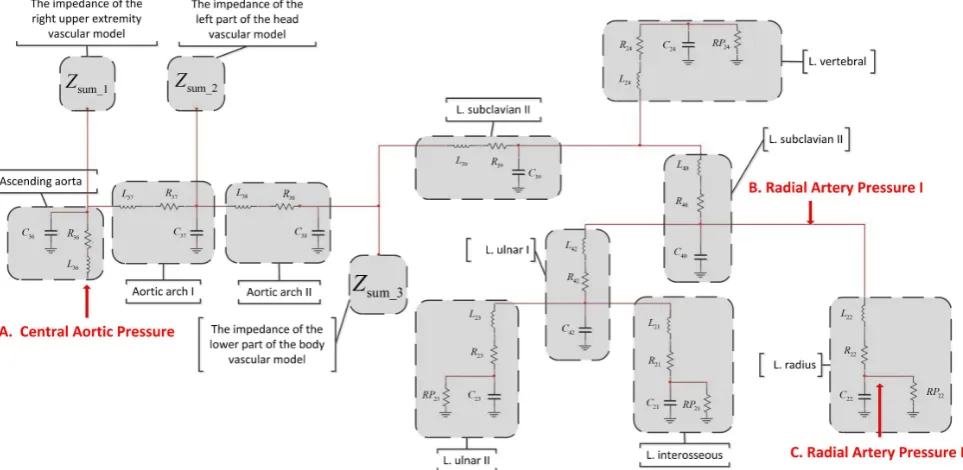
in Fig.3 to represent large arteries and the electric circuit in Fig.4 to represent small arteries, the human arterial network can 107

be abstracted as a network of electric circuits consisting of capacitance, inductance and resistance, as shown in Fig.5. Due to 108

space constrictions, here we only present the circuit between the left radial artery and ascending aorta, the whole body circuit 109

given at the end of this paper(Appendix B). To estimate the BP at point Afrom the BP measurement at pointB andC, the 110

circuit parameters need to be estimated first. 111

D. Patient-Specific Parameters Estimation

112

To determine the patient-specific parameters for the human artery network as shown in Fig.5, we need to estimate: 1)RPi,

113

wherei= 1,2,· · ·28, 2)Lj,Cj andRj, wherej= 1,2· · ·55. Via measuring the pulse wave of the proximal and distal ends

114

of the radial artery: P22(t, xs)andP22(t, xe), we will introduce how to estimate them separately.

115

1) Estimate Peripheral ResistancesRPi: On the basis of 0D theory, R+RP =P/CO (P is the average central aortic

116

pressure, CO is cardiac output, R is total large artery resistance, and RP is total small artery resistance). Then we have 117

2 assumption that: (1)the average BP at central artery is equal to the average BP at the proximal end of radial artery [1]; 118

(2)because of the radius of small arteries is less then the radius of large arteries, theRP is widely larger then theR ( see the 119

expression forR ,Equation (18)), ignore the R. ThenR+RP =P/CO is simplified to: 120

RP ≈ P¯22_CO(xs) (4)

whereP¯22(xs)is the average BPatthe proximal end of radial artery over periodT, which can be calculated as

121

¯

P22(xs) =

1

T

Z T 0

(5)

CO is the cardiac output, which is given as?_:

122

CO= 17

K2(P

s

22−P22d) (6)

wherePs

22 andP22d are the measured systolic and diastolic blood pressure at the proximal end of radial artery respectively, 123

and K is the pulse contour characteristic value as ?

124

K= P¯22(xs)−P

d

22

Ps

22−P22d

. (7)

The relationship betweenRPi and the total peripheral resistanceRP can be written as:

125 1 RPi = 1 RP − X k 1 RPk (8)

wherek= 1,2,_{· · ·}28andk₆=i. Denote the ratio wRP

k as RPRPk, then we can get

126

1

RPi

= RP

1−P

k RPRPk

= RP

1₋P

kwkRP

. (9)

Here,the ratio wRP

k can be assumed to be constant for different subjects to simplify the derivation process, and they can be

127

acquired in advance?_.

128

2) Estimate Left Radial Artery Model Parameters(The least squares method):R22,C22and L22: To simplify the analysis, 129

the left radial artery model is shown separately in Fig.6, where R22,L22,C22 are its resistance, inductance and capacitance, 130

respectively;P22(t, xs),P22(t, xe),Q22(t, xs)andQ22(t, xe)are blood pressures and flows in the both ends of radial artery

131

respectively. 132

From the radial artery model shown in Fig.6, we can obtain the following equations: 133 134           

P22(t, xe) =Q22(t, xe)RP22

dP22(t, xe)

dt =

Q22(t, xs)−Q22(t, xe)

C22 dQ22(t, xs)

dt =

P22(t, xs)−P22(t, xe)−Q22(t, xs)·R22

L22

(10)

135

get the below equation from Equation (10): 136

L22C22RP22

d2_Q

22(t, xe)

dt2 +(L22+R22C22RP22)

·dQ22_dt(t, xe)+(RP22+R22)Q22(t, xe)=P22(t, xs).

(11)

Take anyN sets of measurementsP22(t, xs),P22(t, xe)from t=t1, t2· · ·tN, we can have

137

P22,N =HNθ (12)

where 138

P22,N =



   

P22(t1, xs)

P22(t2, xs)

.. . P22(tN, xs)

     , (13) 139

θ= [θ1, θ2, θ3]T

= [L22C22P R22, L22+R22C22P R22, RP22+R22]T

(14)

and 140

HN =

      d2

Q22(t1,xe)

dt2

dQ22(t1,xe)

dt Q22(t1, xe) d2

Q22(t2,xe)

dt2

dQ22(t2,xe)

dt Q22(t2, xe)

..

. ... ...

d2

Q22(tN,xe)

dt2

dQ22(tN,xe)

dt Q22(tN, xe)

      (15)

so we can get θˆas: 141

ˆ

θ= (HT

(6)

ThusR22,C22 andL22can be calculated as: 142

     

    

R22= ˆθ3−RP22

C22= ˆ

θ2RP22+ q

(ˆθ2RP22)2−4ˆθ1R22(RP22)2 2R22(RP22)2

L22= ˆθ2−C22R22RP22.

(17)

The solution about estimating left radial artery model parameters is that: Firstly, the peripheral resistance of radial artery 143

RP22could be calculated by equation (4) to (9). Secondly, the blood flow at the end of radial arteryQ22(t, xe)in equation(15)

144

could be calculated by the first equation of equation set (10): Q22(t, xe) = P22(t, xe)/RP22 . It means that, we use the 145

pressure of proximal and distal ends of radial artery :P22(t, xs)andP22(t, xe)to estimate theR22 ,C22 ,L22 of radial artery 146

by equation (16) and (17). 147

3) Estimate Other large Arteries Parameters:Rj,Cj andLj : For anyjth(j= 1,2,3· · ·,55)large artery in the Fig.5, the

148

Cj,Rj andLj can be defined as?:

149

Cj =

2lj

p

A0,j

βj

Rj =

8ηlj

πr4

i

Lj =

ρlj

A0,j

.

(18)

where 150

βj=

√_πh

0,jEj

(1-υ2₎_A 0,j

. (19)

Define 151

ωA

j =A0,j/A0,22

ωlj=lj/l22

ωjr=rj/r22

ωh

j =h0,j/h0,22

ωEj =Ej/E22

(20)

Then we can have: 152

         

        

Cj =C22·

ljpAjβ22

l22√A22βj

=C22ω

l j(

q

ωA j)3

ωh jωjE

Rj =R22

lj/(rj)4

l22/(r22)4

=R22ωlj/(ωrj)

4

Lj =L22 lj/A0,i

l22/A0,22

=L22ωjl/ωjA.

(21)

Similar towRP

i ,ωjA,ωlj,ωjr,ωhj andωEj are also constant for different subjects, and they can be acquired in advance(?).

153

E. CAP Estimation

154

Once all the parameters in the Fig.5 are known, it is straightforward to calculate the impulse response functionH(t)between 155

the radial arterial blood pressureP22(t, xe)and central aortic blood pressureCAP(t)(? ), and the central aortic pressure can

156

then be estimated as 157

CAP(t) =H(t)_⊗P22(t, xe) (22)

where_⊗represents the convolution operation. 158

III. EXPERIMENTALRESULTS ANDDISCUSSION

159

To better illustrate the performance of our method, we compared the estimated CAP with the ground-truth measured from 160

the catheter during percutaneous transluminal coronary intervention. For analysis purpose, the comparison between our method 161

(7)

A. CAP waveform estimation results

163

Central aortic waveforms contain valuable cardiovascular information, for example, the rising phases of the waveforms 164

reflects the myocardial contractility, while the descending phases illustrate the timing of aortic valve closure; therefore, it is 165

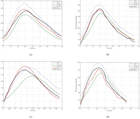
critical to recover the CAP waveforms. In our first experiment, parameter values of the radial artery and the blood pressure 166

waveforms of the central artery were estimated, which are given in the Table II and Fig.7. In the Fig.7, the black solid lines 167

indicate the direct invasive measurements as the ground-truth, the red dashed lines represent our estimations, while the blue 168

dotted lines and green dotted-dashed lines are the estimated waveforms by the GTF-CAP and NPMA-CAP, respectively. 169

The GTF-CAP and NPMA-CAP measures were obtained by collected the blood pressure at the distal end of the radial artery 170

by inserting a 6FR angiography catheter (Cordis Corporation) ,which is connected to the commercial Mac-Lab hemodynamic 171

recording system(GE Healthcare) ,into the right radial artery at Beijing Hospital. The GTF method (?_{) to estimate the central}

172

artery pressure : (1)Get the general transfer function which is calculated by a large number of clinical experiment data (?_):

173

radial artery pressureaortic artery pressure. (2)Blood pressure÷GTF to estimate the central artery pressure. Thirdly, we used 174

NPMA(?_{) method to estimate the central artery pressure: use n-point moving average method which acts as a low pass filter}

175

to smooth collected blood pressure data( n=samplingf requency/4, the value is 256 in this article). 176

As we can see from the Fig.7, it is obvious that our proposed method can get more accurate CAP waveforms for different 177

subjects compared to the GTF-CAP and NPMA-CAP methods. The main reason is we estimated subject-specific parameters in 178

our method, which could handle the individual differences ignored by both GTF-CAP and NPMA-CAP methods. As shown in

TABLE II: The parameter values of the radial artery subjects. (the oldest and youngest males and females)

ID L C R RP

(mmhg·_sec2_/ml₎₍_ml/mmhg₎₍_mmhg·_sec/ml₎₍_mmhg·_sec/ml₎

1(oldest female) 0.0482 0.0029 2.988 79.95

7(oldest male) 0.0248 0.0036 0.839 43.02

5(youngest male) 0.0936 0.0012 2.402 54.06

9(youngest female) 0.0121 0.0011 4.076 62.57

179

the Table II, it is evident that there are significant artery parameters differences for subjects, and ignorance of such individual 180

differences should be avoided during the CAP estimation. Although there are no ground-truth values for the artery parameters, 181

we insist it is still worthwhile to take the individual differences into consideration and try to get more accurate CAP waveform 182

estimation. The above qualitative analysis has shown that the proposed CAP estimation method can significantly improve the 183

accuracy of the central arterial waveforms over the existing non-invasive methods. To further illustrate the strength of the 184

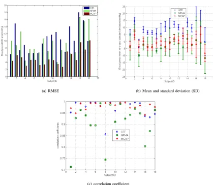
proposed method over the GTF-CAP and NPMA-CAP methods, quantitative analysis was also conducted. Here, root-mean-185

square error(RMSE)mean error and standard deviation, and correlation coefficient were used as the evaluation standards: the 186

estimated CAP and invasive measured CAP are time-varying waveforms, then we sampled 150 data points of them by 15Hz 187

frequency and subtract a point-by-point value of computed method from measured value to get errors. Lastly, calculate the 188

root-mean-square error, mean error, standard deviation and correlation coefficient. Results are shown in the Fig.8(a), Fig.8(b), 189

and Fig.8(c) respectively. As we can see from the figures, our method can achieve the smallest RMSE and high correlation 190

coefficient values for all the subjects. We also noticed the correlation coefficient values of the GTF-CAP methods are slightly 191

better than those of our method for some certain subjects, but the differences are very small and the RMSE of GTF-CAP are 192

much larger for those subjects. It illustrates that the overall performance of our method is better than those of GTF-CAP and 193

NPMA-CAP methods. 194

B. Systolic and diastolic blood pressure estimation results

195

Since the central aortic systolic and diastolic blood pressure are important indicators to measure the level of high blood 196

pressure, we also statistically analyzed the central systolic blood pressure and diastolic blood pressure as shown in the Fig.9. 197

The average errors for central aortic systolic blood pressure estimation are1.4165mmHg,6.4140mmHg and7.7991mmHg

198

for our method, NPMA-CAP and GTF-CAP, respectively, while the standard deviations of the errors are 5.8558mmHg, 199

8.1155mmHg and8.5936mmHg. The average errors for central aortic diastolic blood pressure estimation are2.1413mmHg, 200

9.4160mmHg and3.7646mmHg for our method, NPMA-CAP and GTF-CAP, respectively, while the standard deviations of 201

the errors are3.6420mmHg,4.3795mmHgand4.2777mmHg. It is evident that our proposed method can achieve the most 202

accurate and stable systolic and diastolic blood pressure estimations, and they are also consistent with the standard of the 203

Association for the Advancement of Medical Instrumentation (mean error less than 5 mmHg and standard deviation less than 204

8mmHg)(? _).

205

C. Discussion

206

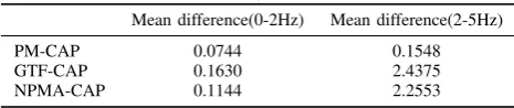
Above subsections show that PM-CAP method could estimate more accurate CAP waveform for different subjects compared 207

(8)

them (Table III). It shows that the error of PM-CAP transfer function0-5Hz is less than the errors of GTF-CAP transfer 209

function and NPMA-CAP transfer function. ?_{tell us that the power spectral density of blood pressure wave mainly distribute}

210

in the 0-5 Hz. Obviously, the main reason that PM-CAP method is more accurate than other two method is PM-CAP method 211

used subjected-specific parameters.Then the transfer function between CAP(central aortic pressure) to RAP(radial artery blood 212

[image:8.595.179.412.141.190.2]

pressure) of different subjects is personalized and more close to real transfer function. 213

TABLE III: Error Analysis of Transfer Function

Mean difference(0-2Hz) Mean difference(2-5Hz)

PM-CAP 0.0744 0.1548

GTF-CAP 0.1630 2.4375

NPMA-CAP 0.1144 2.2553

However, there are also some certain errors between our estimations and the direct invasive measurements. 214

The experiment uses invasive methods to obtain radial artery blood pressure for checking the validity of the artery model. 215

In general application scenario, we can use the pressure sensor to collect non-invasive radial arterial blood pressure waveform 216

, and use korotkoff sounds method to obtain radial artery blood pressure for calibrating the blood pressure waveform. The 217

korotkoff sounds method has difficult to obtain the accurate blood pressure, which will affect the accuracy of the pressure 218

value estimation, but this does not affect the accuracy of waveform estimation. 219

Although we have tried our best in the experiment to synchronize all the measurements, there was still some delay between 220

the pulse waves of the proximal and distal ends of the radial artery, which caused the errors in the model parameters estimation 221

and thus the error in the CAP waveform estimations. Meanwhile, to simplify the derivation and make the model computable, 222

we have made some approximations in the arteries network modeling and assumedwRP

i ,ωAj,ωjl,ωrj,ωhj andωjEwere constant

223

for different subjects. In normal condition, such assumption is valid and robust. However, such proportional constants may/may 224

not change duo external stimulations,such as drugs, which needs to be further verified. Due to the experimental constraints for 225

this pilot study, we didn’t take such condition into consideration. In the near future, when we carry out large scale studies, 226

we will explore the robustness of such assumption, and more rigorous tests on more subjects under different situations will be 227

carried out. 228

IV. CONCLUSION

229

In this paper, we present a personalized-model-based central aortic pressure estimation method (PM-CAP) (PM-CAP).PM-230

CAP has mathematical foundation: a novel human aortic network model is proposed and developed based on viscous fluid 231

mechanics theory. Via measuring the pulse wave of the proximal and distal ends of the radial artery, the least square method 232

was then proposed to estimate the patient-specific circuit parameters. Thus the central aortic pulse wave was then obtained 233

via calculating the transfer function between radial artery and central aortic. An invasive validation study with 18 subjects 234

comparing M-CAP with direct aortic root pressure measurements during coronary intervention were carried out at the Beijing 235

Hospital. The experimental results have shown better performance of PM-CAP method compared to the GTF-CAP method and 236

NPMA-CAP method, which illustrated the feasibility and effectiveness of the proposed method. In the future, more subjects’ 237

data will be collected and analyzed to further evaluate the proposed method. The exploration the relationship between the blood 238

vessel parameters and cardiovascular disease will also be carried out. [Conflict of interest]The authors declared that they have 239

no conflicts of interest to this work. We declare that we do not have any commercial or associative interest that represents a 240

conflict of interest in connection with the work submitted 241

[Conflict of interest]The authors declared that they have no conflict of interest to this work. We declare that we do not have 242

any commercial or associative interest that represents a conflict of interest in connection with the work submitted. 243

REFERENCES

244

Alpert B, Friedman B, Osborn D. Aami blood pressure device standard targets home use issues. Home Healthcare Horizons 245

2010;:69–72. 246

Chen CH, Nevo E, Fetics B, Pak PH, Yin FCP, Maughan WL, Kass DA. Estimation of central aortic pressure waveform 247

by mathematical transformation of radial tonometry pressure. validation of generalized transfer function. Circulation 248

1997;95(7):1827–36. 249

Dorf RC, Bishop RH. Modern control systems. Pearson, 2011. 250

Fetics B, Nevo E, Chen C, Kass D. Parametric model derivation of transfer function for noninvasive estimation of aortic 251

pressure by radial tonometry. Biomedical Engineering, IEEE Transactions on 1999;46(6):698–706. 252

Formaggia L, Lamponi D, Tuveri M, Veneziani A. Numerical modeling of 1d arterial networks coupled with a lumped 253

parameters description of the heart. Computer methods in biomechanics and biomedical engineering 2006;9(5):273–88. 254

Formaggia L, Quarteroni AM, Veneziani A. Cardiovascular Mathematics: Modeling and simulation of the circulatory system. 255

(9)

Grinberg L, Cheever E, Anor T, Madsen J, Karniadakis G. Modeling blood flow circulation in intracranial arterial networks: 257

a comparative 3D/1D simulation study. Annals of biomedical engineering 2011;39(1):297–309. 258

Hopcroft MA, Nix WD, Kenny TW. What is the Young’s Modulus of silicon? Microelectromechanical Systems, Journal of 259

2010;19(2):229–38. 260

Luo ZC, Zhang S, Yang YM. Pulse Wave Engineering Analysis and Clinical Application. Beijing: Science Press, 2006. 261

Matthys K, Alastruey J, Peir´o J, Khir A, Segers P, Verdonck P, Parker K, Sherwin S. Pulse wave propagation in a model 262

human arterial network: Assessment of 1-D numerical simulations against in vitro measurements. Journal of biomechanics 263

2007;40(15):3476–86. 264

O’Rourke MF, Seward JB. Central arterial pressure and arterial pressure pulse: new views entering the second century after 265

korotkov. In: Mayo Clinic Proceedings. Elsevier; volume 81; 2006. p. 1057–68. 266

Reymond P. Pressure and Flow Wave Propagation in Patient-Specific Models of the Arterial Tree. Ph.D. thesis; ´ECole 267

Polytechnique F ´ED ´ERale De Lausanne; 2011. 268

Reymond P, Merenda F, Perren F, R¨ufenacht D, Stergiopulos N. Validation of a one-dimensional model of the systemic arterial 269

tree. American Journal of Physiology-Heart and Circulatory Physiology 2009;297(1):H208–22. 270

Rłha K, Benes R. Testing of methods for artery section area detection 2011;. 271

Riha K, Chen P, Fu D. Detection of artery section area using artificial immune system algorithm. In: Proceedings of the 7th 272

conference on Circuits, systems, electronics, control and signal processing. 2008. p. 46–52. 273

Sol`a J, Adler A, Santos A, Tusman G, Sipmann FS, Bohm SH. Non-invasive monitoring of central blood pressure by electrical 274

impedance tomography: first experimental evidence. Medical & biological engineering & computing 2011;49(4):409–15. 275

Stergiopulos N, Meister JJ, Westerhof N. Simple and accurate way for estimating total and segmental arterial compliance: the 276

pulse pressure method. Annals of biomedical engineering 1994;22(4):392–7. 277

Stergiopulos N, Young D, Rogge T. Computer simulation of arterial flow with applications to arterial and aortic stenoses. 278

Journal of biomechanics 1992;25(12):1477–88. 279

Tsanas A, Goulermas J, Vartela V, Tsiapras D, Theodorakis G, Fisher A, Sfirakis P. The windkessel model revisited: A 280

qualitative analysis of the circulatory system. Medical engineering & physics 2009;31(5):581–8. 281

Varghese SS, Frankel SH. Numerical modeling of pulsatile turbulent flow in stenotic vessels. Transactions-American Society 282

Of Mechanical Engineers Journal Of Biomechanical Engineering 2003;125(4):445–60. 283

Wang J, Parker K. Wave propagation in a model of the arterial circulation. Journal of biomechanics 2004;37(4):457–70. 284

Westerhof N, Bosman F, De Vries CJ, Noordergraaf A. Analog studies of the human systemic arterial tree. Journal of 285

biomechanics 1969;2(2):121–43. 286

Westerhof N, Lankhaar J, Westerhof B. The arterial windkessel. Medical and Biological Engineering and Computing 287

2009;47(2):131–41. 288

Williams B, Lacy P, Thom S, Cruickshank K, Stanton A, Collier D, Hughes A, Thurston H, ORourke M, et al. Differential 289

impact of blood pressure–lowering drugs on central aortic pressure and clinical outcomes. Circulation 2006;113(9):1213–25. 290

Williams B, Lacy P, Yan P, Hwee C, Liang C, Ting C. Development and validation of a novel method to derive central aortic 291

systolic pressure from the radial pressure waveform using an N-point moving average method. Journal of the American 292

College of Cardiology 2011;57(8):951–61. 293

Zamir M. Modelling preliminaries. The Physics of Coronary Blood Flow 2005;:35–77. 294

APPENDIXA 295

A FINITE BUTVERYSMALLVESSELMODEL

296

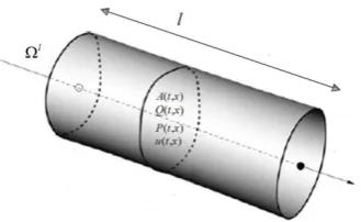
The blood vesselΩl _{can be defined as an elastic tube as shown in the Fig.1, where}_l_{is the length,} _v_{is the volume,} _A₍_{t, x}₎

297

is the cross-sectional area at timet and locationxalong the vessel axis,r(t, x)is radius,u(t, x)is blood velocity, ρ(t, x)is 298

the blood density,η(t, x)is the blood viscosity,Q(t, x)is blood flow andP(t, x)is blood pressure. If the length ofΩl_{is finite}

299

but very small, i.e.l = ∆l, the blood viscosity η∆l_{, velocity}_u∆l _{and density} _ρ∆l _{will be constant, and the cross-sectional}

300

area along the vessel axis will also be constant as A∆l₍_t_{) =} _A∆l₍_{t, x}₎_{, thus}_Ωl _{can then be regarded as the finite but very}

301

small vessel, denoted by Ω∆l_{. In general, blood has been conceptualized as a viscous fluid; therefore, it should follow the}

302

laws of conservation of mass and momentum, which can be described by the basic equations of fluid dynamics: the continuity 303

equation and momentum equation, respectively(? _).

304

1) Continuity equation: The continuity equation for vesselΩl _{can be defined as:}

305

∂A(t)

∂t +

∂Q(t, x)

∂x = 0 (23)

the continuity equation for vesselΩ∆l_{can then be written as:}

306

∆ldA

∆l₍_t₎

dt +Q

∆l₍_{t, x}

(10)

wherexsandxe are the starting and ending locations of vesselΩ∆lrespectively. According to the vessel wall mechanics(?),

307

the blood pressure in Ω∆l _{can be calculated as}

308

P∆l₍_{t, x}_{) =}_P∆l

ext(t, x) +β∆l(

q

A∆l₍_t₎₋q_A∆l

0 ) (25)

whereP∆l

ext(t, x) is the external pressure on the vessel wall, A∆0l is the initial cross-sectional area when there is now blood 309

flow in the vessel, andβ∆l _{is a coefficient which can be defined as:}

310

β∆l₌

√_πh∆l

0 E∆l 0.75A∆l

0

(26)

where h∆l

0 is the thickness of the wall and E∆l is the Young’s modulus( ? ). Integrate Equation(26) along the axis of the 311

blood vessel and differentiate with respect to time. 312

Z xe

xs

∂P∆l₍_{t, x}₎

∂t dx=

Z xe

xs

β∆l

2p

A∆l₍_t₎

∂A∆l₍_t₎

∂t dx. (27)

Some papers show that the section area of artery is changed by only 10% (?? _{), therefor we assume}_A∆l

0 ≈A∆l(t) for the 313

vesselΩ∆l _{, so the average pressure}_P_ˆ∆l₍_t₎_{should satisfy:}

314

dPˆ∆l₍_t₎

dt = β∆l

2p

A∆l

0

dA∆l₍_t₎

dt . (28)

where 315

316

ˆ

P∆l= RXs

Xe P

∆l₍_x₎_dx

∆l (29)

317

Substituting (28) into (24), we can get: 318

2∆lpA∆l

0

β∆l

dPˆ∆l₍_t₎

dt +Q

∆l₍_{t, x}

e)−Q∆l(t, xs) = 0. (30) 2) Momentum equation: The momentum equation for vessel Ωl_{can be written as:}

319

∂Q(t, x)

∂t + ∂ ∂x(

Q(t, x)2

A(t, x) ) +

A(t, x)

ρ(t, x) ·

∂P(t, x)

∂x

+8u(t, x)η(t, x)A(t)

ρ(t, x)r(t)2 = 0.

(31)

For the vesselΩ∆l_{, the above equation can be simplified as}

320 321

ρ∆lZ x

e

xs

∂Q∆l₍_t₎

∂t dx+A

∆l₍_t₎Z x

e

xs

∂P∆l₍_{t, x}₎

∂x dx

+8u

∆l_η∆l_A∆l₍_t₎

(r∆l₍_t₎₎2

Z xe

xs

dx= 0.

(32)

322

AsA∆l

0 ≈A∆l(t), the equation (32) can be simplified as: 323

324

ρ∆l_∆_l

A∆l

0 ·

dQˆ∆l₍_t₎

dt +

8η∆l_∆_l

A∆l

0 (r∆0l)2 ˆ

Q∆l₍_t₎

+P∆l(t, xe)−P∆l(t, xs) = 0.

(33)

325

According to the Zamir’s definitions(?_{) and Equation(30) arterial compliance}_C∆l_{, blood resistance}_R∆l_{of the vessel}_Ω∆l

326

can then be written as: 327

C∆l=d∆V ∆l₍_t₎

dPˆ∆l₍_t₎ =

∆Q∆l₍_t₎_dt

dPˆ∆l₍_t₎ =

Q∆l₍_{t, x}

s)−Q∆l(t, xe)

dPˆ∆l₍_t₎_/dt

=2∆l p

A∆l

0

(11)

328

R∆l₌ 8η∆l∆l

π(r∆l

0 )4 = 8η

∆l_∆_l

A∆l

0 (r∆0l)2

Fluid inertia L∆l _{means the ratio of force difference (include 2 forces: one is the pressure of blood and the other is the}

329

viscous force of blood) and flow rate variation ratio. Therefore,L∆l _is:

330

L∆l=

8η∆l∆l A∆l

0 (r ∆l 0 )2

ˆ

Q∆l₍_t_{) +}_P∆l₍_{t, x}

e)−P∆l(t, xs)

dQˆ∆l₍_t₎_/dt =

ρ∆l_∆_l

A∆l

0

respectively. Therefore, the equations (30) and (33) can be simplified as 331

   

  

C∆ldPˆ∆l(t)

dt +Q

∆l₍_{t, x}

e)−Q∆l(t, xs) = 0

L∆ldQˆ∆l(t)

dt +R

∆l_Q_ˆ∆l₍_t₎₊_P∆l₍_t,x

e)−P∆l(t,xs) = 0.

(34)

APPENDIXB

332

B:HUMANARTERIESNETWORKMODEL

R

₂₅

55

6

Z

sum _ 3

Z

Thoracic aorta I

Thoracic aorta II

Abdominal aorta I

Abdominal aorta II

R. renal

L. renal

Abdominal aorta III

Sup. mensenteric

Abdominal aorta IV

Inf. mesenteric

Abdominal aorta V

Celiac I

Celiac II

Gastric

Hepatic

Splenic

L. vertebral

L. subclavian II

L. radius

L. ulnar I

L. interosseous

L. ulnar II

L. subclavian II

Aortic arch II

Aortic arch I

Ascending aorta

intercoastals

L. com. iliac

L. ext. iliac

L. femoral

L. ant. tibial

L. post. tibial

L. deep femoral

L. int. iliac

R. com. iliac

R. int. iliac

R. ext. iliac

R. deep femoral

R. femoral

R. post. tibial

R. ant. tibial

R. ext. carotid

_{R. int. carotid}

R. carotid

Brachiocephalic

R. subclavian I

R. vertebral

R. subclavian II

R. ulnar I

R. interosseous

R. ulnar II

R. radius

L. int. carotid

L. ext. carotid

(13)

[image:13.595.212.377.86.187.2] [image:13.595.184.417.298.373.2]

Fig. 1: The illustration of the elastic vessel

Fig. 2: The illustration of a segment of large artery

Fig. 3: The large artery model.

[image:13.595.206.391.478.533.2] [image:13.595.205.390.632.694.2]

(14)

[image:14.595.59.541.139.374.2]

Fig. 5: The corresponding electric circuit between left radial artery and ascending aorta. Point B and C are the proximal and distal ends of the radial artery, where the BP can be measured conveniently. Point A is the starting point of central aorta, where the BP is about to estimate.

[image:14.595.191.408.591.653.2]

(15)

(a) (b)

[image:15.595.73.523.202.584.2]

(c) (d)

(16)

(a) RMSE (b) Mean and standard deviation (SD)

[image:16.595.84.504.196.560.2]

(c) correlation coefficient

(17)

[image:17.595.179.415.274.455.2]

Fig. 9: Bland-Altman analysis of central aortic systolic and diastolic blood pressure. The three horizonal lines on each sub-figure indicate: mean+2∗SD, mean, and mean−2∗SD.(a) systolic blood pressure comparison between our proposed method