Sparse Grid Interpolation

Fanzi Meng

A thesis submitted for the degree of

Master of Mathematical Science (Advanced) of

The Australian National University

This thesis is an account of research undertaken between February 2016 and May

2016 at The Department of Mathematics, Faculty of Science, The Australian

Na-tional University, Canberra, Australia.

Except where acknowledged in the customary manner, the material presented in

this thesis is, to the best of my knowledge, original and has not been submitted in whole or part for a degree in any university.

Fanzi. Meng

May, 2016

Foremost, many thanks to my supervisor Stephen Roberts, who has provided

in-valuable feedback and guidance throughout this project.

I am very grateful to Jouke de Baar for inspiring discussions and his warm welcome

and hospitality.

I am pleased to thank all the staff in the Department of Mathematics for all help

that you have provided during my two years of my study at the Australian National

University.

Finally, and most importantly,I would like to express my deepest gratefulness to

my beloved family for all their constant support and patience throughout my study.

Without them, this thesis would have hardly been possible.

For the approximation of multidimensional functions, using classical numerical

dis-cretization schemes such as full grids suffers the curse of dimensionality which is

still a roadblock for the numerical treatment of high-dimensional problems. The

number of basis functions or nodes (grid points) have to be stored and processed

depend exponentially on the number of dimensions, where efficient computation are challenging in the implementation. Recently, the technique of sparse grids has been

introduced to significantly reduce the cost to approximate high-dimensional

func-tions under certain regularity condifunc-tions.

In this thesis, we present the classical sparse grid where the problem is discretized

and solved on a certain sequence of conventional grids with uniform mesh sizes

in each coordinate direction. Furthermore, the different types of sparse grids,i.e.

Clenshaw Curtis sparse grid, have been taken into consideration to compare the

accuracy and complexity of these algorithms. We then describe the sparse grid

combination technique to demonstrate that it is competitive to the classical sparse grid approaches with respect to quality and run time and give proof that the

in-terpolation by using combination approach is the classical sparse grid. We give

details on the basic features of sparse grids and we consider several test problems

up to dimensions. The results of numerical experiments report on the quality of

approximation generated by the sparse grids, and, finally, employ the sparse grid

interpolation for a real-world case to reduce a computationally expensive simulation

model. We aim to obtain an efficient surrogate approximation based on a small

number of simulations.

Declaration iii

Acknowledgements v

Abstract vii

1 Introduction 1

2 Sparse grids 3

2.1 Introduction . . . 3

2.2 Finite element basis functions . . . 3

2.3 One-dimensional multilevel basis . . . 5

2.4 High-dimensional multilevel basis . . . 6

2.5 Sparse grid combination technique . . . 9

2.6 Clenshaw Curtis sparse grids . . . 11

2.7 Proof of combination formula . . . 14

3 Numerical experiments 19 3.1 Sine function . . . 20

3.2 Rosenbrock Function . . . 28

3.3 Gaussian function . . . 35

3.4 Checkerboard . . . 40

4 An experimental study of Hokkaido Nansei-oki tsunami 45 4.1 The Hokkaido-Nansei-Oki tsunami . . . 46

4.2 Results of experiments . . . 46

5 Conclusion 51

Bibliography 53

Chapter 1

Introduction

In numerical analysis, the sparse grid methods are general numerical techniques

for multidimensional integration, interpolation, partial differential equations and

more fields of application. The sparse grid method was evolved due to the curse

of dimension: the exponational dependence of conventional approaches on the

di-mensionality d, a term coined in Bellmann (1961) [1]. The sparse grid method was originally introduced by the Russian mathematician Sergey A. Smolyak in 1963 [2].

Computer algorithms for efficient implementations of such grids were later

devel-oped by Michael Griebel and Christoph Zenger [3]. Compared to full grids O(2nd_), sparse grid method contains only O(2n_·nd−1_{) grid points during the discretization}

process. Under a sufficiently smooth condition, the accuracy of the approximation

to describe a function f is O(h2

nlog(h

−1

n )d

−1_{) with respect to the L}

2 and L∞ norm,

if the solution has bounded second mixed derivatives, in contrast to the full grids

for an accuracy of O(h2_n), in which hn = 2−n represents the mesh size and n is the level of discretization [4]. This way, the curse of dimensionality, is overcome to some

extent. Therefore, the sparse grid needs less points in higher dimensional spaces than conventional full sparse grids to obtain a similar approximation.

In principle, in the sparse grids, we assume that the functions to live in spaces

of functions with bounded mixed derivatives instead. The sparse grid approach

can be genetalized from piecewise linear basis functions to higher-order

polynomi-als. we follow this approach. Starting from an introduction of a one-dimensional

multilevel basis (see Section 2.3), preferably with an H1- and L2- stable one, we

discuss the tensor product approach, based on the 1D multilevel bases such as the

classical piecewise linear hierarchical basis. Then, if we represent a 1D function

as usual as a linear combination of these basis functions, the corresponding coeffi-cients decrease from level to level with a rate which depends on the smoothness of

the function and on the given set of basis functions. From this, a multilevel basis

for the higher-dimensional case (see Section 2.4) is derived from a one-dimensional

multilevel basis by a simple tensor product construction. Here, 1D bases living on

different levels are used in the tensor product construction, the basis functions with

anisotropic support can be obtained in the higher-dimensional case. Now, we check

if the function to be expressed has bounded second mixed derivatives and we could

use a piecewise linear 1D basis function as a starting point, it can be seen that the

corresponding coefficients decrease with a factor proportional to 2−2|l|1 _{where the} multi-index l = (l1,· · · , ld) denotes the different levels involved. Thus, these coeffi-cients whose absolute values are smaller than a prescribed tolerance can be omitted,

we obtain sparse grids [5]. It means that the number of degrees of freedom is needed

for some prescribed accuracy which no longer depends on, up to logarithmic factors,

d exponentially . This allows us to obtain substantially faster solution of moderate-dimensional problems and can enable the solution of higher-moderate-dimensional problems.

As i mentioned before, the sparse grid approach is not restricted to the standard

piecewise linear basis functions. It can be extended to general polynomial degreesp. Also,extensions of the piecewise linear hierarchical basis to interpolates, wavelets or

pre-wavelets have been successfully studied as the univariate ingredient for the tensor

product construction. Finally, the sparse grid is a very widely used approach. The

applications of sparse grids ranges from numerical quadrature, via the discretization

of partial differential equations, to more fields such as data mining.

This thesis will first provide an overview of the principles and features of the sparse grid methods and derive the interpolation properties of the resulting sparse grid

spaces. As a starting point, we use the standard piecewise linear multilevel basis

in one dimension to generate higher dimensions by a tensor product construction.

It is the simplest example of a multilevel series expansion which involves

interpo-lation by piecewise linear. After that, the multilevel polynomial hierarchical bases

can be employed by means of a hierarchical Lagrangian interpolation scheme. We

consider the different types of sparse grids such as Clenshaw Curtis grids to analyze

the quality of approximation. In Chapter 3 we present numerical results of selected

experiments. To show the properties of the sparse grid approximation, we discuss four function examples from two dimensions to higher-dimensions. Furthermore, we

confirm the theoretical proof of the interpolation of sparse grids (in Chapter 2) by

plotting the results of numerical experiments. In Chapter 4, where we apply sparse

grids to the solution of a real-world tsunami problem. We use experimental data to

estimate the uncertain input parameters. We construct a surrogate-based approach

to provide an inexpensive approximation of the output of the computer simulation

for any parameter conguration, which enables us to estimate the parameters without

further solver evaluations. The concluding remarks of Chapter 5 close this discussion

Chapter 2

Sparse grids

2.1

Introduction

In this chapter, we will discuss the problem of interpolating smooth functions with

the help of piecewise d-linear hierarchical bases. Starting from the approximation properties of sparse grids, we study a tensor product-based subspace splitting and an

optimized discretization scheme can be derived. We concentrate on theL2 -and the

L∞norm, and to the respective types of sparse grids. In section 2.2 we introduce the

finite element basis functions exemplied in approximation of functions. Section 2.3

we depict classical one-dimensional sparse grid interpolant, and Sections 2.4 covers the basic concepts and theories in mutlidimensions. In Section 2.5 we introduce the

interpolation by using the combination approach. Section 2.6 describes Clenshaw

Curtis sparse grid. Section 2.7 gives the proof that the combined interpolant is the

hierarchical sparse grid interpolant.

2.2

Finite element basis functions

Let us start with some basic concepts while describing the conventional case of a

piecewise linear finite element basis. The basis functions exemplified in

approxi-mation of functions are in general nonzero on the entire domain Ω. We turn the attention to basis functions that have compact support, meaning that functions are

not zero-valued on only a restricted portion of Ω. We shall restrict the functions to

be piecewise polynomials. This means that the domain is split into subdomains and

the function is a polynomial on each subdomain. At the boundaries between

subdo-mains one normally forces continuity of the function only so that when connecting

two polynomials from two subdomains, the derivative becomes discontinuous.

Let V be a function space spanned by a set of basis functionsψ0,· · · , ψN

V = span{ψ0,· · · , ψN} (2.1)

Given a function f, we wish to approximate f defined by u ∈ V. Let us divide the interval Ω on which f and u are defined into non-overlapping subintervals Ωi_, i= 0,· · · , N

Ω = Ω0∪ · · · ∪ΩN (2.2)

We shall refer to Ωi _{as an element, having numberi. A set of points are introduced} as nodes on each element. Nodes and elements uniquely define a finite element mesh,

which is our discrete representation of the domain in the computations. A common

special case is that of a uniformly partitioned mesh where each element has the same

length and the distance between nodes is constant.

To produce a sufficiently accurate solution we can do refinement, giving a family of nested subspaces V0 ⊂ V1 ⊂, . . .. Elements of Vk are created by the refinement of level k−1 elements.

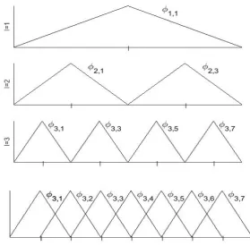
For each spaceVk, two sets of basis functions play important roles in our discussion: the nodal basis ψk

i, i = 0, . . . , Nk (see Fig 2.1, bottom) and the hierarchical basis ϕi, i = 0, . . . , Nk (see Fig 2.1, top). Here, each nodal basis function is a triangle (hat) function of the same extent and the hierarchical basis functions are grouped

into ”levels”, with the functions at the higher levels having a larger extent. We

can convert between the nodal basis representation and the hierarchical basis with

a simple linear matrix transform. The nodal basis ψk_i ∈Vk is defined by

ψ_ik(xj) = δij, δij =

(

1 if i=j;

0 if i6=j. (2.3)

where xj is a node in the mesh with global node number j. On the other hand, the hierarchical basis for Vk is built from that of Vk−1 by adding the nodal basis

functions of Vk associated with the level k nodesxi, i=Nk−1+ 1, . . . , Nk.

The basis function ψi holds two important properties. Firstly, a convenient inter-pretation of coefficients ci as the value of u at node i

u(xi) =

X

j∈Ii

cjψj(xi) =

X

j∈Ii

cjϕj(xi) = ciϕi(xi) = ci. (2.4)

§2.3 One-dimensional multilevel basis 5

Figure 2.1: Piecewise linear hierarchical basis (top) and nodal basis (bottom) of level 3.

2.3

One-dimensional multilevel basis

In the sparse grid approach, a multidimensinal basis on thed-dimensional unit cube based on one-dimensional hierarchical basis is obtained by a tensor product construc-tion. First, we consider a multilevel basis on one-dimensional space and introduce

some notation which is necessary for a detailed discussion of sparse grids for

pur-poses of interpolation or approximation, respectively. Let Ωlbe the equidistant grids

of levell on the interval ¯Ω with mesh sizehl = 2−l. This way the grid Ωl consists of the points

xl,j = j·hl, 0≤j ≤2l (2.5)

Moreover, let Vl be the space of piesewise linear functions on grid Ωl

Vl = span

The basis functions φl,j(x) based on standard hat function having support [xl,j − hl, xl,j+hl]T[0,1] = [(j−1)hl,(j+ 1)hl]T[0,1] are generated as

φl,j(x) = φ

x−j ·h_l

hl = ( 1−

x−j·hl

hl

x∈[(j −1)hl,(j+ 1)hl] T

[0,1]

0 otherwise

This basis is termed nodal basis or lagrange basis. With these function spaces, the

hierarchical increment spaces Wl are defined as

Wl = span{φl,j :j ∈Il} (2.7)

The index set Ii =

j ∈_N, j odd,1≤j ≤2l₋₁

These increment spaces allow us to write Vl as a direct sum of subspaces

Vl =

M

k≤l

Wk (2.8)

The basis corresponding to Wl is just the hierarchical basis of Vl. such that any function u∈Vl can be represented as

u(x) = X k≤l

X

j∈Ii

αk,jφk,j(x) =

X

k≤l ˆ

uk(x), (2.9)

where ˆuk ∈Wk and hierarchical surplus (coefficients)αk,j ∈R.

2.4

High-dimensional multilevel basis

A multidimensional hierarchical basis is obtained from the one-dimensional basis

based on a tensor product construction. Therefore, for a multidimensional basis on

the d-dimensional cube ¯Ω, we define Ωl as anisotropic grid on ¯Ω with equidistant mesh size hlt in each coordinate directiont,t = 1, . . . , d. Here, the l = (l1, . . . , ld)∈

Nd is a multi-index set indicates the level of multi-dimensional sparse grids. The

mesh size is denoted as hl = (hl1, . . . , hld) = 2

−l_{. The grid points x}

l,j of the grid Ωl are considered

xl,j = (xl1,j1, . . . , xld,jd) = j ·hl, 1≤j ≤2

l_{−1 (2.10)}

§2.4 High-dimensional multilevel basis 7

of the tensor product construction.

φl,j(x) = d

Y

t=1

φlt,jt(xt) (2.11)

Now, each of the multidimensional basis functions φl,j that correspond to inner grid points of Ωl with support of the fixed size 2·hl are used to define an associated space Vl

Vl = span

n

φl,j

jt= 0, . . . ,2

lt_{, t= 1, . . . , d}o _{= span}n_φ

l,j : 1≤j ≤2l−1

o

, (2.12)

where this basis

n

φl,j

o

is the standard nodal point basis of the finite dimensional space Vl. Additionally, the hierarchical difference space Wl is obtained by spanning basis functions

Wl = span

n

φl,j :j ∈Bl

o

, (2.13)

with the index set

Bl =

j ∈_Nd _{: 1≤j}

t ≤2lt −1, jt odd, t= 1· · ·d, iflt>0 (2.14)

The hierarchical increments spaces Wl consist of all φi,j ∈Vl, which generate a new sparse gridW_l0, any sparse gridW_lthat meets the order relationW_l< W_l0needs to be constructed before. Therefore, we can define a multilevel subspace decomposition

and the space Vn := Vn can be represented as a direct sum of finite-dimensional subspaces of V

Vn =

M

l1≤n

· · ·M ld≤n

Wl =

M

|l|∞≤n

Wl (2.15)

the limit

lim n→∞V

(∞)

n = _nlim_→∞

M

|l|∞≤n Wl =

∞

[

n=1

V_n(∞) = V (2.16)

where |l|∞ = max1≤t≤dlt. V is simply the underlying Sobolev spaceH01( ¯Ω).

We now define a hierarchical increments space Wl via

Wl = Vl\ d

M

i=1

Vl−ei (2.17)

Again, any function u∈Vn can be uniquely represented by

u(x) = n

X

|l|∞=1

X

j∈Bl

αl,jφl,j(x) =

X

|l|∞≤n ˆ

ul(x), (2.18)

with hierarchical surplus (coefficients) αl,j ∈ R in the hierarchical tensor product basis and ˆul ∈Wl is the hierarchical component functions.

We construct discrete approximation spaces that the same number of invested grid

points leads to a higher order of accuracy. We deal with finite dimensional subspaces

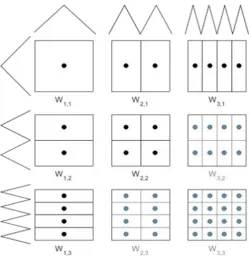
of V with the discrete spaces. First, we summarize some basic properties of the hierarchical subspacesWl according to Bungartz and Griebel (1999) [6]. Concerning the subspaces Wl, we learn the dimension of Wl from (2.13) and (2.14), and the number of degrees of freedom (sparse grid points or basis functions) associated with

Wl:

|Wl| = 2|l−1|1 (2.19)

According to (2.18), the discussion of a subspace contribution to the overall

inter-polant could be based on the maximum norm L∞, the Lp-norm (p = 2 in general) and the energy norm. Now, let us define the Sobolev-space with dominating mixed

derivative H_mix2 . The second mixed derivatives have to be bounded

Dl u = ∂

|l|1_u ∂xl1

1 . . . ∂x

ld

d

, where |l|1 =

d

X

t=1

lt and |l|∞ = max

1≤t≤dlt (2.20)

These functions belong to a Sobolev space

H_mix2 (Ω) := u: Ω→_R:Dl u∈L2(Ω),|l|∞≤2, u|∂Ω = 0 (2.21)

Under this prerequisite, the corresponding coefficients decay rapidly |αl,j| =

O(2−2|l|1_{). It follows that for the components u}

l ∈Wl of u∈H02,mix( ¯Ω) from (2.18) based on L2-norm holds [7].

kulk2 ≤3−d·2−2·|l|1 · |u|H2

mix. (2.22)

That means the elements are bounded and convergent because 3−d_·2−2·|l|1 _{is less} than 1 if u∈H2

mix. It follows the hierarchical basis functions with a small support, and therefore under smoothness assumption, a small contribution to the function

representation, are not included in the discrete space of leveln anymore. Figure 2.2 for the 2D case shows how the supports of the basis functions of the hierarchical

§2.5 Sparse grid combination technique 9

We define the sparse grid function space Vs

n ⊂Vn as

V_ns = M

|l|1≤n

Wl (2.23)

Similar to (2.18), any function u∈Vs

n can be uniquely written as

us_n(x) = n

X

|l|1=1

X

j∈Bl

αl,jφl,j(x) =

X

|l|1≤n ˆ

ul(x) (2.24)

Where ul ∈Wl.

The dimension of the sparse grid space Vs

n (the number of inner grid points in the underlying grid) is given by

|Vs n|=

n−1

X

i=0

2i d−1 +i d−1

!

= (−1)d_{+ 2}n n−1

X

i=0

2i n+d−1 i

!

(−2)d−1−i

= 2n

nd−1

(d−1)! +O(n d−2₎

(2.25)

This, we have

|Vs

n| = O(h

−1

n |log2hn|d−1) (2.26) For the interpolation error of a function f ∈H2

mix in the sparse grid space Vns gives

||f −us_n||2 = O(h2nlog(h

−1

n )

d−1_{) (2.27)}

For more details and proof, we can find here Garcke (2004).

2.5

Sparse grid combination technique

A sparse grid solution obtained by a combination of anisotropic full grid solutions is

often the so-called combination technique [8]. The combination technique is a

multi-variate extrapolation type method to achieve a function representation on a sparse grid. It exploits the approximation properties of sparse grids mentioned beforehand:

the discretization of the function applies to a nodal discretization. For the solution

of partial differential equations, the equations are decoupled into smaller systems on

the grids and are linearly combined. Furthermore, the finite element discretization

Figure 2.2: In two-dimensional space, the sparse grid space Vs

3 contains the upper triangle of

spaces shown in black.

preserved. The advantages of the combination technique over working directly in

the hierarchical basis are that the matrix graph has considerably fewer connections

and the resulting linear systems are sparse, in contrast, the stiffness matrices of

sparse finite elements are not sparse and computations of the matrix-vector-product

come with a high cost [9].

For the discretisation of the function space V we use a generalisation of the sparse grid combination technique. We restrict to a bounded domain Ω = [a, b]d _and

consider a certain sequence of anisotropic grids Ωl = Ωl1,...,ld which have different

but uniform mesh sizes in each coordinate direction with ht= 2−lt, t= 1, . . . , d. In the original combination technique considers all grids Ωl with indices

|l| = l1 +· · ·+ld = n+ (d−1)−q, q = 0, . . . , d−1, lt >0 (2.28)

A finite element discretisation using piecewise d-linear functions

φl,j(x) = d

Y

t=1

φlt,jt(xt) (2.29)

§2.6 Clenshaw Curtis sparse grids 11

the discrete function space Vl = span

n

φl,j, jt= 0, . . . ,2lt, t= 1, . . . , d

o

on grid Ωl.

A function ul ∈Vl is represented as

ul(x) =

2l1

X

j1=0 · · ·

2ld

X

jd=0

αl,jφl,j(x), (2.30)

and uses combination coefficients to add up the partial solutions ul from each grid combined to obtain the solution uc

n on the corresponding sparse grid according to the combination formula

uc_n(x) = d−1

X

j=0

(−1)j d−1 j

!

X

|l|=n−j

ul(x). (2.31)

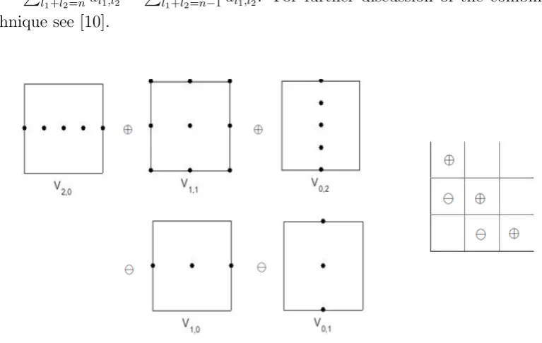
The combination technique constructs a grid function uc

n on a sparse grid space V_ns, see Fig 2.3. For examples, in two dimensional space, it clearly shows that uc_n = P

l1+l2=nul1,l2 −

P

l1+l2=n−1ul1,l2. For further discussion of the combination technique see [10].

Figure 2.3: Combination technique with sparse grid level 2 in two dimension.

2.6

Clenshaw Curtis sparse grids

As we have seen, it is the hierarchical finite elements (Peano 1976) and the

hierar-chical bases (Yserentant 1986) to a tensor product construction with its underlying

hierarchical subspace splitting that the Zenger’s sparse grid concept (Zenger 1991)

closely related technique had been studied for purposes of approximation, or

numeri-cal integration of smooth functions. The Russian literature that has to be mentioned

here is those of Smolyak (1963) studied classes of quadrature formulas of the type

U_n(d)f = n

X

i=0

(U_i(1)−U_i(1)₋₁)⊗U_n(d₋−_i1)

!

f (2.32)

where Un(d) denotes a d-dimensional quadrature formula based on the 1D rule Un(1) with a tensor product. Functions suitable for the Smolyak approach typically live

in spaces of bounded (Lp-integrable) mixed derivatives which are closely related to

our choice of uin (2.20).

For a detailed discussion of those methods, we consider a quadrature known as

Clenshaw Curtis quadrature. The use of Clenshaw Curtis quadrature rule forms a

sparse grid. The rules provided an indexed family have a nested set, so that all

the abscissas from one rule are included in the next. The values of the abscissas and weights can be easily computed. The construction of a nested family requires

that the order of the rules in the indexed family grows exponentially. We define

the Clenshaw Curtis formula, denoted byCCn as the interpolatory quadrature rule constructed on the Chebychev nodes [11].

Suppose a sparse grid constructed for a D-dimensional quadrature of function f. We consider an indexed family of underlying 1D factor quadrature rules over the

interval [0,1]. The interpolating polynomial that we integrate can be expressed in a

compact form as:

I(1)(f) =

Z Γ1 f(x)dx' N X n=0

f(xn)wn (2.33)

This is an (N + 1) points (nodes) quadrature rule having (N + 1) real values wn called weights expressing the integral I(1) _{as a weighted sum of samples of f.}

The trapezoid rule, we write the approximation of integral above as:

U_l(1)f = Nl

X

n=0

f(xn,l)wn,l = 1 2hl

f(0) +f(1) + 2 Nl−1

X

n=1

f(xn,l)

!

(2.34)

where hl = ₂l1−1, Nl= 2l−1 + 1, xn,l =nhl= ₂ln−1, wn,l =

h

1 2hl,

1

hl,· · · ,

1 2hl,

1

hl

i

In a Clenshaw-Curtis quadrature rule, Chebychev nodes for a given natural number

Nl are: xn,l = 1₂

1−cosπ_N(n−1)

l−1

, n= 1,· · ·, Nl.

§2.6 Clenshaw Curtis sparse grids 13

endpoints, and then by rules which successively add points between each pair of

points in the preceding rule [12].

A multidimensional quadrature rule is formed by the product of underlying 1D rules.

Let U_l(1)

i :V →R and f : Ω

d _→

R. It can be written as:

U_lDf(x) =U_l(1)

1 ⊗ · · · ⊗U

(1)

ld

f(x1,· · · , xd)

=U_l(1)

1 ⊗ · · · ⊗U

(1)

ld−1





N_ld

X

nd=1

f(x1,· · · , xd,nd)





=U_l(1)

1 ⊗ · · · ⊗U

(1)

ld−2





N_ld

X

nd=1

U_l(1)

d−1f(x1,· · · , xd,nd)wld,nd





=U_l(1)

1 ⊗ · · · ⊗U

(1)

ld−2 N_ld−1

X

nd−1=1 N_ld

X

nd=1

f(x1,· · · , xd−1,nd−1, xd,nd)

· · ·

=U_l(1) 1





Nl₂

X

n2=1 · · ·

N_ld

X

nd=1

f(x1· · ·xd,nd)wl3,n3· · ·wld,nd





= Nl₂

X

n2=1 · · ·

N_ld

X

nd=1

U_l(1)

1 f(x1· · ·xd,nd)wl2,n2· · ·wld,nd

= Nl1

X

n1=1 · · ·

N_ld

X

nd=1

f(x1,n1· · ·xd,nd)wl1,n1· · ·wld,nd

(2.35)

where N =Qd

i=1Nli.

This productQ

is a monic polynomial of degree D. The interpolation error satisfies

|ID_{f −U}D_{f| = O(N}−m/d

l ) (2.36)

For function f in the space

W_mixm,∞([0,1]d) =

(

f : [0,1]d→_R; max

|l|≤mk

∂|l|_f

∂xl1

1 . . . ∂x

ld

d

k∞≤ ∞

)

(2.37)

where d is the dimensions and m is the bounded value. The 1-D nodal points are Θ(1)_l ={xl,1,· · · , xl,d}. The sparse grid nodal set is:

Θ(_lD) = [

|l|≤l+d−1

Θ(1)_l

1 × · · · ×Θ

(1)

We define the difference relations as ∆(1)_l f =U_l(1)−U_l(1)₋₁f. Thus, the sparse grid multidimensional quadrature rule can be expressed as:

U_l(D)f = X

|l|≤l+d−1

∆(1)_l

1 ⊗ · · · ⊗∆

(1)

ld

f (2.39)

We say that this product rule has a product level of |l| = P

i≤Dli, where l = (l1,· · · , ld)∈Nd is a multi-index.

A sparse grid can be indexed by the sparse grid level l that uses weighted combina-tions of those product rules. The lowest sparse grid level is taken to be 0. So the

sparse grid of sparse grid level 0 is equal to the product rule of product level 0. To construct the sparse grid in a Clenshaw-Curtis quadrature rule, we have:

A(l, D) = X

l−D+1≤|i|≤l

(−1)l−|i| D−1

l− |i|

!

U_l(1)

1 ⊗ · · · ⊗U

(1)

ld

(2.40)

Formally, to describe a sparse grid using the Clenshaw Curtis rule is to substitute

CCli for each generic quadrature rule Uli. Consider the specific formulas for sparse

grid level one in dimension two which are products of the 1D Clenshaw Curtis rules:

A(1,2) =CC1⊗CC0

+CC0⊗CC1

−CC0⊗CC0

(2.41)

2.7

Proof of combination formula

We discuss the relationship of hierarchical sparse grid interpolation and interpolation

by using combination technique. It is shown that the combined interpolation is

iden-tical with the hierarchical sparse grid interpolation (J Garcke, 2012). The proof can

be seen by rewriting each ul in their hierarchical representation and some straight-forward calculation using the telescoping sum. Moreover, the proof is extended

from two and three dimensions to the high-dimensional cases. To demonstrate the

advantages of the combination technique over working directly in the hierarchical basis, we consider certain equation problems with numerical experiments (Chapter

3). The outputs of numerical implementation are provided to compare these two

interpolations and estimate computational accuracy.

For a given function uthe interpolant uc

n using the combination technique (2.31) is the hierarchical sparse grid interpolant us

§2.7 Proof of combination formula 15

Proof. We start in a two dimensional case. We can have

us_n= X k1+k2≤n

ˆ uk1,k2

and according to the combination formula, we write

uc_n= X

|l|=n ul−

X

|l|=n−1

ul

We learned in the equations (2.9) and (2.24), we can rewrite the function ul in two dimensional space as

ul(x) =

X

|k|≤l

X

j∈Bk

αk,jφk,j(x) =

X

|k|≤l ˆ uk1,k2

Therefore, following the equation, we now define

X

|l|=n ul=

X

|l|=n

X

|k|≤l ˆ

uk1,k2, and

X

|l|=n−1

ul =

X

|l|=n−1

X

|k|≤l ˆ uk1,k2

For the combined interpolant we get as in

uc_n = X

|l|=n

X

|k|≤l ˆ uk1,k2 −

X

|l|=n−1

X

|k|≤l ˆ uk1,k2

= X

l1+l2=n

X

k1≤l1

X

k2≤l2 ˆ uk1,k2 −

X

l1+l2=n−1

X

k1≤l1

X

k2≤l2 ˆ uk1,k2

=X

l1≤n

X

k1≤l1

X

k2≤n−l1 ˆ uk1,k2 −

X

l1≤n−1

X

k1≤l1

X

k2≤n−l1−1 ˆ uk1,k2

=X

l1=n

X

k1≤l1

X

k2=0 ˆ uk1,k2 +

X

l1≤n−1

X

k1≤l1

X

k2≤n−l1 ˆ uk1,k2 −

X

k2≤n−l1−1 ˆ uk1,k2

!

=X

l1=n

X

k1≤l1

X

k2=0 ˆ uk1,k2 +

X

l1≤n−1

X

k1≤l1

X

k2=n−l1 ˆ uk1,k2

=X

l1≤n

X

k1≤l1

X

k2=n−l1 ˆ uk1,k2

= X

k1≤n−k2

X

k2≤n ˆ uk1,k2

= X

k1+k2≤n ˆ uk1,k2

(2.42)

where ˆuk = ˆuk1,k2 = ˆuk1,k\k1 = ˆuk1,k2 [13]. Thus, the expression of interpolant using combination technique uc

n is exactly the same as the hierarchical sparse grid interpolant us

for higher dimensional spaces in terms of the statement (2.42), known as the base

case. By the principle of induction, the lemma is true in any dimensions. Recall the

combination technique formula

uc_n(x) = d−1

X

k=0

(−1)k d−1 k

!

X

|l|=n−k ul(x)

We note that the coefficients (the numbers in front of each ulterm) follow a pattern

d= 2: 1 -1

d= 3: 1 -2 1

d= 4: 1 -3 3 -1

d= 5: 1 -4 6 -4 1

d= 6: 1 -5 10 -10 5 -1

This sequence is known as Pascal’s triangle. Each of the numbers is found by

adding together the two absolute numbers directly above it and put minus sign if

the number k is odd.

Thus, the combination function uc

n whend=n can be expressed by the function at d =n−1. Any combination technique functions can be rewritten as two standard terms with respected to the previous function. Then, according to the principle of

induction, we prove uc_n = us_n is true for d = n. We get the general form by using

Zd−→Zd−1|l1, . . . , ld−→l2, . . . , ld in the following way

uc_n = d−1

X

k=0

(−1)k d−1 k

!

X

|l|=n−k ul

=





d−2

X

k=0

(−1)k d−2 k

! X

|l|=n−k ul



−





d−2

X

k=0

(−1)k d−2 k

! X

|l|=n−k−1

ul   =  

d−2

X

k=0

(−1)k d−2 k

!

X

|l|=n−k

X

|k|≤l ˆ uk  −  

d−2

X

k=0

(−1)k d−2 k

!

X

|l|=n−k−1

X

|k|≤l ˆ uk





§2.7 Proof of combination formula 17

=





d−2

X

k=0

(−1)k d−2 k

! _n

X

l1=0

X

|l2|≤n−k−l1

X

|k|≤l ˆ uk   −  

d−2

X

k=0

(−1)k d−2 k

!_n−1 X

l1=0

X

|l2|≤n−k−l1−1

X

|k|≤l ˆ uk





= n−1

X

l1=0

X

k1≤l1





d−2

X

k=0

(−1)k d−2 k

!

X

|l2|≤n−k−l1

X

|k|≤l ˆ uk−

d−2

X

k=0

(−1)k d−2 k

!

X

|l2|≤n−k−l1−1

X

|k|≤l ˆ uk





+X

l1=n

X

|l2|=0 ˆ

uk (Where ul= ˆul = 0 if any ifli <0, l= (l1,· · · , ld))

= n−1

X

l1=0

X

k1≤l1

X

k2+···+kd≤n−l1 ˆ uk1,k2 −

X

k2+···+kd≤n−l1−1 ˆ uk1,k2

!

+X

l1=n

X

k1≤l1

X

k2+···+kd=0

ˆ uk1,k2

(obtained from induction hypothesis)

= n−1

X

l1=0

X

k1≤l1

X

k2+···+kd=n−l1 ˆ uk1,k2 +

X

l1=n

X

k1≤l1

X

k2+···+kd=0

ˆ uk1,k2

= n

X

l1=0

X

k1≤l1

X

k2+···+kd=n−l1 ˆ uk1,k2

= X

k2+···+kd≤n

X

k1≤n−k2−···−kd

ˆ uk

= X

k1+···+kd≤n

ˆ uk

Chapter 3

Numerical experiments

In the preceding section, we theoretically proved that the combined interpolant is

identical with the hierarchical sparse grid interpolant. However, to demonstrate the

equivalency of these two interpolants and identify properties and patterns, the way is to make numerical experiments. In this section, we report a collection of numerical

results and estimate the quality of the approximations for different problems solved

on the hierarchical sparse grids and the combination approach. We start with the

discussion of the basic interpolation properties of sparse grid methods applied to a

simpler 2D model problem. Then we turn to the approximation of the Rosenbrock

function, Gaussian equation and Checkboard on sparse grids in higher

dimension-ality. For measuring the error, we consider the errors discrete maximum norm and

the discrete L2-norm on grids. In low dimensionalities, we can compute the error

terms numerically. In higher dimensionalities we can still approximate the error

stochastically with Monte Carlo or quasi-Monte Carlo methods. Since the curse of a fixed grid in D dimensions requires ND _{points where are too difficult to} imple-ment, the Monte Carlo method is both interesting and useful for error estimation of

a higher dimensionality. Monte Carlo methods are usually presented as estimates

of averages which in turn are integrals, _N1 PN i=1

|f(Xi)−u(Xi)|2

u(Xi) ≈

R

|f(Xi)−u(Xi)|2. The error typically decreases proportionally to √1

N. In the context of solvers, it is important that the influence of the sparse grid level on the accuracy of the

inter-polants. Thus, we attempt to find out a suitable level in which we can obtain a high

quality approximation and estimate the rate of convergence of prediction errors for

an increasing sparse grid level. Moreover, Let us now visualize the sparse grid. Our model problems cover the classical sparse grids and the type of Clenshaw-Curtis

grids. We compare the accuracy of the approximations of these two types of sparse

grids and investigate the efficiency of the performance. For our numerical tests we

used the MATLAB implementation of sparse grid package done in the hierarchical

subspaces can be found here [14]

In the following we will consider the following four functions:

f(x, y) = sin(10x) + sin(10y), (3.1)

with the domain [0,1]2.

f(xi) = d−1

X

i=1

100×(xi+1−x2i)

2

+ (xi −1)2

, (3.2)

with the domain [−2,2]d.

f(xi) = exp − d

X

i=1

xi−µ 2σ2

!

, (3.3)

with the domain [0,1]d_.

A discontinues function with a 2×2 checkerboard pattern with the domain [0,1]2

f(xi) =







exp−Pd i=1

xi−µ

2σ2

, if xi ∈[0,0.5]2, or xi ∈[0.5,1]2;

−exp−Pd

i=1

xi−µ

2σ2

, otherwise. (3.4)

3.1

Sine function

The first test function is a low dimensional Sine function, defined on the unit

hy-percube [0,1]2. It is a simple and well-defined function.

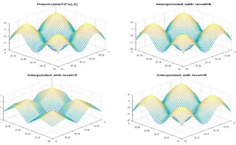
Figure 3.1: The exact solution and the hierarchical sparse grids interpolantusn (on the top).The

combined interpolantuc

§3.1 Sine function 21

Fig 3.1 shows the approximations of the exact solution of (3.1) generated by

the hierarchical sparse grid interpolant and combined interpolant. We study the

accuracy of the hierarchical Lagrangian approach for the classical sparse grids and

combination approach. For the same grid level 6, the hierarchical sparse grids

inter-polant (the upper-right corner) is equivalent to the interinter-polant by using combination

approach (the lower-right corner). Moreover, Fig 3.1 visually illustrates the effect of

the choice of sparse grid levels that the combined interpolant with level = 2 gener-ates a lower accurate and rough approximation than the combined interpolant with

level = 6. A higher accurate approximation can be obtained based on the sparse grid depth (level).

Figure 3.2: The contour plots of exact solution (in the upper-left coner) and the hierarchical sparse grids interpolant (in the upper-right coner); In the second row, the contour plots of the combined interpolants with level=2 and level=6, respectively.

In Fig 3.2, the sparse grid points visualized on the contour plots of the

inter-polants, we see that is the classical uniform sparse grid. For two dimensional case,

Figure 3.3: The contour plots of Clenshaw Curtis sparse grids interpolant with level=2 (the left hand side) and of Clenshaw Curtis sparse grids interpolant with level=6 (the right hand side).

of grid points compared with the classical grid, but it constructed on the Chebychev nodes, see Fig 3.3. Fig 3.4 and Fig 3.6 show the absolute error of the solution us n that was computed on the hierarchical sparse grid and the error that was obtained

by the combination approach uc

n. As expected, the error on the hierarchical sparse grid and on the combined grids have the same behaviour and size. In contrast to

that, the absolute error of combined solution with level = 2 shows large errors, see Fig 3.5. The comparison of interpolation error for level = 6 of classical and Clenshaw Curtis sparse grid choice (see Fig 3.4 and Fig 3.7) demonstrates that the

approximation generated by Clenshaw Curtis grid are more accurate than that of

the classical grid. As we can see, the Clenshaw Curtis process reduces the error equally over the whole domain. With a few terms, these are pretty accurate over

the normal range that they are calculated. However, with a finite number of terms

the sine function is never exactly equal to a polynomial.

In Fig 3.8, the convergence behaviour with respect to the RMSE error of the given

function and for level l ∈ {0,· · · ,6} is provided. In addition to the error plots, we show the curves of expected sparse grid convergence (reference) due to the

in-terpolation accuracy (2.27). Since the prediction error goes extremely small and

the number of grid points grows exponentially as the sparse grid level increases, we

§3.1 Sine function 23

Figure 3.4: Absolute error for the hierarchical sparse grids interpolant with level=6.

Figure 3.5: Absolute error for the combined interpolant with level=2.

Figure 3.7: Absolute error for Clenshaw Curtis sparse grid with level=6

Figure 3.8: Convergence of the RMSE error of the function against an increasing level of grids. The numerically observed rate of convergence for two interpolants , compared to a reference line.

Level Points Max.Abs.Error Rel.Error

1 5 3.4494 1.7880

2 13 1.3047 0.4765

3 29 0.3634 0.1377

4 65 0.0965 0.0356

5 145 0.0239 0.0089

6 321 0.0061 0.0023

Table 3.1: The maximum absolute error and relative error for the hierarchical sparse grid interpolant

From the Fig 3.8, we determine the hierarchical sparse grid and sparse grid

combination technique generate the same relative prediction errors at each level

§3.1 Sine function 25

Figure 3.9: Convergence of the RMSE error of the function against an increasing level of grids. The numerically observed rate of convergence for two interpolants.

straight line for an increasing grid level. Compared with the theoretical error analysis

O(h2

nlog(h

−1

n )d

−1_{), the plot of convergence runs roughly parallel to the reference line.}

The rate of convergence is around -1.8. The table 3.1 displays that the maximum

absolute errors and the relative errors are decreasing with a constant rate as the

number of grid points increases.

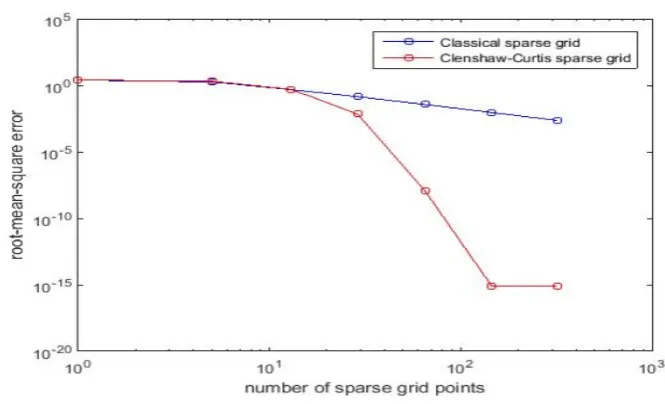
Next, we turn to Clenshaw Curtis sparse grid. In Fig 3.9, we see that the RMSE

error for Clenshaw Curtis grid decreases dramatically against an increasing level of grids. It fast converges to 10e−15 _{at grid level 5, and then be a constant. As}

we expect, the polynomials are never completely accurate. Fig 3.10 illustrates the

cost for computing the interpolants. The combined sparse grid interpolant can be

obtained at a small cost in lower grid levels, but the curves of cost of combined

grid intersects the curves of cost of hierarchical grids and Clenshaw Curtis grids at

sparse grid level 8 and level 9, respectively. Due to the more sophisticated algorithms

required in the polynomial case, the additional cost of computing the interpolant of

Clenshaw Curtis grid is considerably higher compared to the classical sparse grid

interpolation of function values. However, as the grid level increases, the rate of cost decreases, as fewer function evaluation will require a computation. Thus, the

performance is competitive. With these results supporting the efficiency of mesh

refinement on sparse grids and the combination technique approximation, we close

Figure 3.10: Time to compute 1000 values with these three types of sparse grids.

Figure 3.11: Convergence of the RMSE error of the multi-dimensional functions against an increasing level of grids on the classical grid.

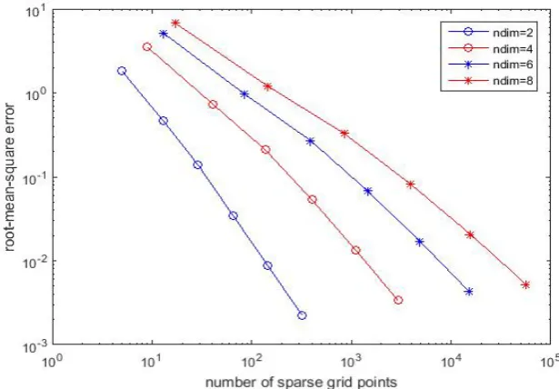
In Fig 3.11, we present a summary of the convergence behaviour with respect to multi-dimensions (d ∈ {2,4,· · · ,8}). We can clearly see that it has a fast con-vergence rate even for a higher dimensional case. Similarly, Fig 3.20 illustrates that

the RMSE error for Clenshaw Curtis grid rapidly decreases down to 10e−15 _{for all}

dimensions, and then it keeps constant as grid level increases. We compare the

§3.1 Sine function 27

3.13 and Fig 3.14. the computational cost increases exponentially with the number

of dimensions. The computational cost of the Clenshaw Curtis grid interpolation is

sightly higher than that of the uniform sparse grid interpolation.

Figure 3.12: Convergence of the RMSE error of the multi-dimensional functions against an increasing level of grids on the Clenshaw Curtis grid.

Figure 3.14: Time to compute 1000 values with these three types of sparse grids.

3.2

Rosenbrock Function

As the second test function, we consider the multi-dimensional Rosenbrock function,

which is often used as a performance test problem for optimization algorithms. The

Rosenbrock function, also referred to as the Valley or Banana function. The function

is unimodal, and the global minimum (f(x) = 0, atx= (1,· · ·,1)) lies in a narrow, parabolic valley. However, even though this valley is easy to find, convergence to the

minimum is difficult (Picheny et al., 2012) [15]. We use the following rescaled form

of the Rosenbrock function (3.2) on the domain[0,1]d_{. Fig 3.11 is an illustration of}

the two-dimensional case.

g(xi) = f(4xi −2) (3.5)

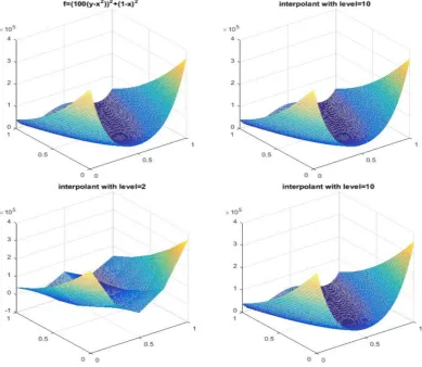
Fig 3.15 shows that the approximations of the exact solution generated by the

hierarchical sparse grid interpolant and combined interpolant. Again, the effects of

the improved sparse grid levels of our interpolation are evident. It also illustrates

that the hierarchical sparse grids interpolant (the upper-right corner) is identical

to the interpolant by using combination approach (the lower-right corner). In Fig 3.16, the sparse grid visualized on the contour plots of the interpolants, we see that

the used sparse grid is of the type classical sparse grid and the Clenshaw-Curtis.

It can be shown that the interpolation of Clenshaw-Curtis grids with level = 2 has obtained relatively accurate approximation of the exact solution compared to

§3.2 Rosenbrock Function 29

two-dimensional case, the sparse grids consist of 13 points with level = 2 is, and of level = 10 is 7169 points, respectively.

Figure 3.15: The exact solution and the hierarchical sparse grids interpolantus

n(on the top).The

combined interpolantuc_nwith level 2 and 10 ( on the bottom).

In Fig 3.17 and Fig 3.18, we present the absolute errors resulting from the

hier-archical sparse grids and the combination approach. Obviously, the errors are the

same, which confirms the theoretical proof in section 2.7. Fig 3.19 shows that the

relative errors on the hierarchical sparse grids are large near the global minimum

which is inside a long, narrow and parabolic shaped flat valley. It does make sense in

terms of the relative error formula (Rel = |measuredvalue_truevalue−₊₁truevalue|). Since the relative error formula has the minimum value as a denominator, we add a small value such as 1 on the denominator. To get an impression of the Clenshaw-Curtis process, Fig

3.20 and Fig 3.21 show the absolute error and the relative error with girdlevel = 10, respectively. We can see the error is extremely small and the Clenshaw-Curtis

pro-cess reduces the absolute error equally over the whole domain. For the same reason,

§3.2 Rosenbrock Function 31

Figure 3.17: Absolute error for the hierarchical sparse grids interpolant with level=10.

Figure 3.18: Absolute error for the combined interpolant with level=10

Figure 3.20: Absolute error for the Clenshaw-Curtis grids interpolant with level=10.

Figure 3.21: Relative error for the Clenshaw-Curtis grids interpolant with level=10.

Fig 3.22 shows the relative prediction error for 2D example for an increasing

number of grid levels. From Fig 3.22, we determine the hierarchical sparse grid and

sparse grid combination technique generate the same relative prediction errors for

all grid levels. The solid line, the expected sparse grid convergence, indicates the

behaviour of the error of sparse grids with respect to the problem of interpolating

a given function. We observe an almost straight line roughly parallels to the solid

line for an increasing grid level. The rate of convergence is around -1.7. In Fig 3.23, a summary of the convergence behaviour with respect to multi-dimensions

(d ∈ {2,4,· · · ,10}) is provided. For all dimensions presented, we can see that the convergence rate is decreasing as the dimension increases. A strong support of

our proof in section 2.7 indicates the interpolant using the combination technique

Clenshaw-§3.2 Rosenbrock Function 33

Curtis grids. Fig 3.24 illustrates that the RMSE error for Clenshaw Curtis grid

rapidly decreases down to 10e−10 _{from grid level 1 to level 2, and then it keeps}

constant as grid level increases. The achieved accuracy will be compared to the

results of interpolation on the classical sparse grids. With the Clenshaw Curtis

process advancing, the higher accurate approximation of exact solution comes to

fruition. Finally, to get an efficiency of the sparse grids process, Fig 3.25 and Fig

3.26 show the computational cost for the classical grid and the Clenshaw Curtis

grid. The Clenshaw-Curtis sparse grid interpolant can be obtained at a very small

additional cost compared to the classical sparse grid interpolant of function.

Figure 3.22: Convergence of the RMSE error of the function against an increasing level of grids. The numerically observed rate of convergence for two interpolants, compared to a reference line.

Figure 3.24: Convergence of the RMSE error of the multi-dimensional functions against an increasing level of grids. The numerically observed rate of convergence for two interpolants.

Figure 3.25: Time to compute 1000 values with the Classical sparse grids for multidimensions.

§3.3 Gaussian function 35

3.3

Gaussian function

All examples have so for been treated with the classical sparse grid, the Clenshaw

Curtis grid and the combination approach, we want to present one more result for

a Gaussian function. On Ω = [0,1]d_{, let}

f(xi) = exp − d

X

i=1

xi−µ 2σ2

!

, (3.6)

where µand σ are constants.

Figure 3.27: The exact solution (on the top).The hierarchical sparse grids interpolant us n and

Figure 3.28: The contour plots of exact solution (in the upper-left corner) and the combined interpolants (in the upper-right corner); In the middle, the contour plots of the hierarchical sparse grids interpolant with level=2 and level=7, respectively; on the bottom, the contour plots of Clenshaw-Curtis grids.

Fig 3.27 shows the true value and the approximation of a Gaussian function in

2D. It should come as no surprise that the approximation generated by the

hierar-chical sparse grids interpolant is the same as the interpolant by using combination

technique. The improved the sparse grid levels (depth) have effects on the quality of approximations. Fig 3.28 shows the classical sparse grid and the type of Clenshaw

Curtis grids with 13 grid points (l = 2, left), and 705 grid points (l = 7, right). In

Fig 3.29 and Fig 3.30, we compare the error on the classical sparse grid and on the

combination approach. Fig 3.29 and Fig 3.30 show a gain in accuracy with higher

§3.3 Gaussian function 37

the contour plots of errors, the different types of grid nodes influence the pattern of

resulting errors. The classical sparse grids show large errors in the middle, in

con-trast with that, the Clenshaw Curtis grids generate large error around the corners.

Figure 3.29: Absolute error for the hierarchical sparse grids interpolant with level=2 and level=7, respectively.

Figure 3.31: Convergence of the RMSE error of the function against an increasing level of grids. The numerically observed rate of convergence for two interpolants, compared to a reference line.

Figure 3.32: Convergence of the RMSE error of the multi-dimensional functions against an increasing level of grids. The numerically observed rate of convergence for two interpolants.

In Fig 3.31, we present the convergence of the conventional sparse grid method

with the curves of expected sparse grid convergence (reference). We observe that

the rate of convergence decreases against the number of sparse grid points. The

curves of the classical sparse grid convergence is not parallel to the reference line,

but it reasonably works well in 2D. The rate of convergence is around -1.5. Fig

3.32 illustrates the convergence behaviour on the classical sparse grid for higher dimensions. For higher dimensional case, it suggests slow convergence, convergence

in the L2 norm is not achieved in regions. It seems that the convergence behaviour

needs large number of grids points to appear. This was to be expected, since this

is consequence of the fact that Gaussian function distribution mostly sits in a thin

§3.3 Gaussian function 39

convergence behaviour on the Clenshaw Curtis sparse grid for higher dimensions.

Again, as in our previous experimental results of the classical grids, we can see

that the sparse grid method achieves a fast convergence rate in 2D but it does not

work well for high-dimensional cases. Compared to the classical sparse grid, the

Clenshaw Curtis has lower rate of convergence in the higher dimensions. We check

if the sparse grids provide a good compromise between accuracy and computational

cost. Fig 3.34 and Fig 3.35 indicate that the computational cost of Clenshaw Curtis

grid is considerably higher compared to the classical sparse grids interpolation of

function.

Figure 3.33: Convergence of the RMSE error of the multi-dimensional functions against an increasing level of grids. The numerically observed rate of convergence for two interpolants.

Figure 3.35: Time to compute 1000 values with the Clenshaw Curtis sparse grids for multidi-mensions.

3.4

Checkerboard

The last example of this section demonstrates that our approach is limited to

dis-continuous function such as the Checkerboard, since for the conventional sparse

grid methods, a priori selection of grid points, optimal under certain smoothness

conditions. Unfortunately, the discontinuous function itself cannot be successfully

approximated by a continuous sparse grid interpolant in the first place.

We first consider two dimensional problems in Ω = [0,1]2_{. The class labels±1 have}

been assigned in a 2 ×2 and 3×3 checkerboard pattern. A 2 ×2 checkerboard

pattern is provided, see Fig 3.36. Now, looking at two dimensional the discontinues

function with a checkerboard pattern

f(xi) =







exp−Pd

i=1

xi−µ

2σ2

, if xi ∈[0,0.5]2, or xi ∈[0.5,1]2;

−exp−Pd

i=1

xi−µ

2σ2

, otherwise. (3.7)

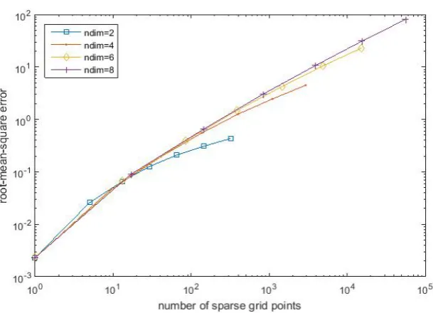
In Fig 3.37, we show the convergence behaviour with respect to L2 error for

regular sparse grids. In addition to the error plots, we present the curves of expected

sparse grid convergence (reference). Moreover, Table 3.2 provides the numerical

values of maximum errors and relative errors on conventional sparse grid methods.

Due to the violation of the smoothness requirements, the L2 error converges much

worse thanO(h2_nlog(h−_n1)d−1) as in the smooth case. As we can see for this measure, using more grid points does not necessarily lead to a better accuracy, the error can

increase. Investigating the accuracy if depending on how the separation manifold is located relative to the sparse grid structure, we examine a 3×3 checkerboard pattern. Fig 3.38 indicates that again low convergence rates are encountered. We cannot

§3.4 Checkerboard 41

Figure 3.36: The class labels -1 (red) and +1 (blue) have been assigned in a 2×2 checkerboard pattern.

Figure 3.38: Numerically observed convergence of the RMSE error of the 3×3 checkerboard function against an increasing level of grids.

Finally, and to give a checkerboard that a similar behaviour can be expected in

higher-dimensional settings, we show the error for a checkerboard in 3D case, see

Fig 3.35. We have shown that the effect that checkerboard functions violate the

sparse grids’ smoothness requirements, non-continuous functions have been studied.

Whereas the classical refinement criterion does not target the error, some refinement strategies can further improve the convergence of the error quite significantly. For a

detailed discussion of an extension of the classical sparse grid approach by spatially

§3.4 Checkerboard 43

Chapter 4

An experimental study of

Hokkaido Nansei-oki tsunami

In this chapter, we look for a surrogate method to provide an approximation of the

output of an input-output relationships using as few model evaluations as possible.

Many engineering design problems involve black-box functions whose values are

outcomes of computationally expensive simulations, so an approximation model of

the outcome is used instead. For example, an input-output system with a known

multivariate input distribution p(x), the Monte Carlo statistical sampling allows us to estimate the statistical moments of the output u(x). However, Monte-Carlo approaches of exploring the input parameter space require a large number of L of expensive simulations. One approach of alleviating the burden is by developing

surrogate models, alternatively known as response surface models, metamodels or emulators (Sacks at al., 1989) [16]. The surrogate approximation is based on a small

set of M L simulations, known as ’samples’ or ’training data’. Our objective is to build an accurate and efficient surrogate approximation by using a small set of

M samples. Moreover, since we increase the number of uncertain input parameters, such studies suffer from the curse of dimensionality. In this work, we use the sparse

grid interpolation to reduce the curse of dimensionality. A sparse adaptive surrogate

model is constructed for the Hokkaido-Nansei-Oki tsunami, for which we give a

description in Section 4.1. We study two different types of sparse grid methods: the

classical sparse grids and Clenshaw Curtis grids. We start with the discussion of the simple two uncertain input parameters test-case. Then we illustrate our approach

of a large number of uncertain input parameters to quantify the uncertainty in the

output. We demonstrate the experimental results in Okushiri wave flume, which

reproduce the maximum value of the time-dependent average tsunami height on top

of the Monai zone in Okushiri Island in 1993.

4.1

The Hokkaido-Nansei-Oki tsunami

The Hokkaido-Nansei-Oki earthquake on July 12 produced one of the largest

tsunamis in Japan’s history. Within 2-5 minutes, extremely large waves hit the

central west coast of Hokkaido and the small, offshore island of Okushiri in the Sea

of Japan. The maximum run-up was measured at 32 m in a small valley north of

Monai. A model consists of small curved pocket beach (205m long) of the Monai

coast. The model scale is 1/400 with no-distorted. We consider the Okushiri wave

tank benchmark test-case to produce the maximum of the time-dependent average

tsunami height at Monai zone. The waves comes in from the west, the area of interest is the ellipse with a major axis length = 0.4m and a minor axis length = 0.2m. For

more detailed description of the tank benchmark, see de Baar and Roberts (2016),

for instance. The input wave data used for numerical simulation was collected from

[17]. The data set consists of the value of water surface (m) depending on time (s).

4.2

Results of experiments

Concerning the efficient surrogate approximation of the Okushiri tsunami test-case

based on the sparse grid interpolation has been made (de Baar and Roberts, 2016),

assuming the incoming wave consists of a number of Gaussian bumps, which is

uncertain. Then the parametrised incoming wave can be expressed as:

g0(t, ξ) =

N

X

n=1

ξnαnexp

−(t−τn)

2

2θ2

n

+RN(t), (4.1)

whereα,τ andθare the parameters of height, centre and width of Gaussian bumps, respectively, ξ the uncertain input parameter with i.i.d. ξ ∼ N(1,0.52_{). For the}

sparse grid interpolation, we transformξ∈[0,1]. RN(t) is the residual. For example, setting the initial residual R0(t) is the deterministic incoming wave with a single a

single Gaussian bump. The function (4.1) can be rescaled by a factor b, thus the

the incoming wave has a constant energy.

We first consider a simple uniform sparse grid to create the two-dimensional input

parameter space. Fig 4.1 indicates the output of the maximum of average wave level

(m) with respect to the relative bump height ξ during the time (start from 0 s and end up to 22.5 s) by using a uniform grid and a Clenshaw Curtis grid, respectively.

From Fig 4.1, we can see the range of maximum values of average water level (m)

in the area of interest is between 0.002 m and 0.018 m. The effect of relative bump

height on the maximum of wave level shows a positive relationship, which the wave

§4.2 Results of experiments 47

Table 4.1 shows the numerical values generated by these two sparse grids are almost

the same, except for some nodes in different location. Moreover, Fig 4.2 presents

more simulations by using uniform grid (left) and the Clenshaw Curtis grid (right)

in two dimensional input parameter space. We expect a good compromise between

accuracy and computational complexity, thus we compare the computational cost

of the simulation based on two uncertain input parameters for these sparse grid

interpolations. Fig 4.3 shows that the computational cost of Clenshaw Curtis grid

is higher than that of the uniform sparse grid interpolation.

Figure 4.2: The 705 simulations of uniform grid (left) and the Clenshaw Curtis grid (right) in two dimensional input parameter space. The output is the maximum of average water height (m) in the area of interst

Figure 4.3: The computational cost of running a simulation with two dimensional input param-eters.

To represent an increasing number of uncertain input parameters, we fit a

se-quence of Gaussian bumps ξ. Now, we quantify the uncertainty in the output taking into consideration three uncertain input parameters. Similarly, in Fig 4.4, we present the simulation with respect to three uncertain input parameters by using

the uniform sparse grid and the Clenshaw Curtis grid, respectively. We can see

that the resulting output of the maximum of the incoming wave height (m) with

three uncertain input parameters is similar with the output based on two uncertain

§4.2 Results of experiments 49

Clenshaw Curtis sparse grids provides no large different outputs. Fig 4.5 shows that

a large number of simulation has been made. We compare the numerical values

of simulations of the uniform sparse grid with the Clenshaw Curtis grid, see Table

4.2. Again, Fig 4.6 indicates that the computational cost of the simulation based

on three uncertain input parameters by using Clenshaw Curtis grid interpolation is

higher than that of the uniform sparse grid interpolation. Further work will include

a simulation with a larger number of uncertain input parameters.

Figure 4.4: The uniform grid (left) and the Clenshaw Curtis grid (right) to sample three di-mensional input parameter space. The output is the maximum of average water height (m) in the area of interst.

Chapter 5

Conclusion

The dominant motivation for developing the sparse grids is to break the curse of

dimensionality. We start from the underlying tensor product approach, based upon

different 1D multilevel bases such as the classical piecewise linear hierarchical

ba-sis to higher-dimensional multilevel bases. We then presented the sparse grids of

combination technique and proved that the hierarchical sparse grid interpolation

is equivalent to the interpolant using combination approach. We introduced the

Clenshaw Curtis quadrature grid to compare with the classical sparse grid.

More-over, we demonstrated the effectiveness of sparse grids in a series of experiments

and discussed their properties with respect to computational complexity, discretiza-tion error, and smoothness requirements. The presented numerical results of these

experiments include 2D and multi-dimensions model problems. Finally, we applied

the uniform sparse grids and the Clenshaw Curtis quadrature grid to uncertainty

quantification of the output of the Okushiri tsunami simulation. The output

pro-vides the maximum of the time-dependent average tsunami height for an increasing

number of uncertain input parameters.

Future work will include an investigation of the adaptive sparse grid since ordinary

sparse grids only work well under certain smoothness conditions. Further discussion

of the reduction of the curse of dimensionality for different test functions, as well as possible development of a surrogate method based on the sparse grids.