anc
ed T
opics in T
ypes and
ogr
amming Languages
Pier
ce,
editor
computer science/programming languages
Advanced Topics in Types and Programming Languages edited by Benjamin C. Pierce
The study of type systems for programming languages now touches many areas of computer science, from language design and implementation to software engineering, network security, databases, and analysis of concurrent and distributed systems. This book offers accessible introductions to key ideas in the field, with contributions by experts on each topic.
The topics covered include precise type analyses, which extend simple type systems to give them a better grip on the run time behavior of systems; type systems for low-level languages; applications of types to reasoning about computer programs; type theory as a framework for the design of sophisticated module systems; and advanced techniques in ML-style type inference.
Advanced Topics in Types and Programming Languagesbuilds on Benjamin Pierce’s Types and Programming Languages(MIT Press, 2002); most of the chapters should be accessible to readers familiar with basic notations and techniques of operational semantics and type sys-tems—the material covered in the first half of the earlier book.
Advanced Topics in Types and Programming Languagescan be used in the classroom and as a resource for professionals. Most chapters include exercises, ranging in difficulty from quick comprehension checks to challenging extensions, many with solutions. Additional material can be found at <http://www.cis.upenn.edu/~bcpierce/attapl>.
Benjamin C. Pierce is Professor of Computer and Information Science at the University of Pennsylvania. He is the author of Basic Category Theory for Computer Scientists(MIT Press, 1991) and Types and Programming Languages(MIT Press, 2002).
Cover photograph and design by Benjamin C. Pierce
The MIT Press
Massachusetts Institute of Technology Cambridge, Massachusetts 02142 http://mitpress.mit.edu
Advanced Topics in
Types and Programming Languages
Benjamin C. Pierce, editor
The MIT Press
All rights reserved. No part of this book may be reproduced in any form by any electronic of mechanical means (including photocopying, recording, or information storage and retrieval) without permission in writing from the publisher.
This book was set in Lucida Bright by the editor and authors using the LATEX
document preparation system.
Printed and bound in the United States of America.
10 9 8 7 6 5 4 3 2 1
Library of Congress Cataloging-in-Publication Data
Advanced topics in types and programming languages / Benjamin C. Pierce, editor.
p. cm.
Includes bibliographical references and index. ISBN 0-262-16228-8 (hc.: alk. paper)
1. Programming languages (Electronic computers). I. Pierce, Benjamin C. QA76.7.A36 2005
005.13—dc22
Contents
Preface ix
I
Precise Type Analyses
1
1 Substructural Type Systems 3
David Walker
1.1 Structural Properties 4 1.2 A Linear Type System 6 1.3 Extensions and Variations 17 1.4 An Ordered Type System 30 1.5 Further Applications 36
1.6 Notes 40
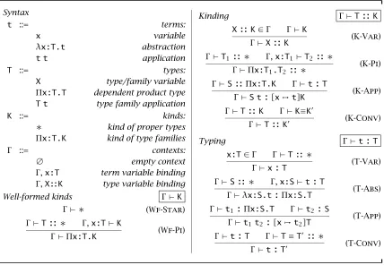
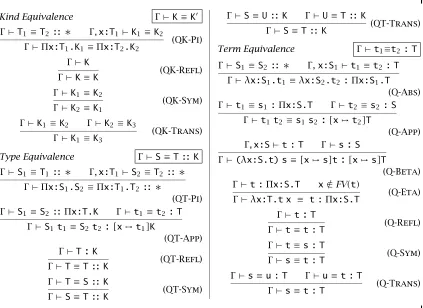
2 Dependent Types 45
David Aspinall and Martin Hofmann
2.1 Motivations 45
2.2 Pure First-Order Dependent Types 50 2.3 Properties 54
2.4 Algorithmic Typing and Equality 56 2.5 Dependent Sum Types 61
2.6 The Calculus of Constructions 64
3 Effect Types and Region-Based Memory Management 87
Fritz Henglein, Henning Makholm, and Henning Niss
3.1 Introduction and Overview 87 3.2 Value Flow by Typing with Labels 90 3.3 Effects 102
3.4 Region-Based Memory Management 106 3.5 The Tofte–Talpin Type System 114 3.6 Region Inference 123
3.7 More Powerful Models for Region-Based Memory
Management 127
3.8 Practical Region-Based Memory Management Systems 133
II Types for Low-Level Languages
137
4 Typed Assembly Language 141
Greg Morrisett
4.1 TAL-0: Control-Flow-Safety 142 4.2 The TAL-0 Type System 146 4.3 TAL-1: Simple Memory-Safety 155 4.4 TAL-1 Changes to the Type System 161 4.5 Compiling to TAL-1 164
4.6 Scaling to Other Language Features 167 4.7 Some Real World Issues 172
4.8 Conclusions 175
5 Proof-Carrying Code 177
George Necula
5.1 Overview of Proof Carrying Code 177 5.2 Formalizing the Safety Policy 182 5.3 Verification-Condition Generation 187 5.4 Soundness Proof 199
5.5 The Representation and Checking of Proofs 204 5.6 Proof Generation 214
Contents vii
III Types and Reasoning about Programs
221
6 Logical Relations and a Case Study in Equivalence Checking 223
Karl Crary
6.1 The Equivalence Problem 224
6.2 Non-Type-Directed Equivalence Checking 225 6.3 Type-Driven Equivalence 227
6.4 An Equivalence Algorithm 228 6.5 Completeness: A First Attempt 232 6.6 Logical Relations 233
6.7 A Monotone Logical Relation 236
6.8 The Main Lemma 237
6.9 The Fundamental Theorem 239
6.10 Notes 243
7 Typed Operational Reasoning 245
Andrew Pitts
7.1 Introduction 245
7.2 Overview 246
7.3 Motivating Examples 247 7.4 The Language 253
7.5 Contextual Equivalence 261
7.6 An Operationally Based Logical Relation 266 7.7 Operational Extensionality 279
7.8 Notes 288
IV
Types for Programming in the Large
291
8 Design Considerations for ML-Style Module Systems 293
Robert Harper and Benjamin C. Pierce
8.1 Basic Modularity 294
8.2 Type Checking and Evaluation of Modules 298 8.3 Compilation and Linking 302
8.4 Phase Distinction 305
8.5 Abstract Type Components 307 8.6 Module Hierarchies 317
8.7 Signature Families 320 8.8 Module Families 324 8.9 Advanced Topics 338
9 Type Definitions 347
Christopher A. Stone
9.1 Definitions in the Typing Context 351 9.2 Definitions in Module Interfaces 358 9.3 Singleton Kinds 367
9.4 Notes 384
V
Type Inference
387
10 The Essence of ML Type Inference 389
François Pottier and Didier Rémy
10.1 What Is ML? 389 10.2 Constraints 407 10.3 HM(X) 422
10.4 Constraint Generation 429 10.5 Type Soundness 434 10.6 Constraint Solving 438
10.7 From ML-the-Calculus to ML-the-Language 451
10.8 Rows 460
A Solutions to Selected Exercises 491
References 535
Preface
Overview
Work in type systems for programming languages now touches many parts of computer science, from language design and implementation to software engineering, network security, databases, and analysis of concurrent and dis-tributed systems. The aim of this book, together with its predecessor,Types and Programming Languages (Pierce [2002]—henceforthTAPL) is to offer a comprehensive and accessible introduction to the area’s central ideas, results, and techniques. The intended audience includes graduate students and re-searchers from other parts of computer science who want get up to speed in the area as a whole, as well as current researchers in programming languages who need comprehensible introductions to particular topics. UnlikeTAPL, the present volume is conceived not as a unified text, but as a collection of more or less separate articles, authored by experts on their particular topics.
Required Background
Most of the material should be accessible to readers with a solid grasp of the basic notations and techniques of operational semantics and type systems— roughly, the first half of TAPL. Some chapters depend on more advanced topics from the second half ofTAPLor earlier chapters of the present vol-ume; these dependencies are indicated at the beginning of each chapter. Inter-chapter dependencies have been kept to a minimum to facilitate reading in any order.
Topics
programs. The first,Substructural Type Systems,by David Walker, surveys type systems based on analogies with “substructural” logics such as linear logic, in which one or more of the structural rules of conventional logics— which allow dropping, duplicating, and permuting assumptions—are omitted or allowed only under controlled circumstances. In substructural type sys-tems, the type of a value is not only a description of its “shape,” but also a capability for using it a certain number of times; this refinement plays a key role in advanced type systems being developed for a range of purposes, including static resource management and analyzing deadlocks and livelocks in concurrent systems. The chapter onDependent Types, by David Aspinall and Martin Hofmann, describes a yet more powerful class of type systems, in which the behavior of computations on particular run-time values (not just generic “shapes”) may be described at the type level. Dependent type sys-tems blur the distinction between types and arbitrary correctness assertions, and between typechecking and theorem proving. The power of full dependent types has proved difficult to reconcile with language design desiderata such as automatic typechecking and the “phase distinction” between compile time and run time in compiled languages. Nevertheless, ideas of dependent typ-ing have played a fruitful role in language design and theory over the years, offering a common conceptual foundation for numerous forms of “indexed” type systems.Effect Types and Region-Based Memory Management, by Fritz Henglein, Henning Makholm, and Henning Niss, introduces yet another idea for extending the reach of type systems: in addition to describing the shape of an expression’s result (a static abstraction of the possible values that the expression may yield when evaluated), its type can also list a set of possible “effects,” abstracting the possible computational effects (mutations to the store, input and output, etc.) that its evaluation may engender. Perhaps the most sophisticated application of this idea has been in memory management systems based on static “region inference,” in which the effects manipulated by the typechecker track the program’s ability to read and write in particular regions of the heap. For example, the ML Kit Compiler used a region analy-sis internally to implement the full Standard ML language without a garbage collector.
Preface xi
compiler from a high-level language, through a series of typed intermedi-ate languages, down to this typed assembly code.Proof-Carrying Code, by George Necula, presents a more general formulation in a logical setting with close ties to the dependent types described in Aspinall and Hofmann’s chap-ter. The strength of this presentation is that it offers a natural transition from conventional type safety properties, such as memory safety, to more general security properties. A driving application area for both approaches is enforcing security guarantees when dealing with untrusted mobile code.
Types and Reasoning about Programs One attraction of rich type systems is that they support powerful methods of reasoning about programs—not only by compilers, but also by humans. One of the most useful, the tech-nique oflogical relations, is introduced in the chapterLogical Relations and a Case Study in Equivalence Checking, by Karl Crary. The extended example— proving the correctness of an algorithm for deciding a type-sensitive behav-ioral equivalence relation on terms in the simply typed lambda-calculus with a Unit type—foreshadows ideas developed further in Christopher Stone’s chapter on type definitions.Typed Operational Reasoning, by Andrew Pitts, develops a more general theory of typed reasoning about program equiv-alence. Here the examples focus on proving representation independence properties for abstract data types in the setting of a rich language combin-ing the universal and existential polymorphism of System F with records and recursive function definitions.
Types for Programming in the Large One of the most important projects in languagedesignover the past decade and more has been the use of type-theory as a framework for the design of sophisticated module systems— languages for assembling large software systems from modular components. One highly developed line of work is embodied in the module systems found in modern ML dialects.Design Considerations for ML-Style Module Systems, by Robert Harper and Benjamin C. Pierce, offers an informal guided tour of the principal features of this class of module systems—a “big picture” intro-duction to a large but highly technical body of papers in the research litera-ture.Type Definitions, by Christopher A. Stone, addresses the most critical and technically challenging feature of the type systems on which ML-style module systems are founded:singleton kinds, which allow type definitions to be internalized rather than being treated as meta-level abbreviations.
has for decades been a showcase for advances in typed language design and compiler implementation, and for the advantages of software construction in richly typed languages. One of the main reasons for the success of these lan-guages is the combination of power and convenience offered by their type inference (or type reconstruction) algorithms. Basic ML type inference has been described in many places, but descriptions of the more advanced tech-niques used in production compilers for full-blown languages have until now been widely dispersed in the literature, when they were available at all. In The Essence of ML Type Inference, François Pottier and Didier Rémy offer a comprehensive, unified survey of the area.
Exercises
Most chapters include numerous exercises. The estimated difficulty of each exercise is indicated using the following scale:
« Quick check 30 seconds to 5 minutes
«« Easy ≤1 hour
««« Moderate ≤3 hours
«««« Challenging >3 hours
Exercises marked«are intended as real-time checks of important concepts. Readers are strongly encouraged to pause for each one of these before mov-ing on to the material that follows. Some of the most important exercises are labeledRecommended.
Solutions to most of the exercises are provided in Appendix A. To save readers searching for solutions to exercises for which solutions are not avail-able, these are marked3.
Electronic Resources
Additional materials associated with this book can be found at:
http://www.cis.upenn.edu/~bcpierce/attapl
Resources available on this site will include errata for the text, pointers to supplemental material contributed by readers, and implementations associ-ated with various chapters.
Acknowledgments
Preface xiii
Derek Dreyer, Matthias Felleisen, Robby Findler, Kathleen Fisher, Nadji Gau-thier, Michael Hicks, Steffen Jost, Xavier Leroy, William Lovas, Kenneth Mac-Kenzie, Yitzhak Mandelbaum, Martin Müller, Simon Peyton Jones, Norman Ramsey, Yann Régis-Gianas, Fermin Reig, Don Sannella, Alan Schmitt, Peter Sewell, Vincent Simonet, Eijiro Sumii, David Swasey, Joe Vanderwaart, Yanling Wang, Keith Wansbrough, Geoffrey Washburn, Stephanie Weirich, Dinghao Wu, and Karen Zee for helping to make this a much better book than we could have done alone. Stephanie Weirich deserves a particularly warm round of thanks for numerous and incisive comments on the whole manuscript. Nate Foster’s assistance with copy editing, typesetting, and indexing contributed enormously to the book’s final shape.
P a r t I
1
Substructural Type Systems
David Walker
Advanced type systems make it possible to restrict access to data structures and to limit the use of newly-defined operations. Oftentimes, this sort of access control is achieved through the definition of new abstract types under control of a particular module. For example, consider the following simplified file system interface.
type file
val open : string → file option val read : file → string * file val append : file * string → file val write : file * string → file val close : file → unit
By declaring that the type fileis abstract, the implementer of the module can maintain strict control over the representation of files. A client has no way to accidentally (or maliciously) alter any of the file’s representation invariants. Consequently, the implementer may assume that the invariants that he or she establishes upon opening a file hold before anyread,append,writeor close.
While abstract types are a powerful means of controlling the structure of data, they are not sufficient to limit theorderingandnumber of usesof func-tions in an interface. Try as we might, there is no (static) way to prevent a file from being read after it has been closed. Likewise, we cannot stop a client from closing a file twice or forgetting to close a file.
resources such as files, locks and memory. Each of these resources undergoes a series of changes of state throughout its lifetime. Files, as we have seen, may be open or closed; locks may be held or not; and memory may be allocated or deallocated. Substructural type systems provide sound static mechanisms for keeping track of just these sorts of state changes and preventing operations on objects in an invalid state.
The bulk of this chapter will focus on applications of substructural type systems to the control of memory resources. Memory is a pervasive resource that must be managed carefully in any programming system so it makes an excellent target of study. However, the general principles that we establish can be applied to other sorts of resources as well.
1.1
Structural Properties
Most of the type systems in this book allowunrestricteduse of variables in the type checking context. For instance, each variable may be used once, twice, three times, or not at all. A precise analysis of the properties of such variables will suggest a whole new collection of type systems.
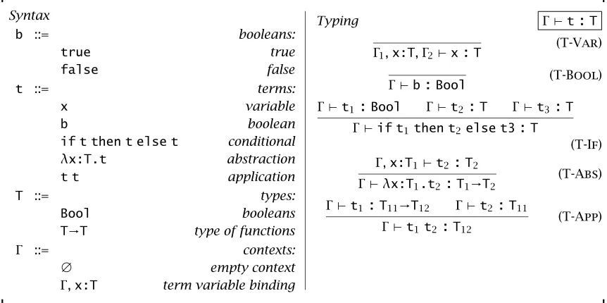
To begin our exploration, we will analyze the simply-typed lambda calcu-lus, which is reviewed in Figure 1-1. In this discussion, we are going to be particularly careful when it comes to the form of the type-checking contextΓ. We will consider such contexts to be simple lists of variable-type pairs. The "," operator appends a pair to the end of the list. We also write (Γ1, Γ2) for
the list that results from appendingΓ2 onto the end of Γ1. As usual, we
al-low a given variable to appear at most once in a context and to maintain this invariant, we implicitly alpha-convert bound variables before entering them into the context.
We are now in position to consider three basic structuralproperties sat-isfied by our simply-typed lambda calculus. The first property, exchange, indicates that the order in which we write down variables in the context is irrelevant. A corollary of exchange is that if we can type check a term with the contextΓ, then we can type check that term with any permutation of the variables inΓ. The second property,weakening, indicates that adding extra, unneeded assumptions to the context, does not prevent a term from type checking. Finally, the third property,contraction, states that if we can type check a term using two identical assumptions (x2:T1andx3:T1) then we can
check the same term using a single assumption.
1.1.1 Lemma [Exchange]: IfΓ1,x1:T1,x2:T2,Γ2`t:Tthen
Γ1,x2:T2,x1:T1,Γ2`t:T 2
1.1 Structural Properties 5
Syntax
b ::= booleans:
true true
false false
t ::= terms:
x variable
b boolean
if t then t else t conditional
λx:T.t abstraction
t t application
T ::= types:
Bool booleans
T→T type of functions
Γ ::= contexts:
∅ empty context
Γ,x:T term variable binding
Typing Γ`t:T
Γ1,x:T,Γ2`x:T
(T-Var)
Γ`b:Bool (T-Bool)
Γ`t1:Bool Γ`t2:T Γ`t3:T Γ`if t1then t2else t3:T
(T-If)
Γ,x:T1`t2:T2 Γ`λx:T1.t2:T1→T2
(T-Abs)
Γ `t1:T11→T12 Γ `t2:T11 Γ`t1t2:T12
[image:20.576.74.505.73.288.2](T-App)
Figure 1-1: Simply-typed lambda calculus with booleans
1.1.3 Lemma [Contraction]: IfΓ1,x2:T1,x3:T1,Γ2`t:T2then
Γ1,x1:T1,Γ2`[x2,x1][x3,x1]t:T2 2
1.1.4 Exercise [Recommended,«]: Prove that exchange, weakening and contrac-tion lemmas hold for the simply-typed lambda calculus. 2
Asubstructural type systemis any type system that is designed so that one or more of the structural properties do not hold. Different substructural type systems arise when different properties are withheld.
• Linear type systems ensure that every variable is used exactly once by allowing exchange but not weakening or contraction.
• Affine type systems ensure that every variable is used at most once by allowing exchange and weakening, but not contraction.
• Relevanttype systems ensure that every variable is used at least once by allowing exchange and contraction, but not weakening.
The picture below can serve as a mnemonic for the relationship between these systems. The system at the bottom of the diagram (the ordered type sys-tem) admits no structural properties. As we proceed upwards in the diagram, we add structural properties: E stands for exchange; W stands for weakening; and C stands for contraction. It might be possible to define type systems con-taining other combinations of structural properties, such as contraction only or weakening only, but so far researchers have not found applications for such combinations. Consequently, we have excluded them from the diagram.
ordered (none) linear (E)
affine (E,W) relevant (E,C)
unrestricted (E,W,C)
The diagram can be realized as a relation between the systems. We say system q1is more restrictive than systemq2and writeq1vq2when systemq1exhibits
fewer structural rules than systemq2. Figure 1-2 specifies the relation, which
we will find useful in the coming sections of this chapter.
1.2
A Linear Type System
1.2 A Linear Type System 7
q ::= system:
ord ordered
lin linear
rel relevant
aff affine
un unrestricted
ordvlin (Q-OrdLin)
linvrel (Q-LinRel)
linvaff (Q-LinAff)
relvun (Q-RelUn)
affvun (Q-AffUn)
qvq (Q-Reflex)
q1vq2 q2vq3
q1vq3
(Q-Trans)
Figure 1-2: A relation between substructural type systems
Syntax
Figure 1-3 presents the syntax of our linear language, which is an extension of the simply-typed lambda calculus. The main addition to be aware of, at this point, are the type qualifiersqthat annotate the introduction forms for all data structures. The linear qualifier (lin) indicates that the data structure in question will beused(i.e., appear in the appropriate elimination form) ex-actly once in the program. Operationally, we deallocate these linear values immediately after they are used. The unrestricted qualifier (un) indicates that the data structure behaves as in the standard simply-typed lambda calculus. In other words, unrestricted data can be used as many times as desired and its memory resources will be automatically recycled by some extra-linguistic mechanism (a conventional garbage collector).
Apart from the qualifiers, the only slightly unusual syntactic form is the elimination form for pairs. The termsplit t1as x,y in t2projects the first
and second components from the pairt1and calls themxandyint2. This
split operation allows us to extract two components while only counting a single use of a pair. Extracting two components using the more conven-tional projectionsπ1t1andπ2t1requires two uses of the pairt1. (It is also
possible, but a bit tricky, to provide the conventional projections.)
Syntax
q ::= qualifiers:
lin linear
un unrestricted
b ::= booleans:
true true
false false
t ::= terms:
x variable
q b boolean
if t then t else t conditional
q <t,t> pair
split t as x,y in t split
qλx:T.t abstraction
t t application
P ::= pretypes:
Bool booleans
T*T pairs
T→T functions
T ::= types:
q P qualified pretype
Γ ::= contexts:
∅ empty context
Γ,x:T term variable binding
Figure 1-3: Linear lambda calculus: Syntax
declarations, value declarations and let expressions where convenient; they all have the obvious meanings.
Typing
To ensure that linear objects are used exactly once, our type system maintains two important invariants.
1. Linear variables are used exactly once along every control-flow path.
2. Unrestricted data structures may not contain linear data structures. More generally, data structures with less restrictive type may not contain data structures with more restrictive type.
To understand why these invariants are useful, consider what could hap-pen if either invariant is broken. When considering the first invariant, as-sume we have constructed a functionfree that uses its argument and then deallocates it. Now, if we allow a linear variable (say x) to appear twice, a programmer might write<free x,free x>, or, slightly more deviously,
(λz.λy.<free z,free y>) x x.
In either case, the program ends up attempting to use and then freexafter it has already been deallocated, causing the program to crash.
1.2 A Linear Type System 9
Context Split Γ=Γ1◦Γ2 ∅ = ∅ ◦ ∅ (M-Empty)
Γ=Γ1◦Γ2
Γ,x:un P=(Γ1,x:un P)◦(Γ2,x:un P)
(M-Un)
Γ=Γ1◦Γ2
Γ,x:lin P=(Γ1,x:lin P)◦Γ2
(M-Lin1)
Γ=Γ1◦Γ2
Γ,x:lin P=Γ1◦(Γ2,x:lin P)
[image:24.576.72.509.70.146.2](M-Lin2)
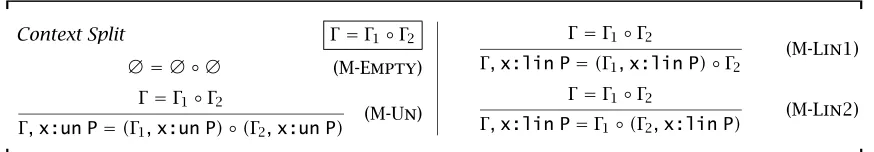
Figure 1-4: Linear lambda calculus: Context splitting
get exactly the same effect as above by using the unrestricted data structure multiple times:
let z = un <x,3> in split z as x1,_ in split z as x2,_ in <free x1,free x2>
Fortunately, our type system ensures that none of these situations can occur. We maintain the first invariant through careful context management. When type checking terms with two or more subterms, we pass all of the unre-stricted variables in the context to each subterm. However, we split the linear variables between the different subterms to ensure each variable is used ex-actly once. Figure 1-4 defines a relation,Γ =Γ1◦Γ2, which describes how to
split a single context in a rule conclusion (Γ) into two contexts (Γ1andΓ2) that
will be used to type different subterms in a rule premise.
To check the second invariant, we define the predicateq(T)(and its exten-sion to contextsq(Γ)) to express the typesTthat can appear in aq-qualified data structure. These containment rules state that linear data structures can hold objects with linear or unrestricted type, but unrestricted data structures can only hold objects with unrestricted type.
• q(T)if and only ifT = q0Pandqvq0
• q(Γ)if and only if(x:T)∈Γ impliesq(T)
Recall, we have already definedqvq0such that it is reflexive, transitive and linvun.
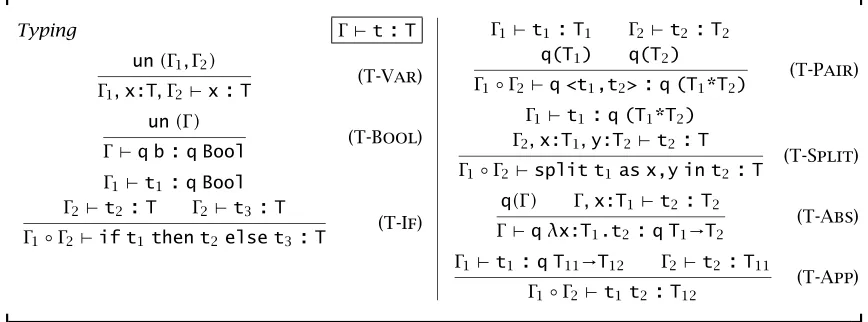
Now that we have defined the rules for containment and context splitting, we are ready for the typing rules proper, which appear in Figure 1-5. Keep in mind that these rules are constructed anticipating a call-by-value operational semantics.
Typing Γ`t:T un(Γ1,Γ2)
Γ1,x:T,Γ2`x:T
(T-Var)
un(Γ)
Γ `q b:q Bool (T-Bool)
Γ1`t1:q Bool Γ2`t2:T Γ2`t3:T Γ1◦Γ2`if t1then t2else t3:T
(T-If)
Γ1`t1:T1 Γ2`t2:T2
q(T1) q(T2)
Γ1◦Γ2`q <t1,t2>:q (T1*T2)
(T-Pair)
Γ1`t1:q (T1*T2) Γ2,x:T1,y:T2`t2:T Γ1◦Γ2`split t1as x,y in t2:T
(T-Split)
q(Γ) Γ,x:T1`t2:T2
Γ `qλx:T1.t2:q T1→T2
(T-Abs)
Γ1`t1:q T11→T12 Γ2`t2:T11 Γ1◦Γ2`t1t2:T12
[image:25.576.68.502.72.233.2](T-App)
Figure 1-5: Linear lambda calculus: Typing
in substructural type systems these cases have a special role in defining the nature of the type system, and subtle changes can make all the difference. In our linear system, the base cases must ensure that no linear variable is discarded without being used. To enforce this invariant in rule (T-Var), we explicitly check thatΓ1andΓ2contain no linear variables using the condition
un(Γ1,Γ2). We make a similar check in rule(T-Bool). Notice also that rule
(T-Var) is written carefully to allow the variablex to appear anywhere in the context, rather than just at the beginning or at the end.
1.2.1 Exercise [«]: What is the effect of rewriting the variable rule as follows? un(Γ)
Γ,x:T`x:T (T-BrokenVar)
The inductive cases of the typing relation take care to use context splitting to partition linear variables between various subterms. For instance, rule (T-If)splits the incoming context into two parts, one of which is used to check subtermt1and the other which is used to check botht2andt3. As a result,
a particular linear variable will occur once int2and once int3. However, the
linear object bound to the variable in question will be used (and hence de-allocated) exactly once at run time since only one oft2ort3will be executed.
1.2 A Linear Type System 11
unrestricted type. If we omitted this constraint, we could write the follow-ing badly behaved functions. (For clarity, we have retained the unrestricted qualifiers in this example rather than omitting them.)
type T = un (un bool → lin bool)
val discard = lin λx:lin bool.
(lin λf:T.lin true) (un λy:un bool.x)
val duplicate = lin λx:lin bool.
(lin λf:T.lin <f (un true),f (un true)>)) (un λy:un bool.x)
The first function discards a linear argumentxwithout using it and the sec-ond duplicates a linear argument and returns two copies of it in a pair. Hence, in the first case, we fail to deallocatexand in the second case, a subsequent function may project both elements of the pair and usextwice, which would result in a memory error asxwould be deallocated immediately after the first use. Fortunately, the containment constraint disallows the linear variablex from appearing in the unrestricted function(λy:bool. x).
Now that we have defined our type system, we should verify our intended structural properties: exchange for all variables, and weakening and contrac-tion for unrestricted variables.
1.2.2 Lemma [Exchange]: IfΓ1,x1:T1,x2:T2,Γ2`t:Tthen
Γ1,x2:T2,x1:T1,Γ2`t:T. 2
1.2.3 Lemma [Unrestricted Weakening]: IfΓ`t:Tthen
Γ,x1:un P1`t:T. 2
1.2.4 Lemma [Unrestricted Contraction]: IfΓ,x2:un P1,x3:un P1`t:T3then
Γ,x1:un P1`[x2,x1][x3,x1]t:T3. 2
Proof: The proofs of all three lemmas follow by induction on the structure
of the appropriate typing derivation. 2
Algorithmic Linear Type Checking
Algorithmic Typing Γin`t:T;Γout
Γ1,x:un P,Γ2`x:un P;Γ1,x:un P,Γ2
(A-UVar)
Γ1,x:lin P,Γ2`x:lin P;Γ1,Γ2 (A-LVar) Γ`q b:q Bool;Γ (A-Bool)
Γ1`t1:q Bool;Γ2 Γ2`t2:T;Γ3 Γ2`t3:T;Γ3 Γ1`if t1then t2else t3:T;Γ3
(A-If)
Γ1`t1:T1;Γ2 Γ2`t2:T2;Γ3
q(T1) q(T2)
Γ1`q <t1,t2>:q (T1*T2);Γ3
(A-Pair)
Γ1`t1:q (T1*T2);Γ2 Γ2,x:T1,y:T2`t2:T;Γ3 Γ1`split t1as x,y in t2:
T;Γ3÷(x:T1,y:T2)
(A-Split)
q=un⇒Γ1=Γ2÷(x:T1) Γ1,x:T1`t2:T2;Γ2
Γ1`qλx:T1.t2:q T1→T2;Γ2÷(x:T1)
(A-Abs)
Γ1`t1:q T11→T12;Γ2 Γ2`t2:T11;Γ3 Γ1`t1t2:T12;Γ3
[image:27.576.73.505.74.243.2](A-App)
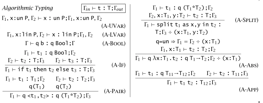
Figure 1-6: Linear lambda calculus: Algorithmic type checking
Γ=Γ1◦Γ2, we must guess how to split an input contextΓ into two parts.
For-tunately, it is relatively straightforward to restructure the type checking rules to avoid having to make these guesses. This restructuring leads directly to a practical type checking algorithm.
The central idea is that rather than splitting the context into parts before checking a complex expression composed of several subexpressions, we can pass the entire context as an input to the first subexpression and have it return the unused portion as an output. This output may then be used to check the next subexpression, which may also return some unused portions of the context as an output, and so on. Figure 1-6 makes these ideas concrete. It defines a new algorithmic type checking judgment with the form Γin `
t : T;Γout, where Γin is the input context, some portion of which will be
consumed during type checking of t, andΓout is the output context, which
will be synthesized alongside the typeT.
There are several key changes in our reformulated system. First, the base cases for variables and constants allow any context to pass through the judg-ment rather than restricting the number of linear variables that appear. In order to ensure that linear variables are used, we move these checks to the rules where variables are introduced. For instance, consider the rule(A-Split). The second premise has the form
Γ2,x:T1,y:T2`t2:T;Γ3
IfT1andT2are linear, then they should be used int2and should not appear
1.2 A Linear Type System 13
inΓ3, but we should delete them from the final outgoing context of the rule
so that the ordinary scoping rules for the variables are enforced. To handle both the check that linear variables do not appear and the removal of unre-stricted variables, we use a special “context difference” operator (÷). Using this operator, the final outgoing context of the rule(A-Split)is defined to be
Γ3÷(x:T1,y:T2). Formally, context difference is defined as follows.
Γ÷ ∅ =Γ
Γ1÷Γ2=Γ3 (x:lin P)6∈Γ3 Γ1÷(Γ2,x:lin P)=Γ3
Γ1÷Γ2=Γ3 Γ3=Γ4,x:un P,Γ5 Γ1÷(Γ2,x:un P)=Γ4,Γ5
Notice that this operator is undefined when we attempt to take the dif-ference of two contexts,Γ1 andΓ2, that contain bindings for the same linear
variable (x:lin P). If the undefined quotientΓ1÷Γ2were to appear anywhere
in a typing rule, the rule itself would not be considered defined and could not be part of a valid typing derivation.
The rule for abstraction(A-Abs)also introduces a variable and hence it also uses context difference to manipulate the output context for the rule. Ab-stractions must also satisfy the appropriate containment conditions. In other words, rule (A-Abs)must check that unrestricted functions do not contain linear variables. We perform this last check by verifying that when the func-tion qualifier is unrestricted, the input and output contexts from checking the function body are the same. This equivalence check is sufficient because if a linear variable was used in the body of an unrestricted function (and hence captured in the function closure), that linear variable would not show up in the outgoing context.
It is completely straightforward to check that every rule in our algorithmic system is syntax directed and that all our auxiliary functions including con-text membership tests and concon-text difference are easily computable. Hence, we need only show that our algorithmic system is equivalent to the simpler and more elegant declarative system specified in the previous section. The proof of equivalence can be a broken down into the two standard compo-nents:soundnessandcompletenessof the algorithmic system with respect to the declarative system. However, before we can get to the main results, we will need to show that our algorithmic system satisfies some basic structural properties of its own. In the following lemmas, we use the notationL(Γ)and
1.2.5 Lemma [Algorithmic Monotonicity]: IfΓ `t : T;Γ0 then U(Γ0) = U(Γ)
andL(Γ0)⊆ L(Γ). 2
1.2.6 Lemma [Algorithmic Exchange]: If Γ1, x1:T1, x2:T2, Γ2 ` t : T;Γ3 then Γ1,x2:T2,x1:T1,Γ2`t:T;Γ30andΓ3is the same asΓ30up to transposition of
the bindings forx1andx2. 2
1.2.7 Lemma [Algorithmic Weakening]: If Γ ` t : T;Γ0 then Γ, x:T0 ` t : T;
Γ0,x:T0. 2
1.2.8 Lemma [Algorithmic Linear Strengthening]: If Γ, x:lin P ` t : T;
Γ0,x:lin PthenΓ`t:T;Γ0. 2
Each of these lemmas may be proven directly by induction on the initial typing derivation. The algorithmic system also satisfies a contraction lemma, but since it will not be necessary in the proofs of soundness and complete-ness, we have not stated it here.
1.2.9 Theorem [Algorithmic Soundness]: IfΓ1 ` t: T;Γ2 and L(Γ2) = ∅ then
Γ1`t:T. 2
Proof: As usual, the proof is by induction on the typing derivation. The struc-tural lemmas we have just proven are required to push through the result, but
it is mostly straightforward. 2
1.2.10 Theorem [Algorithmic Completeness]: If Γ1 ` t : T then Γ1 ` t : T;Γ2
andL(Γ2)= ∅. 2
Proof: The proof is by induction on the typing derivation. 2
Operational Semantics
To make the memory management properties of our language clear, we will evaluate terms in an abstract machine with an explicit store. As indicated in Figure 1-7, stores are a sequence of variable-value pairs. We will implicitly assume that any variable appears at most once on the left-hand side of a pair so the sequence may be treated as a finite partial map.
A value is a pair of a qualifier together with some data (aprevaluew). For the sake of symmetry, we will also assume that all values are stored, even base types such as booleans. As a result, both components of any pair will be pointers (variables).
1.2 A Linear Type System 15
w ::= prevalues:
b boolean
<x,y> pair
λx:T.t abstraction
v ::= values:
q w qualified prevalue
S ::= stores:
∅ empty context
S,x,v store binding
E ::= evaluation contexts:
[ ] context hole
if E then t else t if context
q <E,t> fst context
q <x,E> snd context
split E as x,y in t split context
E t fun context
x E arg context
Figure 1-7: Linear lambda calculus: Run-time data
are terms with a single hole. Contexts define the order of evaluation of terms— they specify the places in a term where a computation can occur. In our case, evaluation is left-to-right since, for example, there is a context with the form E tindicating that we can reduce the term in the function position before re-ducing the term in the argument position. However, there is no context with the formt E. Instead, there is only the more limited contextx E, indicating that we must reduce the term in the function position to a pointerxbefore proceeding to evaluate the term in the argument position. We use the nota-tionE[t]to denote the term composed of the contextEwith its hole plugged by the computationt.
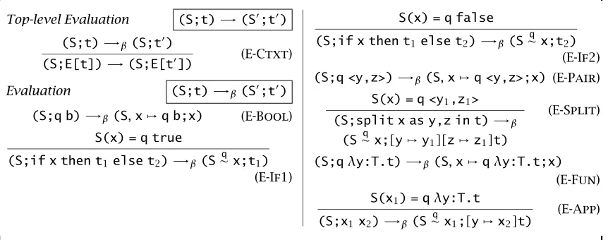
The operational semantics, defined in Figure 1-8, is factored into two re-lations. The first relation,(S;t) -→(S0;t0), picks out a subcomputation to evaluate. The second relation,(S;t) -→β(S0;t0), does all the real work. In
order to avoid creation of two sets of operational rules, one for linear data, which is deallocated when used, and one for unrestricted data, which is never deallocated, we define an auxiliary function,S∼q x, to manage the differences.
(S1,x,v,S2)lin∼ x = S1,S2
Sun∼x = S
Aside from these details, the operational semantics is standard.
Preservation and Progress
Top-level Evaluation (S;t) -→(S0;t0)
(S;t) -→β(S;t0)
(S;E[t]) -→(S;E[t0]) (E-Ctxt)
Evaluation (S;t) -→β(S0;t0)
(S;q b) -→β(S,x,q b;x) (E-Bool)
S(x) = q true
(S;if x then t1else t2) -→β(S∼q x;t1)
(E-If1)
S(x) = q false
(S;if x then t1else t2) -→β(S∼q x;t2)
(E-If2) (S;q <y,z>) -→β(S,x,q <y,z>;x) (E-Pair)
S(x) = q <y1,z1>
(S;split x as y,z in t) -→β
(S∼q x;[y,y1][z,z1]t)
(E-Split)
(S;qλy:T.t) -→β(S,x,qλy:T.t;x)
(E-Fun) S(x1) = qλy:T.t
(S;x1x2) -→β(S∼q x1;[y,x2]t)
[image:31.576.72.503.74.244.2](E-App)
Figure 1-8: Linear lambda calculus: Operational semantics
implementation, we will extend the declarative typing rules rather than the algorithmic typing rules.
Figure 1-9 presents the machine typing rules in terms of two judgments, one for stores and the other for programs. The store typing rules generate a context that describes the available bindings in the store. The program typ-ing rule uses the generated bindtyp-ings to check the expression that will be executed.
With this new machinery in hand, we are able to prove the standard progress and preservation theorems.
1.2.11 Theorem [Preservation]: If ` (S;t) and (S;t) -→ (S0;t0) then
`(S0;t0). 2
1.2.12 Theorem [Progress]: If`(S;t)then(S;t) -→(S0;t0)ortis a value. 2
1.2.13 Exercise [Recommended,«]: You will need a substitution lemma to com-plete the proof of preservation. Is the following the right one?
Conjecture: Let Γ3 = Γ1◦Γ2. If Γ1, x:T ` t1 : T1 and Γ2 ` t : T then
Γ3`[x,t]t1:T1. 2
1.2.14 Exercise [«««,3]: Prove progress and preservation usingTAPL, Chapters 9
1.3 Extensions and Variations 17
Store Typing `S:Γ
` ∅:∅ (T-EmptyS)
`S:Γ1◦Γ2 Γ1`lin w:T `S,x,lin w:Γ2,x:T
(T-NextlinS)
`S:Γ1◦Γ2 Γ1`un w:T `S,x,un w:Γ2,x:T
(T-NextunS)
Program Typing `(S;t)
`S:Γ Γ`t:T
`(S;t) (T-Prog)
Figure 1-9: Linear lambda calculus: Program typing
1.3
Extensions and Variations
Most features found in modern programming languages can be defined to interoperate successfully with linear type systems, although some are trickier than others. In this section, we will consider a variety of practical extensions to our simple linear lambda calculus.
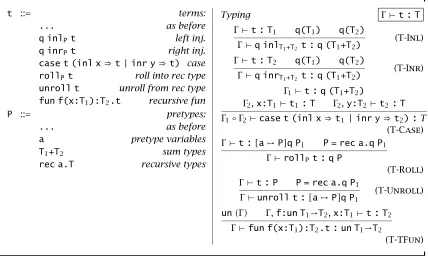
Sums and Recursive Types
Complex data structures, such as the recursive data types found in ML-like languages, pose little problem for linear languages. To demonstrate the cen-tral ideas involved, we extend the syntax for the linear lambda calculus with the standard introduction and elimination forms for sums and recursive types. The details are presented in Figure 1-10.
Values with sum type are introduced by injections q inlPt or q inrPt, wherePisT1+T2, the resulting pretype of the term. In the first instance, the
underlying termtmust have typeT1, and in the second instance, the
under-lying termtmust have typeT2. The qualifierqindicates the linearity of the
argument in exactly the same way as for pairs. The case expression will exe-cute its first branch if its primary argument is a left injection and its second branch if its primary argument is a right injection. We assume that+binds more tightly that→but less tightly than*.
t ::= terms:
... as before
q inlPt left inj.
q inrPt right inj.
case t (inl x⇒t | inr y⇒t) case
rollPt roll into rec type unroll t unroll from rec type
fun f(x:T1):T2.t recursive fun
P ::= pretypes:
... as before
a pretype variables
T1+T2 sum types
rec a.T recursive types
Typing Γ`t:T
Γ`t:T1 q(T1) q(T2) Γ `q inlT1+T2 t:q (T1+T2)
(T-Inl)
Γ`t:T2 q(T1) q(T2) Γ `q inrT1+T2 t:q (T1+T2)
(T-Inr)
Γ1`t:q (T1+T2)
Γ2,x:T1`t1:T Γ2,y:T2`t2:T Γ1◦Γ2`case t (inl x⇒t1| inr y⇒t2):T
(T-Case)
Γ`t:[a,P]q P1 P = rec a.q P1 Γ`rollPt:q P
(T-Roll)
Γ`t:P P = rec a.q P1 Γ`unroll t:[a,P]q P1
(T-Unroll)
un(Γ) Γ,f:un T1→T2,x:T1`t:T2
Γ`fun f(x:T1):T2.t:un T1→T2
[image:33.576.74.502.73.329.2](T-TFun)
Figure 1-10: Linear lambda calculus: Sums and recursive types
of sums and recursive types, we will normally omit the typing annotations on their introduction forms in our examples.
In order to write computations that process recursive types, we add recur-sive function declarations to our language as well. Since the free variables in a recursive function closure will be used on each recursive invocation of the function, we cannot allow the closure to contain linear variables. Hence, all recursive functions are unrestricted data structures.
A simple but useful data structure is the linear list ofTs:
type T llist = rec a.lin (unit + lin (T * lin a))
Here, the entire spine (aside from the terminating value of unit type) is linear while the underlyingTobjects may be linear or unrestricted. To create a fully unrestricted list, we simply omit the linear qualifiers on the sum and pairs that make up the spine of the list:
1.3 Extensions and Variations 19
After defining the linear lists, the memory conscious programmer can write many familiar list-processing functions in a minimal amount of space. For example, here is how we map an unrestricted function across a linear list. Remember, multi-argument functions are abbreviations for functions that ac-cept linear pairs as arguments.
fun nil(_:unit) : T2 llist =
roll (lin inl ())
fun cons(hd:T2, tl:T2 llist) : T2 llist =
roll (lin inr (lin <hd,tl>))
fun map(f:T1→T2, xs:T1 llist) : T2 llist =
case unroll xs ( inl _ ⇒ nil() | inr xs ⇒
split xs as hd,tl in cons(f hd,map lin <f,tl>))
In this implementation ofmap, we can observe that on each iteration of the loop, it is possible to reuse the space deallocated bysplitorcaseoperations for the allocation operations that follow in the body of the function (inside the calls tonilandcons).
Hence, at first glance, it appears thatmapwill execute with only a constant space overhead. Unfortunately, however, there are some hidden costs asmap executes. A typical implementation will store local variables and temporaries on the stack before making a recursive call. In this case, the result off hdwill be stored on the stack while map iterates down the list. Consequently, rather than having a constant space overhead, our map implementation will have an O(n) overhead, wherenis the length of the list. This is not too bad, but we can do better.
In order to do better, we need to avoid implicit stack allocation of data each time we iterate through the body of a recursive function. Fortunately, many functional programming languages guarantee that if the last operation in a function is itself a function call then the language implementation will deallocate the current stack frame before calling the new function. We name such function calls tail calls and we say that any language implementation that guarantees that the current stack frame will be deallocated before a tail call istail-call optimizing.
output list will wind up in reverse order, so we will reverse it at the end. Both of the loops in the code, mapRev and reverseare tail-recursivefunctions. That is, they end in a tail call and have a space-efficient implementation.
fun map(f:T1→T2, input:T1 llist) : T2 llist =
reverse(mapRev(f,input,nil()),nil())
and mapRev(f:T1→T2,
input:T1 llist,
output:T2 llist) : T2 llist =
case unroll input ( inl _ ⇒ output | inr xs ⇒
split xs as hd,tl in
mapRev (f,tl,cons(f hd,output)))
and reverse(input:T2 llist, output:T2 llist)
case unroll input ( inl _ ⇒ output | inr xs ⇒
split xs as hd,tl in
reverse(tl,cons(hd,output)))
This link reversal algorithm is a well-known way of traversing a list in constant space. It is just one of a class of algorithms developed well before the invention of linear types. A similar algorithm was invented by Deutsch, Schorr, and Waite for traversing trees and graphs in constant space. Such con-stant space traversals are essential parts of mark-sweep garbage collectors— at garbage collection time there is no extra space for a stack so any traversal of the heap must be done in constant space.
1.3.1 Exercise [«««]: Define a recursive type that describes linear binary trees that hold data of typeTin their internal nodes (nothing at the leaves). Write a constant-space functiontreeMapthat produces an identically-shaped tree on output as it was given on input, modulo the action of the functionfthat is applied to each element of the tree. Feel free to use reasonable extensions to our linear lambda calculus including mutually recursive functions, n-ary
tuples and n-ary sums. 2
Polymorphism
1.3 Extensions and Variations 21
1. Reuse of code to perform the same algorithm, but on data with different shapes.
2. Reuse of code to perform the same algorithm, but on data governed by different memory management strategies.
To support the first kind of polymorphism, we will allow quantification over pretypes. To support the second kind of polymorphism, we will allow quantification over qualifiers. A good example of both sorts of polymorphism arises in the definition of a polymorphicmapfunction. In the code below, we useaandbto range over pretype variables as we did in the previous section, andpto range over qualifier variables.
type (p1,p2,a) list =
rec a.p1 (unit + p1 (p2 a * (p1,p2,a) list))
map :
∀a,b.
∀pa,pb.
lin ((pa a → pb b)*(lin,pa,a) list)→(lin,pb,b) list
The type definition in the first line defines lists in terms of three parameters. The first parameter,p1, gives the usage pattern (linear or unrestricted) for the
spine of the list, while the second parameter gives the usage pattern for the elements of the list. The third parameter is a pretype parameter, which gives the (pre)type of the elements of list. Themapfunction is polymorphic in the argument (a) and result (b) element types of the list. It is also polymorphic (via parameterspa andpb) in the way those elements are used. Overall, the
function maps lists with linear spines to lists with linear spines.
Developing a system for polymorphic, linear type inference is a challenging research topic, beyond the scope of this book, so we will assume that, unlike in ML, polymorphic functions are introduced explicitly using the syntaxΛa.t orΛp.t. Here,aandpare the type parameters to a function with bodyt. The body does not need to be a value, like in ML, since we will run the polymorphic function every time a pretype or qualifier is passed to the function as an argument. The syntaxt0[P]ort0[q]applies the functiont0to its pretype or qualifier argument. Figure 1-11 summarizes the syntactic extensions to the language.
q ::= qualifiers:
... as before
p polymorphic qualifier
t ::= terms:
... as before
qΛa.t pretype abstraction
t [P] pretype application
qΛp.t qualifier abstraction
t [q] qualifier application
P ::= pretypes:
... as before
∀a.T pretype polymorphism ∀p.T qualifier polymorphism
Figure 1-11: Linear lambda calculus: Polymorphism syntax
val nil : ∀a,p2.(lin,p2,a) list = Λa,p2.roll (lin inl ())
val list :
∀a,p2.lin (p2 a * (lin,p2,a) list)→(lin,p2,a) list = Λa,p2.
λcell : lin (p2 a * (lin,p2,a) list).
roll (lin inr (lin cell))
Now our most polymorphicmapfunction may be written as follows.
val map =
Λa,b. Λpa,pb.
fun aux(f:(pa a → pb b),
xs:(lin,pa,a) list)) : (lin,pb,b) list =
case unroll xs (
inl _ ⇒ nil [b,pb] ()
| inr xs ⇒ split xs as hd,tl in
cons [b,pb] (pb <f hd,map (lin <f,tl>)>))
In order to ensure that our type system remains sound in the presence of pretype polymorphism, we add the obvious typing rules, but change very little else. However, adding qualifier polymorphism, as we have done, is a little more involved. Before arriving at the typing rules themselves, we need to adapt some of our basic definitions to account for abstract qualifiers that may either be linear or unrestricted.
1.3 Extensions and Variations 23
Context Split Γ=Γ1◦Γ2
Γ=Γ1◦Γ2 Γ,x:p P=(Γ1,x:p P)◦Γ2
(M-Abs1)
Γ=Γ1◦Γ2
Γ,x:p P=Γ1◦(Γ2,x:p P)
(M-Abs2)
Figure 1-12: Linear context manipulation rules
∆ ::= type contexts:
∅ empty
∆,a pretype var.
∆,p qualifier var.
Typing ∆;Γ`t:T
q(Γ) ∆,a;Γ`t:T
∆;Γ `qΛa.t:q∀a.T (T-PAbs)
∆;Γ`t:q∀a.T FV(P)⊆∆
∆;Γ`t [P]:[a,P]T (T-PApp) q(Γ) ∆,p;Γ `t:T
∆;Γ`qΛp.t:q∀p.T (T-QAbs)
∆;Γ`t:q1∀p.T FV(q)⊆∆
∆;Γ`t [q]:[p,q]T (T-QApp)
Figure 1-13: Linear lambda calculus: Polymorphic typing
Second, we need to conservatively extend the relation on type qualifiers q1vq2 so that it is sound in the presence of qualifier polymorphism. Since
the linear qualifier is the least qualifier in the current system, the following rule should hold.
linvp (Q-LinP)
Likewise, sinceunis the greatest qualifier in the system, we can be sure the following rule is sound.
pvun (Q-PUn)
Aside from these rules, we will only be able to infer that an abstract qual-ifier p is related to itself via the general reflexivity rule. Consequently, lin-ear data structures can contain abstract ones; abstract data structures can contain unrestricted data structures; and data structure with qualifierpcan contain other data with qualifierp.
The typing rules for the other constructs we have seen are almost un-changed. One relatively minor alteration is that the incoming type context
∆will be propagated through the rules to account for the free type variables. Unlike term variables, type variables can always be used in an unrestricted fashion; it is difficult to understand what it would mean to restrict the use of a type variable to one place in a type or term. Consequently, all parts of∆ are propagated from the conclusion of any rule to all premises. We also need the occasional side condition to check that whenever a programmer writes down a type, its free variables are contained in the current type context∆. For instance the rules for function abstraction and application will now be written as follows.
q(Γ) FV(T1)⊆∆ ∆;Γ,x:T1`t2:T2
∆;Γ`qλx:T1.t2:q T1→T2
(T-Abs)
∆;Γ1`t1:q T1→T2 ∆;Γ2`t2:T1 ∆;Γ1◦Γ2`t1t2:T2
(T-App)
The most important way to test our system for faults is to prove the type substitution lemma. In particular, the proof will demonstrate that we have made safe assumptions about how abstract type qualifiers may be used.
1.3.2 Lemma [Type Substitution]:
1. If∆,p;Γ `t:TandFV(q)∈∆then∆;[p,q]Γ`[p,q]t:[p,q]T
2. If∆,a;Γ `t:TandFV(P)∈∆then∆;[a,P]Γ`[a,P]t:[a,P]T 2
1.3.3 Exercise [«]: Sketch the proof of the type substitution lemma. What
struc-tural rule(s) do you need to carry out the proof? 2
Operationally, we will choose to implement polymorphic instantiation us-ing substitution. As a result, our operational semantics changes very little. We only need to specify the new computational contexts and to add the eval-uation rules for polymorphic functions and application as in Figure 1-14.
Arrays
Arrays pose a special problem for linearly typed languages. If we try to pro-vide an operation fetches an element from an array in the usual way, perhaps using an array index expressiona[i], we would need to reflect the fact that theithelement (and only theithelement) of the array had been “used.”
1.3 Extensions and Variations 25
E ::= evaluation contexts:
E [P] pretype app context
E [q] qualifier app context
(S;qΛa.t) -→β(S,x,qΛa.t;x) (E-PFun)
S(x) = qΛa.t
(S;x [P]) -→β(S∼q x;[a,P]t)
(E-PApp)
(S;qΛp.t) -→β(S,x,qΛp.t;x) (E-QFun)
S(x) = qΛp.t
(S;x [q1]) -→β(S∼q x;[p,q1]t)
(E-QApp)
Figure 1-14: Linear lambda calculus: Polymorphic operational semantics
We dodged this problem when we constructed our tuple operations by defining a pattern matching construct that simultaneously extracted all of the elements of a tuple. Unfortunately, we cannot follow the same path for arrays because in modern languages like Java and ML, the length of an array (and therefore the size of the pattern) is unknown at compile time.
Another non-solution to the problem is to add a special built-in iterator to process all the elements in an array at once. However, this last prevents programmers from using arrays as efficient, constant-time, random-access data structures; they might as well use lists instead.
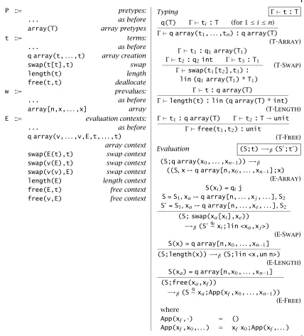
One way out of this jam is to design the central array access operations so that, unlike the ordinary “get” and “set” operations, theypreservethe number of pointers to the array and the number of pointers to each of its elements. We avoid our problem because there is no change to the array data structure that needs to be reflected in the type system. Using this idea, we will be able to allow programmers to define linear arrays that can hold a collection of arbitrarily many linear objects. Moreover, programmers will be able to access any of these linear objects, one at a time, using a convenient, constant-time, random-access mechanism.
In addition to swap, we provide functions to allocate an array given its list of elements (array), to determine array length (length) and to deallocate arrays (free). The last operation is somewhat unusual in that it takes two arguments a and f, where a is an array of type lin array(T) and f is a function with type T→unit that is run on each element ofT. The function may be thought of as a finalizer for the elements; it may be used to deallocate any linear components of the array elements, thereby preserving the single pointer property.
Our definition of arrays is compatible with the polymorphic system from the previous subsection, but for simplicity, we formalize it in the context of the simply-typed lambda calculus (see Figure 1-15).
1.3.4 Exercise [Recommended,«]: The typing rule for array allocation(T-Array) contains the standard containment check to ensure that unrestricted arrays cannot contain linear objects. What kinds of errors can occur if this check is
omitted? 2
1.3.5 Exercise [««,3]: With the presence of mutable data structures, it is possible to create cycles in the store. How should we modify the store typing rules to
take this into account? 2
The swap and free functions are relatively low-level operations. Fortu-nately, it is easy to build more convenient, higher-level abstractions out of them. For instance, the following code defines some simple functions for ma-nipulating linear matricies of unrestricted integers.
type iArray = lin array(int) type matrix = lin array(iArray)
fun dummy(x:unit):iArray = lin array()
fun freeElem(x:int):unit = ()
fun freeArray(a:iArray):unit = free(a,freeElem) fun freeMatrix(m:matrix):unit = free(m,freeArray)
fun get(a:matrix,i:int,j:int):lin (matrix * int) = split swap(a[i],dummy()) as a,b in
split swap(b[j],0) as b,k in split swap(b[j],k) as b,_ in split swap(a[i],b) as a,junk in freeArray(junk);
1.3 Extensions and Variations 27
P ::= pretypes:
... as before
array(T) array pretypes
t ::= terms:
... as before
q array(t,. . .,t) array creation
swap(t[t],t) swap
length(t) length
free(t,t) deallocate
w ::= prevalues:
... as before
array[n,x,. . .,x] array
E ::= evaluation contexts:
... as before
q array(v,. . .,v,E,t,. . .,t)
array context
swap(E(t),t) swap context
swap(v(E),t) swap context
swap(v(v),E) swap context
length(E) length context
free(E,t) free context
free(v,E) free context
Typing Γ`t:T
q(T) Γ`ti:T (for 1≤i≤n)
Γ`q array(t1,. . .,tn):q array(T)
(T-Array)
Γ `t1:q1array(T1) Γ`t2:q2int Γ`t3:T1
Γ `swap(t1[t2],t3):
lin (q1array(T1) * T1)
(T-Swap)
Γ`t:q array(T)
Γ`length(t):lin (q array(T) * int) (T-Length)
Γ`t1:q array(T) Γ`t2:T→unit Γ`free(t1,t2):unit
(T-Free)
Evaluation (S;t) -→β(S0;t0)
(S;q array(x0,. . .,xn−1)) -→β
((S,x,q array[n,x0,. . .,xn−1];x)
(E-Array) S(xi) = qij
S = S1,xa,q array[n,. . .,xj,. . .],S2
S0= S1,xa,q array[n,. . .,xe,. . .],S2
(S; swap(xa[xi],xe)) -→β(S0∼qixi;lin <xa,xj>)
(E-Swap) S(x) = q array[n,x0,. . .,xn−1]
(S;length(x)) -→β(S;lin <x,un n>)
(E-Length) S(xa) = q array[n,x0,. . .,xn−1]
(S;free(xa,xf))
-→β(S∼q xa;App(xf,x0,. . .,xn−1))
(E-Free) where
App(xf,·) = ()
[image:42.576.78.506.78.551.2]App(xf,x0,. . .) = xf x0;App(xf,. . .)
fun set(a:matrix,i:int,j:int,e:int):matrix = split swap(a[i],dummy()) as a,b in
split swap(b[j],e) as b,_ in split swap(a[i],b) as a,junk in freeArray(junk);
a
1.3.6 Exercise [««,3]: Use the functions provided above to write matrix-matrix multiply. Your multiply function should return an integer and deallocate both arrays in the process. Use any standard integer operations necessary. 2
In the examples above, we needed some sort of dummy value to swap into an array to replace the value we wanted to extract. For integers and arrays it was easy to come up with one. However, when dealing with polymorphic or abstract types, it may not be possible to conjure up a value of the right type. Consequently, rather than manipulating arrays with type q array(a) for some abstract typea, we may need to manipulate arrays of options with typeq array(a + unit). In this case, when we need to read out a value, we always have another value (inr ()) to swap in in its place. Normally such operations are calleddestructive reads; they are a common way to preserve the single pointer property when managing complex structured data.
Reference Counting
Array swaps and destructive reads are dynamic techniques that can help over-come a lack of compile-time knowledge about the number of uses of a par-ticular object.Reference countingis another dynamic technique that serves a similar purpose. Rather than restricting the number of pointers to an object to be exactly one, we can allow any number of pointers to the object and keep track of that number dynamically. Only when the last reference is used will the object be deallocated.
1.3 Extensions and Variations 29
Syntax
q ::= qualifiers:
... as before
rc ref. count
t ::= terms:
... as before
inc(t) increment count
dec(t,t) decrement count
Qualifier Relations
rcvun (Q-RCUn)
linvrc (Q-LinRC)
Typing Γ`t:T
Γ`t:rc P
Γ`inc(t):lin (rc P * rc P) (T-Inc)
Γ`t1:rc P Γ`t2:lin P→unit Γ`dec(t1,t2):unit
(T-Dec)
Figure 1-16: Linear lambda calculus: Reference counting syntax and typing
linearly, it will deallocatexbefore it completes. In the other case, whenxhas a reference count greater than 1, the reference count is simply decremented and the function is not called;unitis returned as the result of the operation. The main typing invariant in this system is that whenever a reference-counted variable appears in the static type-checking context, there is one dynamic reference count associated with it. Linear typing will ensure the number of references to an object is properly preserved.
The new rcqualifier should be treated in the same manner as the linear qualifier when it comes to context splitting. In other words, a reference-counted variable should be placed in exactly one of the left-hand context or the right-hand context (not both). In terms of containment, therc quali-fier sits between unrestricted and linear qualiquali-fiers: A reference-counted data structure may not be contained in unrestricted data structures and may not contain linear data structures. Figure 1-16 presents the appropriate qualifier relation and typing rules for our reference counting additions.
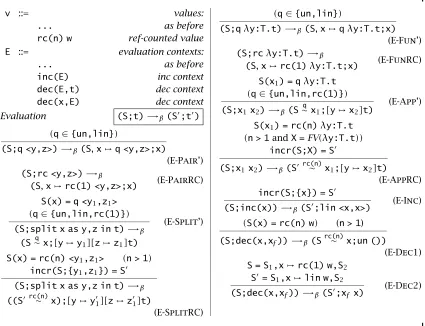
In order to define the execution behavior of reference-counted data struc-tures, we will define a new sort of stored value with the formrc(n) w. The integern is the reference count: it keeps track of the number of times the value is referenced elsewhere in the store or in the program.
different sorts of uses. Second, we extend the notation S∼qx so that q may be rc(n) as well aslin andun. If nis 1 then Src(n)∼ x removes the binding x,rc(n) wfromS. Otherwise,Src(n)∼ xreplaces the bindingx,rc(n) wwith x,rc(n-1) w. Finally, given a storeSand a set of variablesX, we define the function incr(S;X), which produces a new store S0 in which the reference count associated with any reference-counted variablesx∈Xis increased by 1. To understand how the reference counting operational semantics works, we will focus on the rules for pairs. Allocation and use of linear and unre-stricted pairs stays unchanged from before as in rules(E-Pair’)and(E-Split’). Rule(E-PairRC) specifies that allocation of reference-counted pairs is simi-lar to allocation of other data, except for the fact that the dynamic reference count must be initialized to 1. Use of reference-counted pairs is identical to use of other kinds of pairs when the reference count is 1: We remove the pair from the store via the function Src(n)∼ x as shown in rule and substi-tute the two components of the pair in the body of the term as shown in (E-Split’). When the reference count is greater than 1, rule(E-SplitRC)shows there are additional complications. More precisely, if one of the components of the pair, say y1, is reference-counted then y1’s reference count must be
increased by 1 since an additional copy ofy1is substituted through the body
oft. We use theincr function to handle the possible increase. In most re-spects, the operational rules for reference-counted functions follow the same principles as reference-counted pairs. Increment and decrement operations are also relatively straightforward.
In order to state and prove the progress and preservation lemmas for our reference-counting language, we must generalize the type system slightly. In particular, our typing contexts must be able specify the fact that a particular reference should appear exactlyntimes in the store or current computation. Reference-counted values in the store are described by these contexts and the context-splitting relation is generalized appropriately. Figure 1-18 sum-marizes the additional typing rules.
1.3.7 Exercise [«««,3]: State and prove progress and preservation lemmas for the simply-typed linear lambda calculus (functions and pairs) with reference
counting. 2
1.4
An Ordered Type System
1.4 An Ordered Type System 31
v ::= values:
... as before
rc(n) w ref-counted value
E ::= evaluation contexts:
... as before
inc(E) inc context
dec(E,t) dec context
dec(x,E) dec context
Evaluation (S;t) -→β(S0;t0)
(q∈{un,lin})
(S;q <y,z>) -→β(S,x,q <y,z>;x)
(E-Pair’) (S;rc <y,z>) -→β
(S,x,rc(1) <y,z>;x) (E-PairRC)
S(x) = q <y1,z1> (q∈{un,lin,rc(1)})
(S;split x as y,z in t) -→β
(S∼q x;[y,y1][z,z1]t)
(E-Split’)
S(x) = rc(n) <y1,z1> (n > 1)
incr(S;{y1,z1}) = S0
(S;split x as y,z in t) -→β
((S0rc(n)∼ x);[y,y0
1][z,z01]t)
(E-SplitRC)
(q∈{un,lin})
(S;qλy:T.t) -→β(S,x,qλy:T.t;x)
(E-Fun’) (S;rcλy:T.t) -→β
(S,x,rc(1)λy:T.t;x) (E-FunRC)
S(x1) = qλy:T.t (q∈{un,lin,rc(1)})
(S;x1x2) -→β(S∼q x1;[y,x2]t)
(E-App’)
S(x1) = rc(n)λy:T.t (n > 1andX =FV(λy:T.t))
incr(S;X) = S0
(S;x1x2) -→β(S0rc(n)∼ x1;[y,x2]t)
(E-AppRC) incr(S;{x}) = S0
(S;inc(x)) -→β(S0;lin <x,x>)
(E-Inc)
(S(x) = rc(n) w) (n > 1)
(S;dec(x,xf)) -→β(Src(n)∼ x;un ())
(E-Dec1) S = S1,x,rc(1) w,S2
S0= S1,x,lin w,S2
(S;dec(x,xf)) -→β(S0;xf x)
[image:46.576.80.505.73.399.2](E-Dec2)
Figure 1-17: Linear lambda calculus: Reference counting operational semantics
exchange property, we are able to guarantee that certain values, those values allocated on the stack, are used in a first-in/last-out order.
Syntax
Γ ::= typing contexts:
... as before
Γ,x:rc(n)P rc(n) context
Store Typing
`S:Γ1◦Γ2 Γ1`rc w:rc P `S,x,rc(n) w:Γ2,x:rc(n) P
(T-NextrcS)
Context Splitting
Γ=Γ1◦Γ2 n = i + j Γ,x:rc(n)P=
(Γ1,x:rc(i)P)◦(Γ2,x:rc(j)P)
(M-RC)
(wheniorjis 0, the corresponding binding is removed from the context)
Variable Typing
un(Γ1,Γ2)
Γ1,x:rc(1)P,Γ2`x:rc P
(T-RCVar)
Figure 1-18: Linear lambda calculus: Reference counting run-time typing
Syntax
The overall structure and mechanics of the ordered type system are very similar to the linear type system developed in previous sections. Figure 1-19 presents the syntax. One key change from our linear type system is that we have introduced an explicit sequencing operationlet x = t1in t2 that first
evaluates the termt1, binds the result tox, and then continues with the
eval-uation oft2. This sequencing construct gives programmers explicit control
over the order of evaluation of terms, which is crucial now that we are intro-ducing data that must be used in a particular order. Terms that normally can contain multiple nested subexpressions such as pair introduction and func-tion applicafunc-tion are syntactically restricted so that their primary subterms are variables and the order of evaluation is clear.
The other main addition is a new qualifierordthat marks data allocated on the stack. We only allow pairs and values with base type to be stack-allocated; functions are allocated on the unordered heap. Therefore, we declare types ord T1→T2and termsordλx:T.tto be syntactically ill-formed.
Ordered assumptions are tracked in the type checking contextΓlike other assumptions. However, they are not subject to the exchange property. More-over, the order that they appear in Γ mirrors the order that they appear on the stack, with the rightmost position representing the stack’s top.
Typing