Abstract: Real time location/unknown target position is important in Electronic Warfare (EW) system. To find the location the hyperbolic multilateration method is used. Many algorithms are available to solve nonlinear hyperbolic equations. The techniques which are mostly used for solving and determining non-linear measurements are the Taylor Series method and Ezzat’s approach. Taylor series approach computes the position fix in an iterative fashion where as Ezzat’s solution gives a direct solution. In this paper to solve the non-linear measurements which are in the hyperbolic form we used two types of techniques. These two techniques are implemented on different receiver/ sensors distributions ex. square, triangle etc. In this paper we explores the optimal value for different receiver combinations and also we compares the convergence issues, relative performance for all combinations and in three dimensions. Finally we determined the standard deviation for every case and compared it for better optimal solution.
Index Terms: multilateration, Optimal distribution, Receivers, TDOA.
I. INTRODUCTION
Emitter Location finding enables important functionality for both military and civilian applications. Military forces targeted on enemies locations to save their countries. For precise and unambiguous of any moving objects or targets in warfare’s the major focus is on the electromagnetic [1] [2]. It is important to know to determine the position in warfare. There are two types of location determination (LD) types are namely active, passive and these techniques are used for decades. For ex. radars location determination is based on active LD technique [3-4]. When active location finding techniques uses detectable RF signals so the enemy knows that they are being tracked or located [3] [4]. Passive location determination (PLD) the enemy does not know that they have been tracked or targeted or located this is the advantage in PLD. Many engineers and scientists have developed this passive location determination technique with the great efforts. These techniques are based on enemies electromagnetic spectrum interception, rather than emanating friendly EM transmissions. To locate moving objects/targets, in motion many location techniques are employed. Source localization can be based on arrival of signal based on time (TOA), based on angle (AOA), difference of arrival based on time called time difference of arrivals (TDOA) or combination of them.
Revised Manuscript Received on September 06, 2019
P Balakrishna, Dept of ECE, Vignan’s Nirula Inst of Tech and Sci for women, Guntur, India.
M Divya Sree, Dept of ECE, Vignan’s Nirula Inst of Tech and Sci for women, Guntur, India.
SD Nageena Parveen, Research Scholar, Department of ECE, Acharya Nagarjuna University, Guntur, India.
When the Emitter and receiver are moving or one of them is moving so the frequency difference of arrivals (FDOA) can be exploited to improve location accuracy [5].
The Common techniques used for finding unknown target position are Difference of Arrival based on time called as Time Difference Of Arrival (TDOA), TOA (Time of Arrival), AOA (Angle of Arrival) and FDOA (Frequency Difference of Arrival). In present scenario, TDOA techniques are most widely used location determination technique using hyperbolic multilateration. It involves fixing of target the set of sensors have to be arranged in predetermined positions [6]. Taylor Series and Ezzat’s algorithms are used to perform hyperbolic multilateration solutions [4]. In this paper, discuss the convergence issue of the method with respect to predetermined target is given.
This paper is explained in IV sections. In section II introduces TDOA measurement and the method of two algorithms. The section III deals with the distribution of sensors. Section IV the given method convergence and if the receiver geometry changes how it effects on convergence of method is given, comparison of methods biases in measurement, for better accuracy selecting the best distribution of sensor, and finally the paper concluded in section V.
II. HYPERBOLICMULTILATERATION(TDOA)
METHOD
To find the position in hyper multiletaration the method is divided in to two stages. In the first stage the determination of difference of arrival in ranges [8]. To determine the RDOA the method must use the estimated time delay. RDOA is determined time difference of arrival multiplied by speed of light. Here let us take the estimation of the location unknown target be (xt, yt, zt).there are three unknown in three dimensions to solve this three unknowns minimum required non-liner equations are three. The unknown target is determined with necessitating the availability of a minimum of four receivers [9]. The four sensors are placed at a locations called l, s, n and 0 has been taken as
(
x
l,
y
l,
z
l)
,) , , ( ), , , ( ), , ,
(xs ys zs xn yn zn xo yo zo respectively the distances can
be calculated as given below:-
) 1 ( )
( ) ( ) (
) ( ) ( ) (
) ( ) ( ) (
) ( ) ( ) (
2 2
2
2 2
2
2 2
2
2 2
2
t o t o t o o o
t n t n t n n n
t s t s t s is s
t l t l t l l l
z z y y x x ct d
z z y y x x ct d
z z y y x x ct d
z z y y x x ct d
In eq. 1 the range of arrival is given the difference of arrival in range can be calculated as
above:-
Unknown Location Determination using TDOA
Computation with Convergence Points
) 2 ( )
( ) ( ) (
) ( ) ( ) (
2 2 2 2 2 2
2 1 2 1 2 1
2 1 1 2
t t
t
t t
t
z z y y x x
z z y y x x
d d d
Where
(1,2){(l,s),(l,n),(l,o),(s,n),(s,o),(n,o)}.
Each equation represents the hyperbolic curve and the intersection of these hyperboloids gives the exact position of the unknown target.
Fig.1 Hyperboloid with its two foci
The major focus is on the multileration by hyperboloids [10]-[12]. In eq. (2) the difference of two ranges of arrival gives the less biases because of the elimination of receiver common errors due to channel. This is the advantage of multileration using time difference of arrival.
III. METHODOFIMPLEMENTATION A. Taylor Series
The hyperbolic position of target estimation has to be accurate and precise to position location problem. There are various algorithms available [13]. One of the direct method to solve linear equations are Ezzat’s series. But the method involves intensive mathematical computations and becomes complex as the number of receivers increases.
In this paper two methods are taken and compared, direct method (Ezzat’s method) and Taylor’s series. Another popular method is Taylor algorithm. It is an iterative loop algorithm which continuously reduces the error as minimum as possible and gives the best optimal solution to the given problem [14].
Following are the steps given for Taylor’s series algorithm. Determining the ROA values. There by finding RDOA values. eq. (3), eq. (4) here the higher order terms have neglected only first order terms are
TDOA=c(dk-d1)
) 3 ( )
( ) ( ) (
) ( ) ( ) (
2 1 2 1 2 1
2 2
2 1 1
t t
t
t l t l t l
l l
z z y y x x
z z y y x x
d d d
Expanding the equation (3) using Taylor series and retaining the 1st two terms gives
) 4 ( 3
2 1 1
1 vs s x s y s z
i d a a a
d
)
)
(
)
(
)
(
)
(
)
(
)
(
(
2 1 2
1 2
1
2 2
2 1
z
z
y
y
x
x
z
z
y
y
x
x
C
d
v v
v
s v s v s
v vs
Where
) , ,
(xv yv zv is the initial guess used in the calculation.
) , ,
(x y z Are the incremental values of(xt,yt,zt)obtained at
the end of each successive iteration.
1 1 1
3
1 1 1
2
1 1 1
1
d z z d
z z x d a
d y y d
y y x d a
d x x d
x x x d a
i i i i
i i i i
i i i i
The nonlinear equations can be linearized as
)
5
(
A
Where,
n c n b n a
b c b b b a
a c a b a a
vn l n l
l v l
l v l
a a a
a a a
a a a
d d
d d
d d
A
. . .
. . .
.. .. .. ..
2 2
1 1
incremental values of (x,y,z)and can be obtained by using
) 6 ( )
( 1 A
T
T
The iterative loop will be ended with zero error and target location is updated as
z v t y v t x v
t x y y z z
x , ,
B. Ezzat’s Method
The unique solution is obtained by Ezzat’s and it is a direct solution approach. This approach does not depend upon range ROA values [15]. It takes direct of TDOA measurement to find the target location, where as in Taylor’s series approach the TDOA measurements are obtained by range data. In closed form solution the measurement does not depends on range. In this method it does not require any other information rather than time ta [16]. This is the only technique that can be used without the range data i.e. without ta, it is possible to find the location of the emitter [17]. The closed-form solution presented here does not depend on the availability of any information other than The Times of arrival. The basic form of time of arrival equation is as follows
Let us take ta
) 7 (
c D t ti a j
Where ti arrival of the signal depends on time, Dj distance between sensor and target, c velocity of light as signal travels in air/vacuum, ta unknown if we take more than two sensors the ta value will be cancelled.
) 8 (
1 2 1 2
c D D t
t
This is the TDOA equation. This equation yields a 3D hyperboloid as mentioned before. When the emitter coordinates
(
X
b,
Y
b,
Z
b)
and are plugged into this equation (8) can be written as) 9 ( ) ( ) ( ) ( ) ( ) ( ) ( ) ( 2 2 2 2 2 2 i j b j b j b j b i b i b i t t C Z Z Y Y X X Z Z Y Y X X
Therefore this equation represents a time difference of arrival. Where
(
X
i,
Y
i,
Z
i)
and(
X
j,
Y
j,
Z
j)
are the predefined positions of the sensors and having three more receiving antennas yields. Let us take emitter location be at. 0 0 0, , ) (X Y Z
For more than 2 receivers, we get more number of non-linear equations if solve the non-linear equations then we get the estimated target position. In case of signal path is non-linear and signal propagated through a medium with velocity less than velocity of light in such a case the equations are
) 10 ( 1 ) ( i i j j i i j j i j D D c c D c D t t
Where αj, αi are delay coefficients of the path which are less than (or) equal to one in this case we have assumed that there is no path delay so αj=αi=1.
The vector format of hyperbolic equations
) 11 ( 0 P P
di i
Where Pi(Xi,Yi,Zi) is the vector of position for the antenna, )
, ,
( 0 0 0
0 X Y Z
P is the vector of the position of target.
Equation (11) represents the difference between the two vectors. We modify Equation (11)
) 12 ( 1 ) ( ) ( 2 1 2 1 2 2 2 2 2 2 0 1 2 0 2 D D c t t t t
From eq.11 and eq.12 we have
) 13 ( ) 2 2 ( 1 2 0 2 1 0 2 2 0 2 2 2 2 1 2 0 1 2 2 2 0 2 t t t t t t t t c P P P P Where ) 14 ( 2 0 2 0 2 2
0 P P P P
P
P T
i i
i
T i
P is the transpose of vectorPi .
substitute Equation (14) into Equation (13)
) 15 ( ) ( 2 ) ( 2 ) ( 2 ) ( 2 2 1 2 2 0 2 1 2 2 2 2 1 1 2 2 2 0 2 1 2 1 2 2 2 2 1 2 2 0 2 1 2 2 2 2 1 0 1 2 0 2 1 2 2 0 2 2 0 2 2 t t c t t t c P P P P P t t c t t t c P P P P P P P P T T T T
In Equation (15) there are two unknownst0 and
0
P . To solve these unknowns the different sensors combinations are consider.
five receivers to work [23].
Equation (15) is divided by TDOA, then
) 16 ( 2 ) ( ) ( 2 ) ( 1 2 0 1 2 2 2 1 1 2 2 2 1 2 0 2 1 2 1 2 2 2 2 1 2 c t t t c P P t t P P P t t T T
By similarly sensors combinations 3-1 and 4-1
) 17 ( 2 ) ( ) ( 2 ) ( 1 2 0 1 3 2 2 1 1 2 3 3 1 3 0 2 1 2 1 2 3 2 3 1 3 c t t t c P P t t P P P t t T T ) 18 ( 2 ) ( ) ( 2 ) ( 1 2 0 1 4 2 2 1 1 2 4 4 1 4 0 2 1 2 1 2 4 2 4 1 4 c t t t c P P t t P P P t t T T
The next step is to eliminatet0 from Equations (16), (17) and
(18). Equations (15) and (17) are merged in the components of P0 to get rid of t0. This result in
) 19 ( 2 2 ) ( ) ( 1 ) ( 1 2 1 1 2 3 3 1 3 2 1 1 2 2 2 1 2 0 2 3 2 2 1 2 1 2 3 2 3 1 3 2 1 2 1 2 2 2 2 1 2 T T T
T P P
t t P P t t P t t c P P t t P P t t
Similarly Equations (16) and (17) yield
) 20 ( 2 2 ) ( ) ( 1 ) ( 1 2 1 1 2 4 4 1 4 2 1 1 2 2 2 1 2 0 2 4 2 2 1 2 1 2 4 2 4 1 4 2 1 2 1 2 2 2 2 1 2 T T T T P P t t P P t t P t t c P P t t P P t t
Because of unknown terms we additionally add another sensor to find additional unknowns and for sensors combination 5-1. ) 21 ( 2 2 ) ( ) ( 1 ) ( 1 2 1 1 2 5 5 1 5 2 1 1 2 2 2 1 2 0 2 5 2 2 1 2 1 2 5 2 5 1 5 2 1 2 1 2 2 2 2 1 2 T T T T P P t t P P t t P t t c P P t t P P t t
2
1 2 1 2 1 2 1 2 5
2 5 2 5 2 5 1 5 2 1
2 1 2 1 2 1 2 2
2 2 2 2 2 2 1 2 1
) (
1 )
( 1
Z Y X Z Y X t t Z Y X Z Y X t t b
The remaining unknowns can be determined from equations (20) and (21). Equation (22) can be expressed as
B AX
Linearized format of the estimation is
B A A A
X T T
* ) *
( 1
IV. WORKINGMETHODOLOGYAND
OBSERVATIONSREGARDINGTHEISSUE
OFCONVERGENCE
Step 1:- the following method is used and given in step wise Step 2:- choose target let us take this case we chosen a target as 7km,12km,0.2km)
Step 3:-in Taylor series the estimation is depends on initial co-ordinates of the target here let take (2km, 2km, 0.5km) Step 4:-fix the base sensor at some point and measurement are w.r.t to sensor 1 to other sensors differences of arrival in time. Here 5 sensors are taken 1 is fixed and other sensors are any possible combination.
I.Receiver Distributions Base sensor =0km, 0km, 0.05km.
Here added noise is Gaussian with a standard deviation of 10-8 and 10-9 is given. In case 1, 10-8 Gaussian is added as we observe from the table for different sensors distributions the different target positions are obtained. The target is then estimated for all the configurations and related observations are made. The same process is now repeated for reduced noise values i.e. Gaussian noise with a standard deviation of 10-9 is now added to the TDOA values and the resultant observations are noted.
II.Estimated target for different sensors distributions. Sensors geometry
Location Co-ordinates (in m)
Sensor 1 Sensor 2 Sensor 3 Sensor 4
Square (2000, 0, 0) (0, 2000, 0) (-2000, 0, 0) (0, -2000, 0) Trapezoidal (w/out
altitude difference)
(-2000, 0, 50)
(-1000, 2000, 50)
(1000, 250, 0.05)
(2000, 0, 50)
Trapezoidal (with altitude difference)
(-2000, 0, 100)
(-1000, 2000, 150)
(1000, 250, 200)
(2000, 0, 25) Straight Line (w/out
altitude difference) (-2000, -2000, 99)
(-1000, 0, 100)
(0, 2000, 100) (1000, 4000, 100) Straight Line (with
altitude difference) (-2000, -2000, 25)
(-1000, 0, 100)
(0, 2000, 150) (1000, 4000, 200) Parallelogram (-1000, 0,
20)
(-2000, -2000, 200)
(0, 2000, 200) (-3000, 0, 200) III. Estimated target positions with standard deviations
10-8 and 10-9
A.Ezzat’s Approach:
This is direct position finding technique. This paper does not cover the effects like multipath. Here the path delay is neglected.
i). The Arrivals based on range is determined with the predefined estimated target.
ii). The ROA are input for the program code. Therefore the errors are introduced. From this MATLAB code and all alphas are considered as one.
ii). Since biases are added in TOA measurements by adding Gaussian noise to work with real time data. Two cases considered similar to Taylor algorithm, no need of any initial guess.
iii). Simulation has been performed in MATLAB. The Observations from Table IV and V as follows:
i) When the Gaussian error with std 10-9 is added the better results are obtained.
ii) Sometimes the algorithm convergence and not convergent depends on different altitude, added Gaussian. iii) When the receivers are arranged on a straight line with variations in altitude, the algorithm converges when noise the close value of the estimated target is obtained.
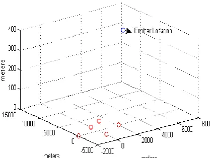
iv) The sensors are placed in three different arrangements like wide arrangement, closed spaced and randomly spaced. The Target estimation by using different geometric configurations are shown in Fig. 2, Fig. 3 and Fig. 4. Distribution
of Receivers
Estimated Target Location (in m) Taylor’s series
approach
Ezzart’s approach
Square (7021.3,12037, 233.6662)
(7987.7,12983,349.5)
Trapezoidal(w/out altitude difference)
(6984.5,11976,125.921 9) with initial z = 300
Not convergent (NC)
Trapezoidal(with altitude difference)
(7001.0, 11999,213.7736)
(7987.7,12983,408.08)
Straight line (with out altitude difference)
(6982.6,11976, 164.4529) with initial z = 300
Result’s may be in accurate
(8127.1,13015,2224.6) Straight Line (with
altitude difference)
(6961, 11939, 211.3699)
Result’s may be in accurate
(11614,9496.1,71927) with Z=300
Parallelogram (7323.4, 12418,596.5420)
(7997.3,12999,290.60)
Lozenge (7012.7,
12020,196.9786)
(8179.04,13305.06,396.6 7)
Inverted Triangle (6956.6, 11941,170.6866)
(8071.2,13102,358.79) with initial z = 100
Distribution of Receivers
Estimated Target Location (in m)
Noise with stddev = 10-8 added
Noise with stddev = 10-9
added
Square (7087.8, 12121, 622.21)
(7021.3, 12037, 233.6662)
Trapezoidal (w/out altitude difference)
Not convergent (NC) (6984.5, 11976, 125.9219) with initial z = 300
Trapezoidal (with altitude difference)
(7037.3, 12010, 260.71)
(7001.0, 11999, 213.7736)
Straight line (with out altitude difference)
NC (6982.6, 12000, 164.4529)
Straight Line (with altitude difference)
(9129.4, 15351, 1168.9)
(6961, 11939, 211.3699)
Parallelogram Convergent with negative altitude
(7323.4, 12418, 596.5420)
Lozenge (7459, 12715, 196.5741)
(7012.7, 12020, 196.9786)
Inverted Triangle (7258.3, 12378, 612.2787) with initial z = 300
IV. Target location estimates for various receiver distribution, noise with std dev = 10-8 and 10-9added
V. Target deviation
Sensors distribution Taylor series
St.line (w/o) 1.2389*10^2
St.line with altitude difference 731.7646 Trapezoidal(with altitude difference) 3.5733
Parallelogram 1.33*10^2
Lozenge 133
Inverted triangle 422
In table V, sensor’s distribution comparisons of deviation in target location. The standard deviation is less in trapezoidal with altitude difference.
V.CONCLUSIONS
[image:5.595.308.546.55.231.2]In this paper, we explains the hyperbolic multilateration approach to obtain the position of a target which is unknown. The main concentration of this paper is finding unknown target with taylor series approach and drawn some conclusion on its convergence. This praposed method is easy to evaluate the position. That the convergence of the proposed method is relying on the type receiver configuration such as square, traingle etc. One important observation that can act as a basis for further study is the better convergence observed with variation in the receiver altitudes when compared to the case where the receivers are located at the same altitudinal level. However, the dependence of convergence of the algorithm on the relation between the initial guess and the receiver location needs to be explored further.
Fig.2 Target Estimation with Square Distribution of Sensors
[image:5.595.319.540.275.442.2]Fig.3 Target Estimation with Straight Line Distribution of Sensors
Fig. 4 Target Estimation with Lozenge Distribution of Sensors
REFERENCES
1. R. Stansfield, “Statistical theory of DF fixing,” Journal of IEE, vol. 94,no. 15, pp. 762–770, 1947.
2. M. Schmidt, “A new approach to geometry of range difference location ,”IEEE Trans. Aerospace and Electronic Systems, vol. 8, no. 6, pp. 821–835, November 1972.
3. K. Ho and Y. Chan, “Solution and performance analysis of geolocation by TDOA,” IEEE Trans. Aerospace and Electronic Systems, vol. 29, no. 4,pp. 1311–1322, October 1993.
4. N. Okello and D. Musicki, “Measurement association and tracking for emitter localisation using paired UAVs ,” Journal of Advances in Information Fusion (submitted).
5. R. Bardelli, D. Haworth, and N. Smith, “Interference localisation for the Eutelsat satellite system,” in Global Telecommunications Conference, GLOBECOM ’95, vol. 3, Singapore, November 1995, pp. 1641–1651.
6. P. Chestnut, “Emitter location accuracy using TDOA and differential Doppler,” IEEE Trans. Aerospace and Electronic Systems, vol. 18, no. 2,pp. 214–218, March 1982.
7. Aatique , M. (1997) Evaluation of TDOA techniques for position location in CDMA systems. (Master's thesis, Virginia Polytechnic Institute and State University) , 15–23.
8. Adamy, D. L. (2004). Accuracy of emitter location systems. EW-102: A second course in electronic warfare (pp. 155–187). Boston: Artech House.
9. Bard, J. D, & Ham, F. M. (1999) . Time difference of arrival dilution of precision and applications. IEEE Transactions on Signal Processing, 47(2), 521–523. doi:
10.1109/78.740135 Distribution
of Receivers
Estimated Target Location (in m)
Taylor’s series approach Ezzart’s approach
Square (7021.3,12037, 233.6662) (7987.7,12983,349.5)
Trapezoidal(w/out altitude difference)
(6984.5,11976,125.9219) with initial z = 300
Not convergent (NC)
Trapezoidal(with altitude difference)
(7001.0, 11999,213.7736) (7987.7,12983,408.08)
Straight Line (w/out altitude difference)
(6982.6,11976, 164.4529) with initial z = 300
Result’s may be in accurate (8127.1,13015,2224.6)
Straight Line (with altitude difference)
(6961, 11939, 211.3699) Result’s may be in accurate (11614,9496.1,71927) with Z=300
Parallelogram (7323.4, 12418,596.5420) (7997.3,12999,290.60)
Lozenge (7012.7, 12020,196.9786) (8179.04,13305.06,396.67)
[image:5.595.63.272.603.760.2]10. Chan, Y. T., & Ho , K. C. (1994). A simple and efficient estimator for hyperbolic location . IEEE Transactions on Signal Processing, 42(8), 1905–1915. doi: 10.1109/78.301830
11. Chan, Y. T., & Ho , K. C. (2003). TDOA-SDOA estimation with moving source and receivers . 2003 IEEE International Conference; Acoustics, Speech , and Signal Processing, (ICASSP '03). , 5 V-153-6. doi: 10.1109/ICASSP.2003.1199891
12. Ezzat, G. B. (2006). Closed-form solution of hyperbolic geolocation equations. IEEE Transactions on
13. C.Knapp, & G. Carter, (1976) . The generalized correlation method for estimation of time delay. IEEE Transactions on Acoustics, Speech and
Signal Processing, 24(4), 320–327. doi:
10.1109/TASSP.1976.1162830
14. D.Musicki, &W. Koch, (2008) . Geolocation using TDOA and FDOA measurements. 11th International Conference on Information Fusion , Cologne. 1–8.
15. Poisel, R. (2002). Direction-finding position-fixing techniques, hyperbolic position-fixing techniques . Introduction to communication electronic warfare systems (pp. 331–424) . Boston: Artech House. 16. Sathyan . T,. Kirubarajan.T, & Sinha, A. (2004). Geolocation of
multiple emitters in the presence of clutter . Signal Processing, Sensor Fusion, and Target Recognition XIII, Proceedings of the SPIE, 5429, 66–76. doi: 10.1117/12.542259
17. Ho, K. C., & Chan, Y. T. (1993). Solution and performance analysis of geolocation by TDOA. IEEE Transactions on Aerospace and Electronic Systems, 29(4), 1311–1322. doi: doi:10.1109/7.259534 18. Loomis, H. H. (2007). Geolocation of electromagnetic emitters.
(Technical Report No. NPS-EC-00-003). Monterey, CA, USA: Naval Postgraduate School.
19. Xu, J., Ma, M., & Law, C. L. (2006). Position estimation using UWB TDOA measurements. Ultra-Wideband, the 2006 IEEE 2006 International Conference on, 605–610.
20. Yan-Ping Lei, Feng-Xun Gong, & Yan-Qiu Ma. (2010). Optimal distribution for four-station TDOA location system. Biomedical Engineering and Informatics (BMEI), 2010 3rd International Conference on, 7 2858–2862.
21. Torrieri, D. J. (1984). Statistical theory of passive location systems. Aerospace and Electronic Systems, IEEE Transactions on, AES-20(2), 183–198. doi: 10.1109/TAES.1984.310439
22. Vaccaro, D. D. (1993). Passive direction finding and geolocation. Electronic warfare receiving systems (pp. 221-253). Boston: Artech House.
23. Chan, Y. T., & Ho , K. C. (2003). TDOA-SDOA estimation with moving source and receivers. 2003 IEEE International Conference; Acoustics, Speech, and Signal Processing, (ICASSP '03), 5 V-153-6. doi: 10.1109/ICASSP.2003.1199891
24. Lipsky, S. E. (1987). Interferometer DF techniques. Microwave passive direction finding (pp. 155–171). Newyork: John Wiley & Sons.
AUTHORSPROFILE
P Balakrishna obtained a B.Tech degree in Electronics and Communication Engineering from SASTHARA institute of technology, 2008. He received her M.Tech degree from GRIET, Hyderabad. He is doing his Ph.D. program in the Annamalai University, Tamil Nadu, India. Presently he was working as Assistant professor in Vignan’s Nirula Inst. Of Technology and Science for women, India.
M Divya Sree obtained a B.Tech degree in Electronics and Communication Engineering from Chirala engineering college, 2009. She received her M.Tech degree from Vignan’s University, 2011. Presently she was working as Assistant professor in Vignan’s Nirula Inst. Of Technology and Science for women, India.
SD. Nageena Parveen obtained a B.Tech degree in Electronics and Communication Engineering from SCR College of engineering in 2010. She received her M.Tech degree from Andhra University Visakhapatnam. She is doing her Ph.D. program in the ANU College of Engineering and Technology, Acharya Nagarjuna University, Guntur, India.