International Journal of Innovative Technology and Exploring Engineering (IJITEE) ISSN: 2278-3075,Volume-8 Issue-12, October 2019
Abstract: The building sector consumes more than 25% of energy consumption in Morocco. So, the reducing of the energy cost of building has become a necessity. In this context, the objectives of this work are to investigate the thermophysical properties and the energy performance of earthen walls made from three types of unfired clay bricks. This work is broken into two steps. In the first step the apparent thermal conductivity was obtained experimentally using the hot plate method. In the second step, the thermophysical properties obtained were used to calculate the decrement factor and the time lag of complete walls mad from these materials by solving the transient heat conduction equation with periodic loadings using the eigenfunction expansion and the integrating factor methods. The effect of the outer and inner combined convection and radiation heat transfer coefficient on these dynamic thermal characteristics was studied. The optimum thickness of the walls was also calculated. Finally, the effect of thermal insulation on energy performance of the walls was studied
Keywords : Energy performance, Thermal inertia, Analytical solution, Numerical solution, Earthen walls.
I. INTRODUCTION
In Morocco about 95% of energy needs are imported. This is why the national energy strategy is based on the promotion of renewable energies and energy efficiency, particularly in the building sector. Indeed, if the latter is one of the largest consumers of energy, it also has great savings potential thanks to the rational management of technical equipment, the thermal optimization of the walls, etc. The recent Construction Thermal Regulation in Morocco (RTCM) is timely. Designed for new buildings, its objective is to ensure a certain thermal comfort while being more energy efficient according to thermal and energy specifications of the envelope and equipment.. Despite the disadvantages of earth constructions (maintenance, deterioration ...), they can be made sustainable and renewable if they are properly maintained, thus offering certain advantages such as reducing the impact on the environment and energy consumption. [1]-[2]-[3]-[4].
The works [21]-[22]-[17] have focused on the evaluation of thermal properties and have highlighted the thermal performance of composite materials based on earth and fibers but their dynamic thermal characteristics have not studied.
Revised Manuscript Received on October 05, 2019.
Yassine Chihab*, Mohammed V University in Rabat, Materials, Energy and Acoustics TEAM, Morocco.
Email: [email protected]
Mohammed Garoum, Mohammed V University in Rabat, Materials, Energy and Acoustics TEAM, Morocco
Najma Laaroussi, Mohammed V University in Rabat, Materials, Energy and Acoustics TEAM, Morocco
In the following, we present a series of research studies have been done concerning the dynamic thermal performances of building walls such as the work of El Fgaier et al [5] which investigated thermal capacity, time lag and the decrement factor using the NF EN ISO 13786 standard. It should be noted that the thickness affect significantly these thermal inertia quantity. Another work of El Fgaier et al [6] studied the dynamic thermal performance of demonstrative earthen construction in real conditions. Ozel[7] analyzed numerically the time lag and the decrement factor for composite wall. Economical and environmental impact of the insulating layer thickness was studied.
Asan et al. [8] also investigated numerically the time lag and the decrement factor by solving one-dimensional transient heat conduction equation using Crank-Nicolson scheme. In this study the effect of thickness and the type of material were evaluated. In Ozel[9]optimum insulation thickness according to cooling requirements of buildings in a hot climate was investigated numerically. Al-Sanea and Zedan [10] investigated the decrement factor of two wall configurations using single layers of thermal mass and thermal insulation. Ulgen et al [11] analyzed the thermal behavior of walls of opaque buildings exposed to solar radiation. They calculated the time lag and the decrement factor using experimental and theoretical methods. They also examined the effect of thermophysical properties on the energy performance of the walls studied. Also, Asan et al. [12]investigated numerically the effect of wall’s insulation thickness and their position on time lag and decrement factor. Önder Kaskaet al. [13] conducted an experimental and a numerical investigation to determine time lag, decrement factor and total equivalent temperature difference values for multilayer walls and flat roofs of buildings in Turkey.
The majority of works the time lag and the decrement factor are investigated numerically. In this investigation, the dynamic thermal characteristics of multilayer walls are determined analytically by solving the transient heat conduction equation with periodic loadings using the eigenfunction expansion combined with the integrating factor methods.
II. THERMALCONDUCTIVITYESTIMATIONBY
THESTATEHOTPLATEMETHOD
The method of the stationary hot plate permits to estimate the thermal conductivity at the steady state .
Energy Performance of Earthen Walls In A Hot
Climate of Morocco
Its schematic principle is described in the Figure 1
This method is based on temperature measurements at the center of heating element inserted between the sample and an insulating polyethylene foam layer. The heating element is a flat and thin electrical resistance .The power dissipated by joule effect is known and the flux is considered uniform over its entire surface of the sample. Once the system reaches the steady state regime and assuming one-dimensional heat conduction, we can write:
2
1 2
U
R.S
(1)
1
1 0 1
1
T
T
e
(2)
2
2 0 2
2
T
T
e
(3)
1
2
2 0 2
0 2 2
e
T
T
T
T
e
(4)
ø is the total heat flow emitted by the heating element. λ1
The thermal conductivity of the sample, e1 the thickness of the sample; λ2= 0.047 W.m-1.K-1and e2 = 10 mm: are
[image:2.595.284.548.98.363.2]respectively thermal conductivity and thickness of the insulating foam.
Fig. 1.Schema of hot plate in steady state regime
III. DYNAMICTHERMALCHARACTERIZATION
OFTHEWALLWITHSINUSOIDALLOADINGS
A. Mathematical model
This section is dedicated to the Analytical study of the thermal dynamic response of a wall located in city of Marrakech and composed of materials studied in the first section.
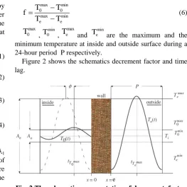
The time lag and decrement factor describe the dynamic thermal behavior of a building component when subjected to time-dependent conditions limits. The decrement factor is an indication of the external thermal load penetration, and is defined as the ratio of internal thermal temperature peak to external thermal temperature peak. The time lag indicates how long exterior temperature changes take to affect interior conditions.
The time lag is defined as:
max max max max
0 e 0 e
max max max max
0 e 0 e
max max
0 e
t T
t T
t T
t T
.
t T
t T
t T
t T
P.
t T
t T
P.
(5)
Where
max 0
t T
and
max e
t T
,(h) represent the time in
hours when inside and outside surface temperatures are at their maximums, respectively, and P (24 h) is the period of the wave.
While the decrement factor is defined as:
max min
0 0
max min
e e
T
T
f
T
T
(6)max 0
T
, min 0T ,
T
emax and mine
T are the maximum and the
minimum temperature at inside and outside surface during a 24-hour period P respectively.
Figure 2 shows the schematics decrement factor and time lag.
Fig. 2.The schematic representation of decrement factor
and time lag
If we assume one-dimensional transient heat conduction through an opaque finite length wall without any heat sources, the temperature in the wall is governed by the following equation :
2
2
T x, t
1
T x, t
.
a
t
x
(7)Two boundary conditions on both sides of wall and one initial condition are needed to solve this equation:
At the inner surface
x 0 1 1 i
T x, t
.
h .T 0, t
h .T .
x
(8) While at the outer surface
x e 2 2 s a
T x, t
.
h .T e, t
h T
t
x
(9)These two boundary conditions are nonhomogeneous time-dependent third kind’s
[image:2.595.55.282.370.464.2]International Journal of Innovative Technology and Exploring Engineering (IJITEE) ISSN: 2278-3075,Volume-8 Issue-12, October 2019
max min max mins a min
T T 2 t T T
T t Sin T
2 P 2 2
(10)
According to the temperature variation of the city of Marrakech during a 24-hour period of day on 15 August 2019 [14].Sol air temperature is given by the following equation:
max min max mins a min
T T 2 t T T
T t Sin T
2 P 2 2
40 24 2 t 40 24
Sin 24
2 86400 2 2
2 t
8 Sin 32
86400 2 (11)
The initial condition is determined by solving the system (12) at t=0 [12].
2 2 1 1x 0 i
2 2
x e s a
g x, t
0.
x
g x, t
h
h
.g 0, t
T .
x
g x, t
h
h
.g e, t
T
t .
x
(12)
g x, t
A(t)x
B(t)
(13)1 1
i
h h
x0 A(t) .B(t) .T
(14)
2 2 2
s a
h h h
xe A(t) 1 .e .B(t) .T t
(15)
The initial condition can be written as:
2 1 2 1
i s a
1 2 1 2
2 1 2
i s a
1 2 1 2
h h h h
.T .T 0
T x, 0 g(x, 0) x
h h h h
.e
h h h
1 .e .T .T 0
h h h h
.e (16)
We notice that we have nonhomogeneous boundary conditions and they are time functions (Ts-a(t)).
We assume that the solution T (x, t) of Eq. (7) under the boundary conditions (8) and (9) and the initial condition Eq.(16) has the following from:
T x, t R x, t M x, t
(17) Where R(x,t) is a function satisfying only the boundary conditions:
1 1
x 0 i
2 2
x e s a
R x, t
h
h
.R 0, t
T .
x
R x, t
h
h
.R e, t
T
t .
x
(18)We take for R(x,t) the following from:
1
2
x x
R x, t C t . 1 C t .
e e
(19)
C1 and C2 can be calculated using the boundary conditions
Eq.(18) :
1 1
2 1 i
h
h
C
1
.e C
.e T
at x
0
(20)
2 2
2 1 s a
h
h
C
1
.e
C
.e T
t
at x
e
(21)R(x,t) can be written as:
1 2 2
i s a
1 2
1 2 1
s a i
1 2
h h h
.e 1 .e .T .e T t
x
R x, t . 1
h h e
1 .e 1 .e 1
h h h
1 .e .e T t .e T
x .
h h e
1 .e 1 .e 1
(22)
Then the function M(x, t) must be the solution of the problem:
2
2
M x, t
M x, t
p x, t
a.
t
x
(23)And a
1 x 0 2 x eM x, t h
.M 0, t . x
M x, t h
.M e, t . x
M x,0 T x,0 R x,0 0.
(24)
With:
R x ,t p x ,t
t
(25) we use the method of Eigenfunction expansion to solving Eq.(23).
The first step of the Resolution of Eq.(23) we consider temporally the homogeneous PDE :
p(x, t)0
By using separation of variables we obtain:
M x ,t
A x
B t
The eigenvalues fn are solutions of the transcendental
equation:
1 2
n
n
2 1 2
n
h h
f Tan f .e
h h f (26)
For this problem the corresponding normalized eigenfunctions are:
1
n n n n
n h
A x a Cos f .x .Sin f .x
.f (27)
e n n 0 2 e 2 1n n n
n 0
2 e
2 1
n n n
n 0 n 2 e 1 n n n 0
A
x
A
x dx
1
h
a
Cos f .x
.Sin f .x
dx
.f
h
a .
Cos f .x
.Sin f .x
dx
1
.f
1
a
h
Cos f .x
.Sin f .x
dx
.f
We obtain:
n 1 n 2n n n
n
n 1 1 n
.f h a
Sin 2f .e .f Sin 2f .e
e e
Sin f .e
2 4f h h 2 4f
(28)
1 n n n n 2 e 1 n n n 0 hCos f .x Sin f .x .f
A x
h
Cos f .x .Sin f .x dx
.f
(29)We express the unknown solution M(x,t) as a generalized Fourier series of eigenfunctions with time dependent coefficients
n nn 1
M x ,t
B
t .A
x
(30) After replacing in Eq.(23) we obtain:
2 n
n
n 2 n
n 1 n 1
A x B t
a. B t p x, t A x
x t
(31)We have :
n 1
n n n n
1
2 n n n n n
n 2 2
n 2 1
n n n n
2
n
A x h
a . f .Sin f .x Cos f .x x
h
a .f .Sin f .x a Cos f .x A x
x x
A x h
f .a . Cos f .x Sin f .x
x .f
2 n 2 n n 2A
x
f .A
x
x
(32)Replacing Eq.(32) in Eq.(31):
n
2
n n n
n 1
B
t
p x, t
A
x
a.f .B
t
t
(33)Next we also expand p(x,t) as a generalized Fourier series of eigenfunctions with time dependent coefficient
n nn 1
p x ,t
P t .A
x
(34) Multiply Eq.(34) by An(x) :
n
n
n
nn 1
A
x
p x ,t
A
x ,
P t
A
x
(35) Integrate Eq.(35) from 0 to e:
e en n n n
n 1
0 0
A x p x ,t dx A x P t A x dx (36)
Assume term-by-term integration is allowed (Assuming the uniform convergence)
e e
m n n m
n 1
0 0
A x p x ,t dx P t A x A x dx
(37) The orthogonality relation of the normalized eigenfunctions:
e
e 2m n n
0 0
A x p x ,t dx P t . A x dx
e
n 0 n
P t
p x, t .A
x dx
(38) Replacing Eq.(38) in Eq.(34):
n
2
n n n n n
n 1 n 1
B
t
P t .A
x
A
x
a.f .B
t
t
(39)Which yields:
n 2
n n n
B
t
a.f .B
t
P t
t
(40)To solve Eq.(40) we use the integrating factor method: We pose that :
t
0
k t
r
d
With:
2n
r
a.f
2n
k t
a.f .t
(41) Multiply Eq.(40) by
k t
e
can be written as:
k t n 2 k t
n n n
B
t
e
.
a.f .B
t
P t .e
t
B
n
t .e
k t
P t .e
n
k t t
(42)Integrate Eq.(42) from 0 to t :
t t
k k
n n
0 0
e
.B
e
P
.d
t
k t k 0 k
n n n
0
e
.B t
e
.B 0
e
P
.d
k 0 0
k t t k
k t
n n n
0
B
t
e
. e
P
.d
e
.B
0
Which yields:
2 2 2
n n n
t a.f .t a.f .t a.f .
n n n
0
International Journal of Innovative Technology and Exploring Engineering (IJITEE) ISSN: 2278-3075,Volume-8 Issue-12, October 2019
n n
n 1
M x ,0
B
0 .A
x
0
at t
0
Assuming the uniform convergence of series and the orthogonality properties of the eigenfunctions An(x):
e
n n
0
B
0
M x, 0 .A
x dx
0
(44) Eq.(43) becomes :
2 2
n n
t a .f .t a .f .
n n
0
B t e . e
.P d(45) Finally the solution M(x,t) can be written as :
2
2
n n
t a.f .t a.f .
n n
n 1 0
M x ,t
A
x .e
. e
.P
d
(46)
2 n 2 n2 2 2 2
1 n 1 n 1 n n
a.f t 2
2 n n
a.f t 1
n n
n n 1
M x ,t
G.Q
2 t 2 t
26 . .Cos 43200 a.
8640
e.h f h Sin e.f e.h .f Cos e.f k
h f e f Sin
h
e Cos x .f .Si
0 86400
n x .f .f With
2 3 2 2 2 n 1 n n
K 2.e f h f Sin 2.e.f
2 1 2
1
G
e
.
h h
h
h
4
n 1 n
2 4 2
1
n f h .f e n
Q f 186624 10 .a 2 .h Cos 2.e.f
The analytical solution T(x,t) for this problem is:
1 2 2
1 2
1 2 1
1
h h h 2 t
.e 1 .e .25 .e 32 8 Sin
86400 2 .x
h h
1 .e 1 .e 1
h h 2 t h
1 .e .e 32 8 Sin .e 25
86400 2 h
1 .e T x ,t M x ,t
2 h
1 .e 1
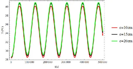
[image:5.595.304.549.312.405.2]It is should be noticed that this new analytical solution converge very quickly. Few numbers of terms are sufficient to have a good accuracy. In this work we use the first four terms (n=4). The analysis of the results of figure 3, can validate this choice.
Fig. 3.The effect of number of terms n on the result accurate: (h1=40 h2=30 e=40 cm x=0 cm a=9×10⁻⁷m2/s
λ=1.7)
B. Comparison with solution derived from the Laplace transform technic
The validation of the analytical solution has been carried out with a semi analytical solution obtained by numerical inversion of the Laplace transform.
First the initial condition is reformulated as:
1 2
2 1 2 1
i s a
1
1 2 1 2
2 1 2
i s a
2
1 2 1 2
T x, 0 A x A with
h h h h
.T .T 0
A
h h h h
.e
h h h
1 .e .T .T 0
A
h h h h
.e
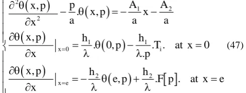
And then we apply the Laplace transform according to the variable time t on Eq.(8) (9) and (10) we obtain the following system
2 1 2 2 1 1x 0 i
2 2
x e
A
A
p
x, p
.
x, p
x
a
a
a
x
x, p
h
h
.
0, p
.T . at x
0
x
.p
x, p
h
h
e, p
.F p . at x
e
x
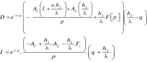
(47)The solution of Eq.(47) in Laplace space can be written as :
q .x q .x
e .q 1 2 e .q 2 1
2 1 2 1
i s a
1 2 1 2
2 1 2
i s
W L .e D I .e
x , p
h h h h
e q q e q q
h h h h
.T .T 0
1
. x
p h h h h
.e
h h h
1 .e .T .T
1 . p
a1 2 1 2
0
h h h h
.e
(48) With: 1 1
1 2 i
e .q 2
h h
A .A .T
h
W .e q
p 2 2 1 2 2 1 e.h h
A 1 A
h h
L F p . q
2 2
1 2
e .q 2 2
e.h h
A 1 A
h h
D e F p q
p
1 1
1 2 i
e .q 2
h h
A .A .T
h
I e . . q
p
With F[p] is the Laplace transform of the sol air temperature Ts-a(t) (Eq.(11)).
The solution T(x,t) in the reel space is obtained by inversing numerically (Eq.(48)) using the Zakian method [15,16,17].This method was chosen because it converges very quickly and it is easy to implement on the computer. It doesn’t need any additional arbitrary regularization constant. In the case of functions with oscillatory behaviors (our case), the Zakian method is applicable with acceptable accurate at low time range[18].That is sufficient to study the validation of the analytical solution.
Zakian's algorithm approximates the solution in the reel space using the following equation:
nj j th
j
ma i
1
1 i 2
T ( x ,t ) e,T ,a,b ,
t b , 2
Re K t
(49)
For n=5 the constants Kj and αj are listed in [15] Where :
i
1
[image:6.595.48.285.51.153.2]The figures 4 and 5 show the curves given by the new analytical solution and the solution obtained by numerical inversion using Zakian method. As we can see there is a good agreement between the two solutions. This validate the obtained analytical solution which in addition, it less time consuming.
Fig. 4.Comparison between the analytical and the numerical solutions (h1=7.7 h2=25 e=30 cm x=30cm
a=3.6×10⁻⁷m2/s λ=0.46)
Fig. 5.Comparison between the analytical and the numerical solutions (h1=4 h2=3 e=20 cm x=20cm
[image:6.595.311.552.51.164.2]a=3.6×10⁻⁷m2/s λ=0.46) IV. RESULTS ANDDISCUSSION
Table- I: The thermophysical properties of the used materials
Sample λ [W.m-1.K-1]
a×10-7 [m2.s-1]
Cp
[J/(kg.K)] ρ [kg/m3] Clay (CT) 0.368 3.22 706.8 1616.83 Clay (CE) 0.34 2.99 705.9 1616.16 Clay(CM) 0.457 3.503 690 1890.25 Expanded
cork [20] 0.038 2.44 1560
100
A. Dynamic thermal characteristics as a function of the wall thickness
Thermal resistance is a heat property and a measurement of a temperature difference by which an object or material resists a heat flow.
Figure 6 shows that the thermal resistance increases linearly with increasing wall thickness.
[image:6.595.53.294.504.612.2]Earthen wall adduce thermal storage capacity but little insulation performance (low R-value).Figure 6 indicates that for a large thickness wall, the thermal resistance is lower than the value required by the Moroccan Thermal Regulation of Construction (MTRC). The use of a wall, purely constructed of unfired clay bricks, need the use of a complementary insulation to reach the target values of thermal resistance requested in the MTRC.
Fig. 6.Variation of thermal resistance as a function of wall thickness for the three types of unfired clay brick.
This paragraph is devised into two part, The first part aims to evaluate the dynamic thermal characteristics of wall purely constructed from three types of unfired clay bricks in order to determine the optimum thickness wall to achieve a highest values of thermal inertia. The presence of mortar joints used for built unfired clay brick wall
[image:6.595.308.554.530.649.2]International Journal of Innovative Technology and Exploring Engineering (IJITEE) ISSN: 2278-3075,Volume-8 Issue-12, October 2019
The effects of outer and inner combined convection and radiation heat transfer coefficient and thickness wall on the dynamic thermal behaviors, are studied in this part. After identification of the optimum thickness of earthen wall we will discuss in the second part the effect of application thermal insulation on the energy performance. The thickness of thermal insulation is determined in order to reach the target values of thermal resistance of external wall in (MTRC).
According to the results presented in figure 7 it is noticed that the decrement factor decreases with increasing thickness wall. This result is explained by the fact that increasing the thickness increases the resistance to heat transfer from the outside to the inside. so the amount of heat transfer across the wall decreases with thickness. Figure 8 shows that the thickness makes it possible to damp the fluctuations of the thermal wave coming from outside. Peak-to-peak amplitude of the internal temperature decreases with the thickness. However, Peak-to-peak amplitude of the external temperature is almost constant (figure 9). consequently, the decrement factor decreases with increasing thickness.
[image:7.595.316.543.107.226.2]from figure 8, it should be noticed that for a thickness higher than 0.4m a large part of fluctuation is damped and the internal temperature becomes stable and almost constant (low value of decrement factor). So exceeding this value is unnecessary.
Fig. 7.The effect of wall thickness on the decrement factor for the three types of unfired clay bricks
Fig. 8.The effect of wall thickness on the internal temperature for the unfired clay brick (CM) However reducing the decrement factor can improves energy efficiency and reduces the energy consumption of earthen construction. The obtained results in this work demonstrate that reducing decrement factor has the effect of decreasing daily peak fluctuations of the thermal wave coming from outside which may decrease energy consumption in two ways. First, the attenuation of external temperature fluctuation will minimize the overall energy needed to maintain an interior set point temperature. Second,
this effect can reduce the size requirements of the building heating and air conditioning equipment. Consequently, enabling these equipments to run at more efficient operating loads.
[image:7.595.53.291.385.643.2]Fig. 9.The effect of wall thickness on the external temperature for the unfired clay brick (CM) Time lag as function of thickness wall of the three types of unfired clay bricks is shown in figure 10. It increases quasi-linearly with increasing wall thickness. Increasing wall thickness retards the penetration of the exterior thermal load wave inside the interior ambiance. The raison of this result is that the thermal storage and absorption capacity of wall increases with thickness. The analysis of the results in figure 8 demonstrate that the maxima position of the internal temperature is shifted from the left to the right with the increases in thickness (phase lag increases). While this position remains almost fixed for the external temperature (figure 9).Consequently, the time lag increases with increasing thickness.
Fig. 10. The effect of wall thickness on the time lag for the three types of unfired clay bricks
The heat flux during 24 hours at the inner surface (x=0) is calculated by :
t 24 h
x 0 0
T x ,t
Q
.dt
x
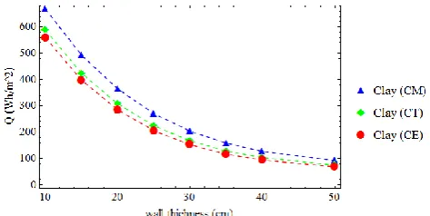
(50) [image:7.595.305.550.432.562.2]Fig. 11. Wall thickness effect on heat flux during a day (24 hours) for the three types of unfired clay bricks In order to limit the risk of overheating during hottest period, It is noticed that the time lag must be have a values between 10 and 12 hours [5]. In this work the optimum thickness is defined as the thickness that conduct a low value of decrement factor and a time lag between 10 and 12 hours. The results show that the ideal thickness to reach the desired parameters of thermal inertia is between 30 cm and 35 cm for the unfired clay bricks (CT) and (CE) and between 30 cm and 40 cm for the unfired clay brick (CM).
A similar conclusion on the effect of thickness on time lag and decrement factor has reported by several researchers[5][8].
B. Dynamic thermal characteristics as a function of the outer and inner combined convection and radiation heat transfer coefficient
Figures 12 and 14 show the variation of the decrement factor and the time lag as a function of inside combined convection and radiation heat transfer coefficients h1. In order to illustrate the influence of h1 the values of h2 is fixed at (h2=25W/m2.K and different values of h1 are considered for various wall thickness mad from the unfired clay brick (CM).The results shows that h1 affect significantly the dynamic thermal characteristics.
As shown in Fig 12 that as the decrement factor decreases with the increase in the inside combined convection and radiation heat transfer coefficient h1. This result can be explained by the fact that the increase in h1 increases the convective heat flow at the inner surface, which leads to an increase in the cooling rate whereas, the fluctuation of inside temperature damps significantly. The figure 13 demonstrate this effect. Consequently, the decrement factor decreases with the increase in h1.
[image:8.595.315.543.53.181.2]Fig. 12. Inside combined convection and radiation heat transfer coefficient effect on the decrement factor for different wall thickness of the unfired clay brick (CM)
Fig. 13. Inside combined convection and radiation heat transfer coefficient effect on the internal temperature
(unfired clay brick (CM)).
As seen as from fig 14 that the time lag decreases with h1. For wall thickness smaller than 40 cm the relationship between decrement factor and time lag with h1 can be divided into the three separate parts. The first part corresponds to h1 < 25W/m2.K. In this case time lag and decrement factor depends severely on the variation of h1. In the second part time lag and decrement factor depends slightly on h1 (correspond to 25<h1<40 )whereas in the third part time lag and decrement factor goes to be almost constant and can be considered independent of h1 (correspond to h1>40 W/m2.K).
[image:8.595.310.549.563.683.2]For wall thickness higher than 40 cm time lag and decrement factor can be considered independent of h1.
Fig. 14. Inside combined convection and radiation heat transfer coefficient effect on the time lag for different wall
[image:8.595.56.282.612.734.2]thickness of the unfired clay brick (CM).
Fig. 15. Outside combined convection and radiation heat transfer coefficient effect on the decrement factor for
International Journal of Innovative Technology and Exploring Engineering (IJITEE) ISSN: 2278-3075,Volume-8 Issue-12, October 2019
The effect of outdoor heat-transfer coefficient h2 on time lag and decrement factor is presented in figures 15 and 16. to highlight this effect the values of h1 is fixed (h1=7.7 W/m2.K) while various values of h2 and different thickness are investigated for wall built from the unfired clay brick (CM). The results show that the time lag and the decrement factor is almost constant and independent on the variation of h2.
[image:9.595.313.541.96.208.2]
Fig. 16. Outside combined convection and radiation heat transfer coefficient effect on the time lag for different wall thickness of the unfired clay brick (CM). C. Dynamic thermal characteristics as a function of the thermal insulation thickness
The methodology presented in Salazar [19] for calculating the equivalent thermophysical properties of a multilayer wall is adopted here, to examine the effect of thermal insulation on the dynamic thermal characteristics of earthen walls.
According to [19] the equivalent thermal conductivity is define as:
effe
1 2
1 2
1
(51)
Where v1and v2 represent the volumetric proportion of the wall made from unfired clay brick and the insulating layer respectively
1
1
1
1 1 2 2
e
S
e
S
e
S
(52)
2 2 2
1 1 2 2
e
S
e
S
e
S
(53)
And
effe 1 2
1 2
1 2
1
e e
e e
(54)
The equivalent heat capacity per unit volume and the equivalent thermal diffusivity are then:
1 p 1 2 p 2 p effe 1 p 1 2 p 2
1 2
e
.C
e
.C
.C
.C
.C
e
e
(55)
effe effe
p effe
a
.C
(56)
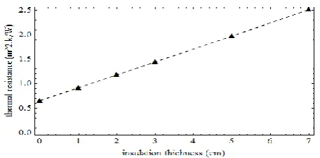
Figure 17 shows that the thermal resistance increases linearly with increasing insulation thickness. So adding an insulating layer to the earthen wall decreases the amount of heat transfer across the wall. It is noticed that a wall with 5 cm
of thermal insulation meets the MTRC requirements which stipulates for Marrakech a thermal transmittance inferior than 0.55 w.m-2.k-1
Fig. 17. Variation of thermal resistance as a function of thermal insulation thickness for the unfired clay brick
(CM).
It is clear from Fig 18 that as the decrement factor decreases with the increase in the insulation thickness. The decrement factor is reduced about 91% for wall with 5 cm of insulation layer. Adding an insulation layer to the earthen wall acts as a barrier of exterior thermal load wave and permits to damp a large part of the temperature fluctuation. Consequently, the internal temperature becomes stable and almost constant(figure 19).
Fig. 18. the effect of thermal insulation thickness on the decrement factor
Fig. 19. the internal temperature (5cm of insulation)
[image:9.595.51.289.144.274.2] [image:9.595.281.555.328.739.2]As seen from Figure 20, Using an insulation layer causes a decrease in heat flux Q during 24 hours at the inner surface. Consequently, the energy consumption of earthen construction would be reduced by Adding an insulation layer.
V. CONCLUSION
This work presents theoretical and experimental investigations to evaluate the thermophysical properties and the energy performance of earthen walls mad from three types of unfired clay bricks. From the results, it can be noted the conclusions below :
1. Wall thickness and the inner combined convection and radiation heat coefficient (h1) affect significantly the decrement factor and the time lag.
2. Time lag and decrement factor almost constant and independent on the variation of the outer combined convection and radiation heat coefficient (h2).
3. For wall thickness higher than 40 cm time lag and decrement factor can be considered independent of h1.
4. For wall thickness smaller than 40 cm time lag and decrement factor decreases with increase in h1. For h1 < 25 W/m2.K time lag and decrement factor depends severely on the variation of h1.While time lag and decrement factor depends slightly on the variation of h1 for 25 ≤ h1 ≤ 40 W/m2.K. Therefore, for h1>40 W/m2.K time lag and decrement factor can be considered independent of h1.
5. The optimum thickness to achieve a highest value of thermal inertia (low value of decrement factor and time lag between 10 and 12 hours) for the walls mad from the three types of unfired clay bricks was identified between 0.3m and 0.4m.
6. Decrement factor decreases with increase in thermal insulation thickness.
ACKNOWLEDGMENT
The present research study is part of the λ@DB project which aims to develop a national database of the thermophysical properties of the main local building materials in Morocco, supported by the German International Cooperation (GIZ). REFERENCES
1. Chel, A., Tiwari, G.N. Thermal performance and embodied energy analysis of a passive house: Case study of vault roof mud-house in India. Applied Energ, 86 (2009) 1956-1969.
2. Shukla, A., Tiwari, G.N., Sodha, M.S. Embodied energy analysis of adobe house. Renewable Energy 34 (2009): 755–761.
3. Martin, S., Mazarron, F. R., Canas, I. Study of thermal environment inside rural houses of Navapalos (Spain): The advantages of reuse buildings of high thermal inertia. Construction and Building Materials 24 (2010): 666-676.
4. Zami, M.S., Lee, A. Economic benefits of contemporary earth construction in low-cost urban housing – State-of-the-art review. Journal of Building Appraisal, 5 (2010): 259-271.
5. El Fgaier, F., Lafhaj, Z., Antczak, E., & Chapiseau, C. (2016). Dynamic thermal performance of three types of unfired earth bricks. Applied Thermal Engineering, 93, 377-383.
6. El Fgaiera F, Lafhaj Z, Brachelet F, Antczak E, Chapiseau C. Thermal performance of unfired clay bricks used in construction in the north of France. Case Studies in Const Mater 2015; 3: 102–111
7. M. Ozel, Thermal, economical and environmental analysis of insulated building walls in a cold climate, Energy Conversion and Management, Vol. 76, pp. 674–684, 2013.
8. Asan, H. (2006). Numerical computation of time lags and decrement factors for different building materials. building and environment, 41(5), 615-620.
9. Ozel, Meral. "Determination of optimum insulation thickness based on cooling transmission load for building walls in a hot climate." Energy Conversion and Management 66 (2013): 106-114.
10. Al-Sanea, Sami A., M. F. Zedan, and S. N. Al-Hussain. "Effect of thermal mass on performance of insulated building walls and the concept of energy savings potential." Applied Energy 89.1 (2012): 430-442.
11. Ulgen K. Experimental and theoretical investigation of effects of wall’s thermophysical properties on time lag and decrement factor. Energy Build2002;34:273–8.
12. Asan H. Investigation of wall’s optimum insulation position from maximum time lag and minimum decrement factor point of view. Energy Build2000;32:197–203.
13. Kaşka, Önder, Recep Yumrutaş, and Orhan Arpa. "Theoretical and experimental investigation of total equivalent temperature difference (TETD) values for building walls and flat roofs in Turkey." Applied Energy 86.5 (2009): 737-747.
14. Available: http://www.marocmeteo.ma
15. ZAKIAN, V. (1969). Numerical Inversion of Laplace Transform, Electronic Letters, Vol. 5, No. 6, pp. 120-12
16. ZAKIAN, V. (1970a). Rational Approximation to TransformFunction Matrix of Distributed System, ElectronicLetters, Vol. 6, No. 15, pp. 474-476
17. Yassine Chihab, Mohammed Garoum, Najma Laaroussi, Thermophysical characterization of earthen materials using the flash method, 2019. DOI: 10.35940/ijitee.K1801.0981119
18. Hassanzadeh, Hassan, and Mehran Pooladi-Darvish. "Comparison of different numerical Laplace inversion methods for engineering applications." Applied mathematics and computation 189.2 (2007): 1966-1981.
19. Salazar, A., On Thermal Diffusivity. European Journal of Physics, 2003. 24(4): p. 351.
20. Tadeu, A., et al. "Thermal delay provided by floors containing layers that incorporate expanded cork granule waste." Energy and buildings 68 (2014): 611-619.
21. Chihab, Yassine, et al. "The Effect of Clay Consistency on the Thermophysical Properties of Composite Material Clay-straw." 2018 6th International Renewable and Sustainable Energy Conference (IRSEC). IEEE, 2019.