On the approximation of spatial structures of global tidal magnetic field models

https://doi.org/10.5194/angeo-36-1393-2018 © Author(s) 2018. This work is distributed under the Creative Commons Attribution 4.0 License.

On the approximation of spatial structures of global

tidal magnetic field models

Roger Telschow1, Christian Gerhards1, and Martin Rother2

1_{Computational Science Center, University of Vienna, 1090 Vienna, Austria}

2_{Helmholtz Centre Potsdam German Research Centre for Geosciences – GFZ, Section 2.3 Geomagnetism,} 14467 Potsdam, Germany

Correspondence:Roger Telschow ([email protected]) Received: 29 June 2018 – Discussion started: 10 July 2018 Accepted: 1 October 2018 – Published: 18 October 2018

Abstract.The extraction of the magnetic signal induced by the oceanic M2 tide is typically based solely on the tempo-ral periodicity of the signal. Here, we propose a system of tailored trial functions that additionally takes the spatial con-straint into account that the sources of the signal are localized within the oceans. This construction requires knowledge of the underlying conductivity model but not of the inducing tidal current velocity. Approximations of existing tidal mag-netic field models with these trial functions and comparisons with approximations based on other localized and nonlocal-ized trial functions are illustrated.

1 Introduction

Conductive seawater moving through the ambient Earth’s main magnetic field Bmain induces a secondary magnetic fieldBoc. Due to their periodic nature, magnetic signals gen-erated by ocean tides are particularly easy to detect and have been studied in observatory data as early as, e.g., Malin (1970). However, the extraction of global models for mag-netic fields induced by the dominating M2 tide from satellite data has only recently become possible (e.g., Sabaka et al., 2015, 2016; Tyler et al., 2003). Although the extraction pro-cedures used are solely based on the temporal periodicity of the tidal signal (and not on further information on the spatial localization of the sources), they seem, by visual inspection, to coincide very well with results obtained by forward mod-els such as in Kuvshinov and Olsen (2005). A more exten-sive comparison of forward models of electromagnetic ocean tidal signals based on different ocean tide models has

re-cently been published in Saynisch et al. (2018). In that work, it was shown that the residuals between the different mod-els can exceed the nominal noise level of the Swarm satel-lite mission. The ability to extract M2 tidal magnetic field signals in satellite data more precisely can therefore help in constraining ocean tide models. In Grayver et al. (2016) and Schnepf et al. (2015) it has been shown that an M2 tidal magnetic field model can also be used to constrain 1-D mod-els of the Earth’s mantle conductivity, and forward studies in Irrgang et al. (2016) have shown that lateral variations in the conductivity of the ocean water itself should have a de-tectable influence on the measured magnetic field (although the latter study was performed for general ocean circulation and not for tidal current systems).

In this short paper, we want to illustrate the effects that different (spatially localized) sets of trial functions can have on the approximation of the magnetic field induced by the M2 tide in the first place.

lying conductivityσ, and the frequencyω. Furthermore,E

denotes the electric field andµ0is the vacuum permeability. Instead of using a fixed velocity fieldu, we substitute it by a set of functions{u_{`</sub>}<sub>`=1,...,L}(e.g., vectorial Slepian functions as in Plattner and Simons (2014, 2015) that are localized over the oceans) to obtain a set of corresponding trial functions

{B`}`=1,...,Lthat each solve Eq. (1). The latter is suitable for the approximation ofBocand reflects the spatial localization of the sources of the induced magnetic signal in the oceans. Thus, a magnetic field model that is based on an expansion of the signal in terms of the function system{B`}`=1,...,L au-tomatically reflects the spatial origin of the signal as well as its temporal periodicity (described by the frequencyω). Ad-ditionally, due to the linear connection between uandBoc, an approximation ofBocdirectly yields an approximation of the underlying tidal current velocityuin terms of the func-tions{u`}`=1,...,L. However, a model of the underlying con-ductivityσhas to be assumed for the construction of theB`. Throughout this paper, we fix the underlying conductivity, meaning that we do not test the influence of a variation of the conductivity model on the approximation ofBoc. The goal of the paper is rather the illustration of the effect of the general constraint that the (unknown) underlyinguis restricted to the oceans. In a forthcoming study, the simultaneous reconstruc-tion ofuand approximation ofBoc, and a comparison with existing models, shall be investigated more thoroughly. Since the connection betweenσ andBocis nonlinear, a simultane-ous determination of σ andBoc(assuming a fixed velocity field model foru) is not as straightforward. A detailed de-scription of the trial functions is provided in Sect. 2.

In Sect. 3, we illustrate our approach with input data de-rived from the (satellite- and observatory-data-based) CM5 model of Sabaka et al. (2015) and from data derived from a forward model based on the X3DG solver from Kuvshinov (2008). We approximate these input data sets separately in terms of time-periodic vector spherical harmonics, a system of spatially localized trial functions that contains no particu-lar information on the underlying sources (in our case, Abel– Poisson kernels), and the new set of trial functions indicated in the previous paragraph, respectively. We also include an example with artificial continental noise. The residuals with respect to the input data show that the use of the function sys-tem{B`}`=1,...,Lcan filter out undesired contributions to the M2 tidal magnetic field over the continents, without neglect-ing data over the continents. These residuals can reach up to 15% of the maximal signal strength and have a magnitude that should be detectable at satellite altitude.

BN= i=1

αidi

ofBocby iteratively choosing coefficientsαi∈Rand dictio-nary elementsdi∈Dvia

argmin_α,dkRi−1−αFdk2

RM+λkBi−1+αdk 2 H

. (2)

Ri−1=b−FBi−1 denotes the residual between the data

b∈_RM and the approximation afteri−1 iterations. In this particular setup,F represents the linear operator that evalu-ates a function at theM locations where data are provided, andHis a suitable Hilbert space for the regularization of the problem1. The parameterλcontrols the trade-off between the data misfitkRik2

RM and the regularizing termkBik 2 H, which imposes a certain property toBi such as smoothness (as in our case). The Regularized (Orthogonal) Functional Match-ing Pursuit, in general, has the advantage that it can easily deal with different dictionariesD(or combinations of such) from which the approximantBNis built. However, any other approximation method could be used as well with the pro-posed function systems. In this paper, we use the term “dic-tionary” simply to describe a set of arbitrary functions that we consider suitable for our purposes. These functions do not necessarily have to satisfy particular mathematical prop-erties such as orthogonality or completeness. Therefore, we call such functions “trial functions” rather than, e.g., “basis functions”.

In the following, we briefly introduce some function sys-tems that can be used for the constitution ofD. In particular, Sect. 2.4 describes in more detail the aforementioned trial functions{B`}`=1,...,Lthat contain temporal and spatial con-straints tailored for ocean-tide-induced magnetic fields. 2.1 Vector spherical harmonics

We briefly recapitulate the notion of classical vector spheri-cal harmonics in a form that we need at a few occasions later on. BySr= {x∈R3: |x| =r}, we denote the sphere of ra-diusr, while S=S1 stands for the unit sphere. Every unit vectorξ =ξ(t, ϕ)∈_Scan be expressed in spherical coordi-nates with longitudeϕ and polar distancet=cos(ϑ ), where ϑis the corresponding co-latitude. ByYn,k, we denote fully

1_{In our case, we use the normkfk}2 H=

P

n,k(n+12)4fˆ(n,k), but other norms can be used as well depending on the property one wants to impose onf. By_fˆ

Figure 1.The kernelK(r·, aη1)forar =0.91(a)andar =0.67(b). The fixed nodal pointη1∈Sis marked by a white cross.

Figure 2.Absolute value of the vectorial Slepian functiong(₅₀3)with 50th best localization over the oceans(a)andg(₁₆₃₀3) with the 50th worst localization over the oceans(b), for bandlimitN=40.

normalized spherical harmonics of degreenand orderk: for everyn∈_N0andk= −n, . . ., n,

Yn,k(ξ )=

s 2n+1

4π

(n− |k|)!

(n+ |k|)!P |k|

n (t )

 

 √

2 cos(kϕ), k <0,

1, k=0,

√

2 sin(kϕ), k >0. The involved associated Legendre functions are, for t∈ [−1,1], defined as

P_nk(t )=(−1) k

2n_n!

1−t2k/2 _d

dt n+k

(t2−1)n.

Iff is a scalar-valued square-integrable function onS, then, for every degreen∈_N0and orderk= −n, . . ., n, the values

ˆ

f(n,k)= Z

S

f (η)Yn,k(η)dS(η) (3)

are called the Fourier coefficients of the functionf.

Going over to the vectorial setting, it is well known that every square-integrable vector fieldf on the unit sphere can be uniquely decomposed into its radial and two tangential components such that

f =erf1+ ∇Sf2+LSf3,

with scalar-valued functions f1, f2, f3 and the radial unit vector er=

√

1−t2_cos(ϕ),√_1−t2_{sin(ϕ), t}T_{. By the} surface gradient∇

S, we denote the tangential component of the usual Euclidean gradient∇, i.e.,

∇ S=eϕ

1

√

1−t2 ∂ ∂ϕ+et

p 1−t2∂

∂t,

with unit vectorset=

−tcos(ϕ),−tsin(ϕ),

√

1−t2T _and

e_ϕ=(−sin(ϕ),cos(ϕ),0)T. Moreover, the surface curl gra-dientL_Sis defined byL_Sf (ξ )=ξ×∇

Sf (ξ ), where×is the usual cross product inR3. In other words,

L_S= −eϕ p

1−t2∂ ∂t +et

1

√

1−t2 ∂ ∂ϕ.

Hence, we define three types of vector spherical harmonics: the radial

y(_n,k1) =erYn,k,

for degrees n≥0 and ordersk= −n, . . ., n, as well as the tangential

y(_n,k2) = s

1

n(n+1)∇SYn,k, (4)

y(_n,k3) = s

1

n(n+1)LSYn,k, (5) for degrees n≥1 and orders k= −n, . . ., n. Note that, for convenience, we set y(₀2_,)₀=y(₀3_,0)=0. It should further be noted that the vector spherical harmonics in Eq. (4) are curl-free while those in Eq. (5) are surface-divergence-free. In analogy to Eq. (3), we can now define the Fourier coefficients

ˆ

f_(n,k)(i) = Z

S

monics:

h_n,k(x)= 1

r2 a

r n

∇

SYn,k(ξ )−ξ(n+1)Yn,k(ξ )

, (6) for r= |x|> a andξ = x

|x| ∈S, wherea is the radius of a reference sphere, e.g., Earth’s mean radius.

2.2 Vectorial Abel–Poisson kernel

While the set of functions{h_n,k}_{n∈N0,k=−n,...,n} from Eq. (6) is suitable for the global approximation of potential field data, we are also interested in localized functions. One pos-sible choice is the Abel–Poisson kernel (see, e.g., Freeden and Gerhards, 2012; Freeden et al., 1998). For x, y∈_R3,

|x|>|y|, it is defined by K(x, y)= 1

4π

|x|2− |y|2 |x−y|3 .

That is, with unit vectors ξ, η∈_S and radii r > a >0, we have

K(rξ, aη)= 1

4π

r2−a2

a2_+r2_{−2ar(ξ·η)}3/2,

which shows thatK only depends on the spherical distance betweenξandη, since|ξ−η|2=2(1−ξ·η). Therefore, the kernel is radially symmetric if we keep one of the variables fixed (we strictly keep the second argument fixed, hereaη). The degree of localization is determined by the ratio a_r. The closer it is to 1, i.e., the smaller the difference between the radiia andr, the better the spatial localization ofK(r·, aη) around η. In our case, we choosea to be the Earth’s mean radius, andris the radius of the sphere at which we evaluate the kernel. An illustration of the kernel is provided in Fig. 1. The corresponding vectorial Abel–Poisson kernel is sim-ply defined by

k(x, y)= ∇_xK(x, y)= 1

4π ∞ X n=0 n X

k=−n Yn,k

y

|y|

hn,k(x).

Further calculations show

k(x, y)= 1

4π

₂

|x−y|3x − 3

|x|2− |y|2 |x−y|5 (x−y)

. (7) A spatially localized alternative to{hn,k}n∈_N0,k=−n,...,ncould then be defined by the set of functions {k(·, aηi)}i=1,...,M, whereη1, . . ., ηM∈Sis a fixed set of adequately distributed nodal points.

for details).

Specifically, the functionf showing the best localization in0, is the one that maximizes the energy ratio

λ0(f)= R

0|f(η)|2dS(η) R

S|f(η)|

2_dS(η), (8)

i.e., the one with an energy ratio closest to 1. Let us now assume thatg(i)_{is a bandlimited vectorial function of typei} with bandlimitN; i.e., it can be expanded as

g(i)= N X

n=0 n X

k=−n ˆ

g(i)_(n,k)y(i)_n,k.

Further, the matrixP=(P(n,k),(m,j ))∈R(N+1)2×(N+1)2 con-tains (properly sorted2) all of the appearing inner products P(n,k),(m,j )=

Z

0

y(i)_n,k(η)·y(i)_m,j(η)dS(η)

and gˆ =(gˆ_(n,k)(i) )T∈_R(N+1)2, with n=0, . . ., N and k= −n, . . ., n. If we now restrict ourselves to normalized func-tions g(i) (i.e., R

S|g

(i)_(η)|2_{dS(η)= ˆg}T_{gˆ=1), one obtains} the simple expression λ0(g(i))= ˆgTPgˆ. Eventually, the maximization of the energy ratio Eq. (8) leads to the eigen-value problem

Pgˆ=λgˆ.

The eigenvalues λ` are the possible energy ratios and the corresponding eigenvectors gˆ<sub>`</sub> contain the Fourier coeffi-cients of bandlimited functionsg(i)<sub>`</sub> attaining the energy ratio λ`=λ0

g(i)_{`</sub> . The set of functions{g(i)<sub>`} }

`=1,...,(N+1)2 is or-dered such that 1≥λ1≥λ2≥. . .≥λ_(N+1)2≥0.

In typical scenarios, it turns out that the eigenvalues are clustered close to 1 and close to zero. Those eigenval-ues λ1, . . ., λL which are closer to 1 determine the subset {g(i)_{`</sub> }<sub>`=1,...,L}of well-localized Slepian functions that should be used for approximation in0. The code for the genera-tion of vectorial Slepian funcgenera-tions has been kindly supplied in Plattner and Simons (2017b). For our situation, where0 denotes the region of (a spherical) Earth which is covered by oceans, an illustration is provided in Fig. 2.

Figure 3.Absolute value of the trial functionBre₅₀corresponding tou=g₅₀(3)at timet=0(a)and the trial functionBre₁₆₃₀corresponding to

u=g(₁₆₃₀3) at timet=0(b). Models of surface shell conductance onSaand absolute value ofBmainonSaused for the generation of the trial functions(c, d).

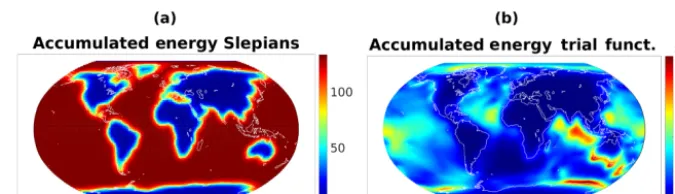
Figure 4.Accumulated energy for{u`}`=1,...,L(a)and{B_{`</sub>re,Bim<sub>`} }`=1,...,L(b), withL=1200.

2.4 Physics-based trial functions

We start with the time-harmonic Maxwell equations as al-ready indicated in Eq. (1). For simplicity, we assume a 1-D (only radially varying) conductivity model forσ within the ball Ba, and at the surfaceSa we allow a laterally varying conductivity (cf. the bottom left image in Fig. 3 for an illus-tration). Further, the magnetic fieldBmainis taken from the CHAOS-5 model (see Finlay et al., 2015) anduis supposed to denote a depth-integrated velocity field that is restricted toSa(in fact, within the numerical framework of the X3DG solver, we assume a constant ocean depth of 1km, withu be-ing tangential to the sphere and independent of the depth). Since we are mainly interested in tidal velocity fields, it is a reasonable assumption that uis surface-divergence-free for most parts of the oceans. The latter means thatucan be ex-panded in terms of vector spherical harmonics or vectorial Slepian functions of type 3, i.e.,y(_n,k3) org(_`3), respectively.

For the generation of the tailored trial functions

{B`}`=1,...,L, we therefore substituteuby a set of surface-divergence-free functions{u`}`=1,...,Lthat reflect spatial

lo-calization within the oceans. More precisely, we choose

u`=g(`3),

whereg(<sub>`</sub>3)is the`th best localized vectorial Slepian function of type 3. The corresponding solutionBocof Eq. (1) within this setup then provides an auxiliary functionBe`. It should be noted that in order to obtain Maxwell’s equation in the time-harmonic form Eq. (1), one has to apply a Fourier transform in time. Therefore, for the actual trial functionB`, we have to invert the Fourier transform and get

B`(x, t )=e−iωtBe`(x), x∈R3, t∈R.

For technical reasons, we choose to work in a real-valued framework, so that the real and imaginary part ofB` each yield a trial function

Bre_`(x, t )=cos(ωt )eB re

`(x)+sin(ωt )Be im

` (x), (9)

Bim_` (x, t )=sin(ωt )Be re

`(x)−cos(ωt )eB im

` (x). (10)

Figure 5.Absolute value of the radial part of the tidal modelBCM5_oc as well as the forward modelBX3DG_oc at an altitude of 300 km above the Earth’s surface.

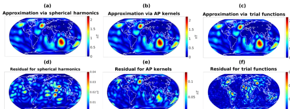
Figure 6. Absolute value of the radial part of approximations ofBCM5_oc based on dictionaryD1(a), dictionaryD2(b), and dictionary

D3(c), as well as the corresponding residuals with respect toBCM5oc (d, e, f). Note the different scales in the bottom row which are chosen in order to emphasize the spatial distribution of the residuals.

as well as the spatial localization of the sources within the oceans. An illustration for the M2 tide withω= 2π

12.42h can be found in Fig. 3. For the computation of theBe`as solutions of Eq. (1), we have used the X3DG solver from Kuvshinov (2008).

Figure 4 shows the accumulated energyPL_{`=1</sub>|u`(ξ )|2, for ξ ∈_S, of the underlying functionsu` that describe the ve-locity field and the accumulated energyPL<sub>`=1}|Bre_{`</sub>(x, t )|2+ |Bim<sub>`} (x, t )|2, forx∈_Sr withr=a+300 km and timet=0, of the corresponding trial functions. In both cases, one can clearly see the spatial localization over the oceans. However, the accumulated energy of the trial functions additionally re-flects the influence of the conductivityσ and the main/core magnetic fieldBmainindicated in Fig. 3.

3 Examples

For our experiments we rely on the CM5 geomagnetic field model (cf. Sabaka et al., 2015) and a forward model based on the M2 depth-integrated tidal velocity field from

TPXO8-ATLAS (cf. Egbert and Erofeeva, 2002) that has also been used in Kuvshinov (2008). The contribution of CM5 that is due to the oceanic M2 tide is given as an expansion in terms of spherical harmonics up to degree 18; we denote it asBCM5_oc for the remainder of this section and sample it atM=250 000 points which are taken from actual Swarm satellite tracks. The forward model has been computed via the X3DG solver based on the surface conductance and the main/core magnetic field model indicated in the bottom row of Fig. 3 and a depth-integrated M2 tidal velocity field from TPXO8-ATLAS. We denote it byBX3DG_oc and evaluate it on the same point grid as before. These samples are used as input datab∈_RM for the Regularized (Orthogonal) Func-tional Matching Pursuit, which works iteratively as indicated in Eq. (2). In the following, we want to illustrate the influence of the choice of different function systems (i.e., the choice of different dictionariesD)on the approximation ofBCM5_oc and

BX3DG_oc . For that purpose, we choose three different dictio-naries: the spherical-harmonic-based

Figure 7.Absolute value of the radial part of approximations ofBX3DG_oc based on dictionaryD1(a), dictionaryD2(b), and dictionaryD3

(c), as well as the corresponding residuals with respect toBX3DG_oc (d, e, f).

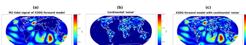
Figure 8.Absolute value of the radial part ofBX3DG_oc (a)and model of continental “noise”e(b), as well as superpositionBe_ocof both of these(c).

with ω= 2π

12.42h and the functions hn,k from Eq. (6); the Abel–Poisson-kernel-based

D2= {cos(ωt )k(x, aηi),sin(ωt )k(x, aηi)}i=1,...,Mp, where a=6371.2 km, {ηi}i=1,...,Mp is a Reuter grid on S withMp=6201 nearly equally distributed points (see, e.g., Michel (2013), p. 137), andkgiven as in Eq. (7); and

D3= {Bre`(x, t ),B im

` (x, t )}`=1,...,1200,

with Bre

` and Bim` , the physics-based trial functions from Eqs. (9) and (10).

The actual signals that we want to approximate are indi-cated in Fig. 5. The approximationsBN of BCM5oc together with the residuals |BN−BCM5oc | for each of the three dic-tionaries above are shown in Fig. 6, whereas the respec-tive approximations ofBX3DG_oc and corresponding residuals

|BN−BX3DGoc |are displayed in Fig. 7.

In the case ofBCM5_oc as the underlying signal, it can be seen in Fig. 6 that the dictionaryD1yields the overall best approx-imation, which, however, is not surprising since we try to fit a based model with a spherical-harmonic-based dictionary. The result for dictionaryD2shows a more

resid-Figure 9.Absolute value of the radial part of approximations of superpositionBe_oc based on dictionaryD1(a), dictionaryD2(b), and dictionaryD3(c), as well as the corresponding residuals with respect to originalBX3DGoc without the continental “noise”e(d, e, f).

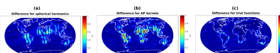
Figure 10.The difference between the approximationsBNof the undisturbedBX3DGoc (as shown in Fig. 7a, b, and c) and the approximations

Be_Nof the noisyBe_oc(as shown in Fig. 9a, b, and c).

uals over the continents show that the use of the adapted trial functions might eventually deliver improved tidal magnetic field models that correct unrealistic continental contributions without disregarding continental areas entirely.

The residuals of the approximations of the forward model

BX3DG_oc in Fig. 7, on the other hand, indicate that the qual-ity of the approximations does not vary too much (at least on scales that are relevant for satellite data approximation) among the three tested function systems. This is mainly due to the fact that the input modelBX3DG

oc already reflects certain spatial localization properties over the oceans. In such a sce-nario (if additionally solely interested in the approximation of the signal and not the underlying velocity fields) it would, therefore, not be necessary to use the adapted trial functions that we have introduced. The crucial point, however, is that satellite data typically contain undesired contributions over the continents that are not due to ocean-tide-generated mag-netic fields. In order to illustrate this behavior, we use the following additional example. We take randomly distributed Fourier coefficients to construct a “noise” functionewith a

bandlimit of degree 40, i.e.,

e=

40 X

n=1 n X

k=−n ˆ

e(n,k)y(_n,k3),

where the Fourier coefficientseˆ(n,k)are normally distributed with zero mean and a variance such that the amplitude ofe

is in the range of the oceanic signalBX3DG_oc . This functione

is then restricted to the continents and eventually superposed with the forward model (cf. Fig. 8). For the sake of clarity, we denote the approximations of the noisy data

Be_oc=BX3DG_oc +e

byBe_Ninstead ofBN. The latter still represents the approxi-mation ofBX3DG_oc without extra continental noisee.

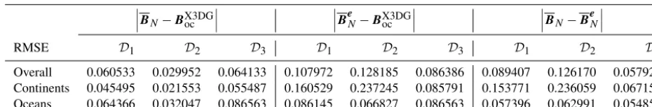
Table 1.Root mean square errors (RMSEs) corresponding to the approximations of the undisturbed forward modelBX3DG_oc as well as the noisy modelBe_oc=BX3DG_oc +ecompared to the “ground truth”BX3DG_oc with the three different dictionaries. Left-hand columns show errors for the approximation ofBX3DG_oc (compare Fig. 7), while center columns show errors for the approximation ofBe_oc(compare Fig. 9). The right-hand columns display the RMSEs of the difference between the respective approximations (as shown in Fig. 10).

BN−B

X3DG oc

B

e

N−BX3DGoc

BN−B

e N

RMSE D₁ D₂ D₃ D₁ D₂ D₃ D₁ D₂ D₃

Overall 0.060533 0.029952 0.064133 0.107972 0.128185 0.086386 0.089407 0.126170 0.057929 Continents 0.045495 0.021553 0.055487 0.160529 0.237245 0.085791 0.153771 0.236059 0.067152 Oceans 0.064366 0.032047 0.086563 0.086145 0.066827 0.086563 0.057396 0.062991 0.054858

reconstruction of the continental noise is even more accurate, while the reconstruction over the oceans only changes very slightly. With the proposed physics-based functions in dic-tionary D3, however, the influence of the continental noise is much less apparent. The maxima occur very close to the coastline, which is most likely due to numerical issues stem-ming from discontinuities of the dataBe_ocin coastal areas. A closer look at the differences|BN−B

e

N|between the approx-imations of noisy and undisturbed data is given in Fig. 10. This shows again that the inclusion of continental noise has a smaller effect on the approximation via physics-based trial functions than on the approximations via the other tested trial functions. Moreover, the corresponding root mean square er-rors of the approximationsBNandB

e

N, respectively, can be found in Table 1. In both cases, we compared the approxima-tions to the undisturbed data BX3DG_oc in order to emphasize the impact of continental noise on the overall approximation. The errors over continental and oceanic regions are provided separately.

4 Conclusions

The main goal of this paper is to study the errors that are made by the approximation of tidal magnetic fields by use of different sets of trial functions. While, e.g., Saynisch et al. (2018) compared forward models for the M2 tidal magnetic field based on different tidal models, we aim at illustrating the effect of the involved trial functions on the possible ex-traction of the tidal magnetic field from satellite data in the first place. The indicated residuals for the synthetic exam-ples show that the use of the presented adapted physics-based trial functions could have a detectable effect for the extrac-tion of such signals in satellite data. These trial funcextrac-tions reflect the underlying physics in the sense that they satisfy the time-harmonic Maxwell equations and that they include knowledge of the ambient core magnetic field and the Earth’s conductivity, but they are not designed to rely on detailed oceanographic models. The latter can be advantageous since the extracted magnetic field induced by ocean tides might eventually be used to make inferences on such models.

Data availability. The authors would like to thank the following providers of software and models: Alexey Kuvshinov for the code of the X3DG solver and a processed version of the depth-integrated tidal ocean velocities from TPXO8-ATLAS, Nils Olsen for the co-efficients of the M2 tidal contribution in the CM5 model, Alain Plat-tner for the code for the generation of vectorial Slepian functions.

Competing interests. The authors declare that they have no conflict of interest.

Special issue statement. This article is part of the special issue “Dynamics and interaction of processes in the Earth and its space environment: the perspective from low Earth orbiting satellites and beyond”. It is not associated with a conference.

Acknowledgements. This work was supported by DFG grant GE 2781/1-1 within the Research Priority Program SPP 1788 “DynamicEarth”.

Edited by: Juergen Kusche

Reviewed by: two anonymous referees

References

Egbert, G. and Erofeeva, S.: Efficient inverse modeling of barotropic ocean tides, J. Atmos. Ocean Tech., 19, 183–204, 2002.

Finlay, C., Olsen, N., and Tøffner-Clausen, L.: DTU candidate field models for IGRF-12 and the CHAOS-5 geomagnetic field model, Earth Planet. Space, 67, 114–130, 2015.

Fischer, D. and Michel, V.: Automatic best-basis selection for geo-physical tomographic inverse problems, Geophys. J. Int., 193, 1291–1299, 2013.

Freeden, W. and Gerhards, C.: Geomathematically Oriented Po-tential Theory, Pure and Applied Mathematics, Chapman & Hall/CRC, 468 pp., 2012.

Recent Progress in Modeling Magnetic and Electric Fields from Sources of Magnetospheric, Ionospheric, and Ocean Origin, Surv. Geophys., 29, 139–186, 2008.

Kuvshinov, A. and Olsen, N.: 3-D Modeling of the Magnetic Fields due to Ocean Tidal Flow, in: Earth Observation with CHAMP, Results from Three Years in Orbit, edited by: Reigber, C., Lühr, H., Schwintzer, P., and Wickert, J., Springer, 2005.

Malin, S.: Separation of Lunar Daily Geomagnetic Variations into Parts of Ionospheric and Oceanic Origin, Geophys. J. R. Astr. Soc., 21, 447–455, 1970.

Michel, V.: Lectures on Constructive Approximation – Fourier, Spline, and Wavelet Methods on the Real Line, the Sphere, and the Ball, Birkhäuser, 2013.

Michel, V. and Telschow, R.: A non-linear approximation method on the sphere, GEM – Int. J. Geomath., 5, 195–224, 2014. Michel, V. and Telschow, R.: The regularized orthogonal functional

matching pursuit for ill-posed inverse problems, SIAM J. Numer. Anal., 54, 262–287, 2016.

Plattner, A. and Simons, F.: Spatiospectral concentration of vec-tor fields on a sphere, Appl. Comp. Harm. Anal., 36, 1–22, https://doi.org/10.1016/j.acha.2012.12.001, 2014.

Sabaka, T., Olsen, N., Tyler, R., and Kuvshinov, A.: CM5, a pre-Swarm comprehensive geomagnetic field model derived from over 12 years of CHAMP, Ørsted, SAC-C and observatory data, Geophys. J. Int., 200, 1596–1626, 2015.

Sabaka, T., Tyler, R., and Olsen, N.: Extracting ocean-generated tidal magnetic signals from Swarm data through satellite gra-diometry, Geophys. Res. Let., 43, 3237–3245, 2016.

Saynisch, J., Irrgang, C., and Thomas, M.: Estimating ocean tide model uncertainties for electromagnetic inversion studies, Ann. Geophys., 36, 1009–1014, https://doi.org/10.5194/angeo-36-1009-2018, 2018.

Schnepf, N., Kuvshinov, A., and Sabaka, T.: Can we probe the con-ductivity of the lithosphere and upper mantle using satellite tidal magnetic signals?, Geophys. Res. Let., 42, 3233–3239, 2015. Simons, F. and Plattner, A.: Scalar and vector Slepian functions,

spherical signal estimation and spectral analysis, in: Handbook of Geomathematics, edited by: Freeden, W., Nashed, M., and Sonar, T., Springer, 2nd Edn., 2015.

Simons, F., Dahlen, F., and Wieczorek, M.: Spatiospectral localiza-tion on a sphere, SIAM Review, 48, 505–536, 2006.