Hydrological Analysis with Respect to Spatial Changes of Urban Growth in Bengaluru City using Geospatial Technology

(1)

International Journal of Innovative Technology and Exploring Engineering (IJITEE) ISSN: 2278-3075, Volume-9 Issue-2, December 2019

Hydrological Analysis with Respect to Spatial

Changes of Urban Growth in Bengaluru City using

Geospatial Technology

Harsh, Birendra Bharti

Abstract— Urban Water Management is the practice of managing freshwater, wastewater, and storm water as components of a basin-wide management plan. It builds on existing water supply and sanitation considerations within an urban settlement by incorporating urban water management within the scope of the entire river basin. The pervasive problems generated by urban development have prompted, in the present work, to study the spatial extent of urbanization in Bengaluru City and patterns of periodic changes in urban development (systematic/random) in order to develop future plans for (i) urbanization promotion areas, and (ii) urbanization control areas. Remote Sensing, using USGS (U.S. Geological Survey) Landsat8 maps, supervised classification of the Urban Sprawl has been done for during 1900 - 2010, specifically after 2000. This Work presents the following: (i) Impact of Land use/cover on ground water level using well location data and (ii) Morphometric analysis of Bengaluru City. The outcome of the study shows drastic growth results in urbanization and depletion of ground water levels in the area that has been discussed briefly. Other relative outcomes like declining trend of rainfall and rise of sand mining in local vicinity has been also discussed. Research on this kind of work will (i) improve water supply and consumption efficiency (ii) Upgrade drinking water quality and wastewater treatment (iii) Increase economic efficiency of services to sustain operations and investments for water, wastewater, and storm water management, and (iv) engage communities to reflect their needs and knowledge for water management.

Keywords— Land Use\Cover change, Buffer Analysis, Uncertainty analysis and Urban Sprawl.

I. INTRODUCTION

The practices of managing freshwater, waste water and storm water are the components of basin-wide management plan which can be termed as urban water management. It builds on existing water supply and sanitation considerations with in an urban settlement by incorporating urban water management within the scope of entire river basin. The consistent increase in the rate of growth of India's urbanization has also facing a big demand for water, as per the various researchers gave their statement that Groundwater potential zone is decreasing due to increase in population or urbanisation.

In 2001, urban population was approximately 285 million and assuming water supply of 135 litres per capita per day, the domestic water requirement is expected at around 38,475 million litres per day (MLD), however as in 2011 urban population was 377 million with a domestic water requirement of 50,895 MLD. It demonstrates that growth in urban population leads to additional water requirement of 12,420 MLD in urban zones.

Revised Manuscript Received on December 05, 2019.

Harsh, M.Tech student, Department of Water Engineering and Management, Central University of Jharkhand, India-835205, Email – [email protected]

Birendra Bharti, Corresponding Author: Assistant professor, Department of Water Engineering and Management, Central University of Jharkhand, India-835205

The water supply of 135 litres per capita per day (LPCD) as a service level, scale should be specified for domestic water use in urban local bodies. However, currently as per the report of Central Public Health and Environmental Engineering Organisation (CPHEEO), an average water supply in urban local bodies is 69.25 LPCD. This indicates that there is a vast gap between the demand and supply of water in urban areas of India.

The problem of access to safe drinking water and sanitation facilities in urban areas of India is also a major concern. It is estimated that by 2050, half of India's population will be living in urban areas and will face acute water problems. At present, 163 million people do not have access to safe drinking-water and 210 million people lack access to developed basic sanitation in India. In urban zones, 96% have access to developed water source capacity and 54% to improved sanitation. Whereas in rural areas, which accounts for 72% of India's population lives, only 84% have access to safe water and only 21% for sanitation. In addition, there is a lack of wastewater treatment facilities to treat the wastewater of a growing population. There is a need to reuse treated wastewater in order to meet the current and future demands for water.

The prevention of pollution of water sources is extremely critical in order to continue to supply water of quality standards. Available data suggests that pollution levels have increased in surface water as well as groundwater. More than 100 million people in urban areas are facing problems of poor water quality. A lack of sufficient infrastructure, services and funds to support water and wastewater treatment facilities required for an urban area further improves the problem. Moreover, the drainage and solid waste collection services are not adequate in most of the urban areas. The systems are poorly planned, designed and managed, or operated with poor maintenance services. As per the use of natural system capacities of soil and vegetation can be useful to absorb and treat waste water.

(2)

Geospatial Technology

The approaches can encompasses in various terms of

managing water related issues, which includes environmental, economic, technical, political as well as various social impacts and implications.

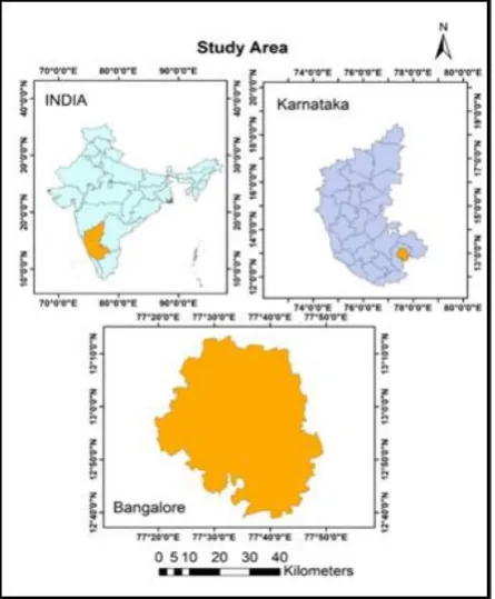
II. STUDY AREA

The problems generated by urban development have prompted, in the present work, to study the spatial extent of urbanization in Bengaluru. It is located in southern India on the largest plateau (Deccan) at an elevation of about 900 m above sea level, which is the highest among India's major cities. It is located at 12.97°N 77.56°E and covers an area of 2117.21 km2.The topology of Bengaluru is horizontal, though the westerly parts of the city are undulating and abrupt. Vidyaranyapura,Doddabettahalli is the highest point, which is 962 metres and is situated to the north-west of the Bengaluru. No vital river run through the city, although the Arkavathi and South Pennar cross tracks at the Nandi Hills, 60 kilometres to the north. Minor tributary of the Arkavathi River i.e. Vrishabhavathi arises within the city at

Basavanagudi and flows through the city. The rivers Arkavathi and Vrishabhavathi together carry much of Bengaluru's sewage. A sewerage system, put up in 2016, covers 215 km2 of the city and connects with five sewage treatment centres located in the periphery of Bengaluru. The larger part number of the city of Bengaluru reclines in the Bengaluru Urban district of Karnataka and the nearby rural areas are a fragment of the Bengaluru Rural district.

[image:2.595.49.272.300.570.2]

Data Collection

Table 1: Data used in Present study

Year Data

Spatial

Source Resoluti

on

201 0

LANDS

AT 8 30m

USGS Earth Explorer (https://earthexplorer.usgs.

gov/)

200 0

LANDS

AT 8 30m

gov/)

199 0

LANDS

AT 8 30m

gov/) 199

0-201

0

Ground water

Data NONE

Central ground water board, Bengaluru (http://cgwb.gov.in) III. METHODOLOGY

Ground Water Data Analysis

After the collection of ground water tube well level data, the data were properly organised. Then latitude and longitude for the ground water stations were located by the use of Google maps, then projected over the study area and verified by superimposing the generated map on Google earth.

Contouring

Contours are basically showing the lines that connect the locations of equal value in a raster dataset which signifies the continuous phenomena such as elevation, temperature, precipitation, pollution, or atmospheric pressure. Basically line features connects the cells of a constant value in the input. Contour lines are often usually stated to as isolines but can also have specific terms depending on what is being measured. Some examples of isobars are pressure, isotherms for temperature, and isohyets for precipitation. The various distributions of the contour lines show the changes in values across the surface area. If there is little or slightly change in a value, the lines are spaced farther separately. If the values rise or drop rapidly, the lines are closer to each other.

IDW (Inverse Distance Weighting)

Inverse distance weighting (IDW) is a form of deterministic approach for multivariate interpolation through a known scattered set of points. The assigned values to unknown points are calculated with a weighted common of the values to be had at the recognised factors.

The call given to this sort of methods become prompted by means of the weighted average carried out, since it motels to the inverse of the gap to each acknowledged point (amount of proximity) after assigning weights.

(3)

Use of this technique assumes the variable being mapped decreases in influence with distance from its sampled place. The Inverse Distance Weighting (IDW) set of rules efficiently is a shifting average interpolator this is typically applied to especially variable records. For positive statistics sorts it's far viable to return to the gathering site and report a new cost that is statistically distinctive from the unique reading but within the fashionable trend for the vicinity. IDW interpolation explicitly implements the assumption that matters which might be near each other are extra alike than the ones which might be farther aside. To expect a value for any unmeasured place, IDW will use the measured values surrounding the prediction region. Those measured values closest to the prediction location could have extra have an impact on at the predicted price than those farther away. Thus, IDW assumes that every measured factor has a neighbourhood influence that diminishes with distance. The IDW function ought to be used whilst the set of factors is dense enough to capture the extent of neighbourhood floor version needed for evaluation. IDW determines cellular values the usage of a linear-weighted combination set of sample factors. It weights the points towards the prediction area greater than those farther away, hence the call inverse distance weighted.

Kriging

In records, in the beginning in geostatistics, kriging or Gaussian technique regression is a technique of interpolation for which the interpolated values are modeled through a Gaussian method governed by means of earlier covariance. Under suitable assumptions on the priors, kriging offers the exceptional linear unbiased prediction of the intermediate values. Interpolating strategies based on other standards including smoothness (e.g., smoothing spline) need now not yield the most possibly intermediate values. The technique is extensively used in the domain of spatial analysis and pc experiments. The technique is also referred to as Wiener–Kolmogorov prediction, after Norbert Wiener and Andrey Kolmogorov.

Ground Water DEM

The most commonplace virtual records of the shape of earth’s floor is mobile-primarily based virtual elevation fashions (DEM’s). This information is used as an input to quantify the traits of the land floor.

Digital elevation models (DEMs) are used to find and manipulate groundwater. This consists of the development of thematic maps from faraway sensing records, topographic maps, hydro-geological information and well data. Thematic maps primarily based on hydro-geomorphology and lineaments must also be organized to higher recognize groundwater assets.

Drainage maps leverage elevation records and are organized from massive scale topographic maps and satellite statistics. Drainage maps play a crucial function in groundwater management.

Methods to analyse spatio-temporal change of Land use/cover

Land Use Land Cover

The terms land use and land cover is often used regularly, but each term has its own significance. Land cover–is the characteristics of Earth’s Surface, and shown by elements like vegetation, water, surface and other physical features

of the land. So characteristics of land cover define the information for activities like thematic mapping and change detection analysis. Land use–shows the activity, economic purpose, intended use, strategy placed on the land cover type by humans. Management practice constitutes land use change. When used together, Land Use / Land Cover shows the classification of different elements on the landscape within a specific time frame based on established methods of analysis of appropriate source data. Land cover is the physical data at the surface of the earth. Land use refers to how people utilize the land for the socio-economic activity, urban use and agricultural land uses are two of the most common high-level classes of use. At any one point or place, there may be a multiple land uses, the specification of which may have a great value. Hence, Land use is the activity for which land is used by the humans. RS & GIS provide efficient methods for systematic analysis of land use and land cover aspects and tools for Land Use/Cover planning and modelling. Satellite data is usually the most used and updated resource available for study the Land Use and land cover which helps in detection of change. Especially with developing towns and cities in India, it is finest method that can show up the urban growth/sprawl. With geographical information system flexible geo-database can be generated for the land use/cover issues. Hence this tool is helpful to bring out the results along with socio–Economic Survey. Knowledge of both land use/cover is important, for planning information on both the above aspects.

Need for Standardization

For recent years, organizations at the different administrative levels have been gathering information about land, yet generally they have worked autonomously and without coordination. Time and again this has implied duplication of exertion, or it has been discovered that information gathered for a particular reason for existing were of practically zero an incentive for a comparative reason just a brief span later. There are a wide range of wellsprings of data on existing area use and land spread and on changes that are happening. Neighbourhood arranging offices utilize point by point data created during ground reviews including specification and perception. Elucidation of enormous scale airborne photos likewise has been utilized generally. Now and again, beneficial data is derived based on utility snare ups, building licenses, and comparable data. Serious issues are available in the application and translation of the current information. These incorporate changes in meanings of classes and information accumulation techniques by source offices, fragmented information inclusion, fluctuating information age, and work of contrary grouping frameworks. What's more, it is almost difficult to total the accessible information in light of the varying arrangement frameworks utilized. Urban regions all epitomize circumstances which must be settled by individual clients and compilers of land use information. The size of the base region which can be delineated as being in a specific land use class depends in part on the scale and goals of the first remote sensor information or other information source from which the land use is recognized and deciphered. It likewise relies upon the size of information

(4)

Geospatial Technology

the land use data. Now and again, land uses can't be related

to the degree of exactness moving toward the size of the littlest unit map capable, while in others, explicit land uses can be distinguished which are too little to even think about being mapped.

Methods for Morphometric Analysis

[image:4.595.309.538.95.258.2]

Evaluation of watershed utilizing quantitative morphometric investigation can give data about the hydrological idea of the stones uncovered inside the watershed. A seepage guide of a bowl gives a dependable file of penetrability of the stones and gives a sign of the yield of the bowl. The DEM has been acquired with a pixel size of 90 m and moreover, it has been utilized to figure slant and angle maps of the watershed. The improvement of waste systems relies upon geography, precipitation separated from exogamic and endogenic powers of the region. Advanced Elevation Model (DEM) information were utilized for getting ready slant, perspective maps and morphometric examination of the watershed. Straight, areal and alleviation parts of the watershed were assessed in GIS condition utilizing Arc GIS programming. Quantitative examination of Orr watershed has been done to assess the waste attributes utilizing GIS programming for estimation and topology working of various morphometric parameters. Important Linear and Arial parameters and their characteristic were calculated such as basin area, perimeter, basin length, bifurcation ratio (Rb), drainage density (Dd), stream frequency (Fs) circulatory ratio (Rc), elongation ratios (Re) from Table II. The drainage patterns of the watershed are dendritic with third order streams.

Table II:- Formula used for computing morphometric parameters

SL.No. Parameters Formulas

1 Stream order (U) Hierarchical rank 2 Stream length (Lu) Length of

stream 3 Mean stream length Lsm=Lu\Nu

4 Stream length ratio RL=Lu\(Lu-1)

5 Bifurcation ratio Rb=Nu\Nu+1 6 Mean bifurcation ratio Rbm=avg. of

bifurcation ratio 7 Drainage density Dd=Lu\A 8 Drainage texture T=Dd X Fs 9 Stream frequency Fs=Nu\A 10 Elongation ratio Re=D\L 11 Circulatory ratio Rc=4PA\P2

12 Form factor Ff=A\L2

13 Relief R=H-h

14 Relief ratio Rf =R\L

IV. RESULT AND DISSCUSSION Ground water data analysis results

The following results was found after the interpolation of dug well points, the interpolation results produced shows temporal change of ground water from 1990, 2000 and 2010.

Fig. 2, show the IDW monsoon in year 1990. The major area have groundwater level <5 meter below ground level(mbgl) and are shown with dark blue colour while lesser area came under >20 mbgl are shown with orange.

Fig. 3, show the IDW pre monsoon of year 1990. The major area have groundwater level in between 10-15 meter below ground-level (mbgl) and are shown with yellow colour while lesser area came under 5-10 mbgl are shown with blue.

Fig. 4, show the Kriging monsoon of year 1990. The major area have groundwater level

[image:4.595.306.529.317.491.2] [image:4.595.60.272.415.727.2] [image:4.595.306.532.549.723.2]

(5)

dark blue colour while lesser area came under >20 mbgl are shown with orange.

Fig. 5, show the Kriging pre monsoon of year 1990. The major area have groundwater level in between 5-10 meter below ground-level (mbgl) and are shown with blue colour while lesser area came under >20 mbgl are shown with orange colour.

Fig. 6, show the IDW monsoon in year 2000. The major area have groundwater level <5 meter below ground level (mbgl) and are shown with dark blue colour while lesser area came under >20 mbgl are shown with orange.

Fig. 7, show the IDW pre monsoon of year 2000. The major area have groundwater level in between 10-15 meter below ground-level (mbgl) and are shown with yellow colour while lesser area came under 5-10 mbgl are shown with blue.

Fig. 8, show the Kriging monsoon of year 2000. The majorarea have groundwater level <5 meter below groundlevel (mbgl) and are shown with dark blue colour while lesser area came under >20 mbgl are shown with orange.

Fig. 9, show the Kriging pre monsoon of year 2000. The major area have groundwater level in between 5-10 meter below ground-level (mbgl) and are shown with blue colour while lesser area came under >20 mbgl are shown with orange colour.

[image:5.595.306.539.50.216.2] [image:5.595.52.284.85.241.2] [image:5.595.306.526.292.447.2] [image:5.595.49.289.298.460.2] [image:5.595.50.282.507.678.2] [image:5.595.307.530.519.673.2]

(6)

Geospatial Technology

Fig. 11, show the IDW pre monsoon of year 2010. The major area have groundwater level in between 15-20 meter below ground-level (mbgl) and are shown with light orange colour while lesser area came under 5-10 mbgl are shown with blue.

[image:6.595.50.267.51.197.2]

Fig. 12, show the Kriging monsoon of year 2010. The major area have groundwater level <5 meter below groundlevel (mbgl) and are shown with dark blue colour while lesser area came under >20 mbgl are shown with orange.

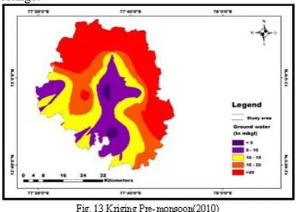
Fig. 13, show the Kriging pre monsoon of year 2010. The major area have groundwater level in between 15-20 meter below ground-level (mbgl) and are shown with light orange colour while lesser area came under >5 mbgl are shown with blue colour.

As per the well location point it was found that Kriging interpolation technique gives a valuable result with respect to IDW interpolation technique in 1990. According to the result, In IDW most of the reason are lies under Less than 5m below ground level, but it is fact that the all areas cannot lies under the same ground level due to change in

slope or elevation of the present study which can be seen in Fig. above. But according to the result of Kriging Interpolation technique, 771.63 Km2 are lies under less than 5m below ground level but in IDW 1842.25 Km2 areas are lies under less than 5m below ground level. 810.61 Km2 are lies in 5-10m below ground level through Kriging method and only 210.75 Km2 are lies in 5-10m below ground level through IDW method.

As per the analysis, from 1990 to 2010 Groundwater level is decreasing above the year, due to huge urbanization and demand of public for various land use. From 1990 to 2000, there is not a very much difference Groundwater level but 1990 to 2010 Groundwater level is decreasing. Due to this, in future the Bengaluru city has facing a huge problem of water.

Spatio-temporal change of land use\cover results From the Table III, Area Classification of Land Use\Cover map we can see how urbanisation has taken place from 1990 to 2010.

TABLE III: Area Classification Of LU/LC

NAME AREA(1990) km2 _{AREA(2000) km}2

ARE A(201 0) km2

FOREST 633.16 454.08

611.9 8

CROPLAND 859.47 871.3

740.7 9

BUILD-UP AREA 344.64 431.28

569.4 5

SHRUBLAND 55.86 38.6 17.56

BARREN LAND 1.94 1.38 0

FALLOW LAND 231.4 335.31

189.9 7

WASTE LAND 1.38 1.38 0

WATER BODIES 55.19 50.01 52.77

[image:6.595.49.270.270.419.2] [image:6.595.47.264.484.638.2]

(7)

Similarly as per this observation, it analysed that Fallow land has showing a good groundwater levelprospect as comparison to others like barren land and built up areas as shown in fig. 14, fig. 15 and fig. 16.

From this comparison the urbanisation of Bengaluru city can be easily analysed from year 1990-2010.

Morphometric Results

From fig. 17 the flow direction has been analysed and it’s found that the surface has maximum slope at the centre of the area.

Total area of the study area was 2117.21km2. Rb bifurcation ratio was 3.49. Generally the value of bifurcation ratio lies between 3-5, the observed value 3.49 shows less structural disturbances and no distortion in drainage pattern.

Circulatory ratio was found to be 0.5 the value of circulatory ratio lies between 0-1, thus the observed value shows that the basin is less elongated and has low discharge of runoff.

The value of Elongation ratio was observed to be 0.84. The range lies between 0.6-1.Thus the observe value shows that the watershed was less elongated in shape. From fig.18 the stream order has been analysed i.e 3rd order.

[image:7.595.49.256.646.773.2]

Form factor observed value was 0.477 which is true as Rf should be less than 0.7. This values shows that the watershed is less circular in shape and the flow will be for longer duration. The observed value of drainage texture was 1.2 , the range generally lies from 2-8. Thus the observed values determines a much coarse structure of drainage, more infiltration capacity and thus resulting in good recharge scenario as shown in Table IV.

TABLE IV :- PARAMETERS VALUES

Bifurcation ratio 3.49

Form Factor(Rf) 0.48

Elongation Ratio(Re) 1.16

Circularity Ratio(Rc) 0.05

Shape Factor(Rs) 2.1

Drainage Feature 1.21

Relief Ratio 5.36

V. CONCLUSIONS

(8)

Geospatial Technology

1. It was evident from time series analysis of hydrological

data that due to urbanisation, Bengaluru’s ground water potential have been decreasing as larger part of the area have ground water level less than 5 meter below ground level in 1990 while it was noticed that the larger part of area have ground water level between 10-15 meter below ground level in 2000 and major declination of ground water potential can be seen in year 2010 i.e. larger area have ground level more than 20 meters below ground level. 2. Total area of the study area was 2117.21km2. Rb bifurcation ratio was 3.49. Generally the value of bifurcation ratio lies between 3-5, the observed value 3.49 shows less structural disturbances and no distortion in drainage pattern. Circulatory ratio was found to be 0.5 the value of circulatory ratio lies between 0-1, thus the observed value shows that the basin is less elongated and has low discharge of runoff. The value of Elongation ratio was observed to be 0.84. The range lies between 0.6-1. Thus the observe value shows that the watershed was less elongated in shape. Form factor observed value was 0.477 which is true as Rf should be less than 0.7. This shows that the watershed was less circular in shape and the flow will be for longer duration. The observed value of drainage texture was 1.2; the range generally lies from 2-8. Thus the observed values determine coarse structure of drainage, more infiltration capacity and resulting in good recharge scenario.

3. It was evident from the Land use\cover change map that Bengaluru city has undergone a rapid urbanisation i.e. 344 km (1990) to 569 km (2010). Waste land and barrel land are two land use cover classes that have shrunk from 2 km2 in 1990 to zero km2 in 2010. It can be interpreted that this area had been utilised to develop build up area. Water bodies show static area coverage from 1990-2010. The area exhibits 59 km2 in 1990 to 50 km2 in 2010. A large area of Bangaluru is covered with forest and crop land i.e. around 1500 km2 in 1990 to 1300 km2 in 2010. Other areas show slight disturbance.

REFERENCES

1. Abdullah, A.Y.M., Masrur, A., Adnan, M.S.G., Baky, Md.AhmedA., Hassan, Q.K., Dewan, A. 2019. Spatio-temporal Patterns of Land Use/Land Cover Change in the Heterogeneous Coastal Region of Bangladesh between 1990 and 2017. Remote Sens. 2019, 11, 790. 2. Ahmed, F., Rao, K.S. 2019. Application of DEM and GIS in Terrain

Analysis: A Case Study of Tuirini River Basin, NE India. Remote sens. 2019, 21,662.

3. Ashaolu, E.D., Olorunfemi, J.F., Ifabiyi, I.P. 2019. Assessing the Spatio-Temporal Pattern of Land Use and Land Cover Changes in Osun Drainage Basin, Nigeria. J. Environ. Geogr. 2019, 12, 41–50. 4. Ashok S. Sangle. 2017. Morphometric Analysis of Watershed of

Sub-drainage of Godavari River in Marathwada, Andrapradesh Region by using Remote Sensing. International Journal of Computer Applications (0975 – 8887) Volume 125 – No.5, September 2017 5. Balakrishna, k.Balakrishna, D.H.B. 2006. Watershed prioritization

based on morphometric analysis of hemavathy basin using remote sensing and geographical information system. Appl. Water Sci. 2006, 6, 5.

6. Banerjee, A., Singh, P., Pratap, K. 2017. Morphometric evaluation of Swarnrekha watershed, Madhya Pradesh, India: an integrated GIS-based approach. Appl. Water Sci. 2017, 7, 1807–1815.

7. Bartakke, V., Golekar, R.B., Baride, M.V., Patil, S.N., Suryawanshi, R.A. 2013. Lineament and Morphometric Analysis for Watershed Development of Tarali River Basin, Western India. Indian J. Environ. 2013, 4, 7.

8. Bastawesy, M.E., Gabr, S., White, K. 1994. Hydrology and geomorphology of the Upper White Nile lakes and their relevance for water resources management in the Nile basin: Hydrological

Modelling Of The White Nile System. Hydrol. Process. 1994, 27, 196–205.

9. Belal, A.A., Moghanm, F.S. 2011. Detecting urban growth using remote sensing and GIS techniques in Al Gharbiya governorate, Egypt. Egypt. J. Remote Sens. Space Sci. 2011 14, 73–79.

10. Brett Hazen. 2015. Lucas: A system for modeling land-use change. IEEE Computational Science and Engineering 2015, 3(1):24 – 35 11. C. Sudhakar Reddy & C. S. Jha. 2012. Assessment and monitoring

of long-term forest cover changes in Odisha using remote sensing and GIS. Environ Monit Assess 2012, 185:4399–4415.

AUTHORS PROFILE

Mr. Harsh, born and brought up in Gonda, India, is has completed his Post Graduate from Central University of Jharkhand, Ranchi with specializations in Water Engineering & Management.