Design of a wireless acquisition system for a digital stethoscope

(1)

University of Southern Queensland

Faculty of Engineering & Surveying

Design of a Wireless Acquisition System for a Digital

Stethoscope

A dissertation submitted by

Justin Miller

in fulfilment of the requirements of

ENG4112 Research Project

towards the degree of

Bachelor of Engineering (Electrical and Electronic Engineering)

(2)

Abstract

The auscultation of the heart with a stethoscope is one of the most common methods employed by physicians to diagnose cardiovascular and respiratory illnesses. Phono-cardiography refers to the technique of acquiring and recording of heart sound signals. The emergence of teleheath and electronic stethoscope technology has opened new op-portunities for rural and regional medical services including the remote screening of heart murmurs.

This dissertation investigates the design and implementation of a wireless data acqui-sition module to capture auscultation sounds from an electronic stethoscope, and sets the foundation for further research into the area of remote auscultation diagnosis and non-invasive techniques for diagnosing abnormalities.

Methods to detect activity in the signal are evaluated for the suppression of ambient noise and adaptive gain control. Several well known noise reduction techniques for signals acquired from a single source are studied and evaluated. A PI controller is developed to control the gain of the input stage to account for attenuation of the heart and respiratory sounds caused by volume effects (i.e. absorption) of the human body.

(3)

University of Southern Queensland

Faculty of Engineering and Surveying

ENG4111/2 Research Project

Limitations of Use

The Council of the University of Southern Queensland, its Faculty of Engineering and Surveying, and the staff of the University of Southern Queensland, do not accept any responsibility for the truth, accuracy or completeness of material contained within or associated with this dissertation.

Persons using all or any part of this material do so at their own risk, and not at the risk of the Council of the University of Southern Queensland, its Faculty of Engineering and Surveying or the staff of the University of Southern Queensland.

This dissertation reports an educational exercise and has no purpose or validity beyond this exercise. The sole purpose of the course pair entitled “Research Project” is to contribute to the overall education within the student’s chosen degree program. This document, the associated hardware, software, drawings, and other material set out in the associated appendices should not be used for any other purpose: if they are so used, it is entirely at the risk of the user.

Prof F Bullen

Dean

(4)

Certification of Dissertation

I certify that the ideas, designs and experimental work, results, analyses and conclusions set out in this dissertation are entirely my own effort, except where otherwise indicated and acknowledged.

I further certify that the work is original and has not been previously submitted for assessment in any other course or institution, except where specifically stated.

Justin Miller

0050027832

Signature

(5)

Acknowledgments

I would like to express my sincere gratitude to Associate Professor John Leis for his guidance and encouragement throughout the course of this project. Due thanks must go to the Faculty of Engineering and Surveying at the University of Southern Queensland for the resourcing of this project.

Last but not least, I would like to thank my wife, Soo Kooi, and my children, Joshua, Theodore and Elizabeth. This project would be impossible without their patience and support.

Justin Miller

University of Southern Queensland

(6)

List of Figures

2.1 The blood flow through the four valves of the heart. Source: Tilkian and

Conover (2001) . . . 5

2.2 The four valves of the heart. Source: Tilkian and Conover (2001) . . . . 6

2.3 Frequencies of common heart and respiratory sounds. Source:Tilkian and Conover (2001) . . . 6

2.4 Attenuation of the human body due to volume effects Source: Kaniuas et al (2005) . . . 13

2.5 Typical Analogue AGC System . . . 13

2.6 Flow chart of subtractive noise suppression algorithm. Source: Boll (1979) 19 3.1 Spectral Entropy Method of Detecting Signal Activity . . . 25

3.2 VAD Test - Energy of a Clean Signal . . . 27

3.3 VAD Test - Entropy of a Clean Signal . . . 27

3.4 VAD Test - Energy of a Signal with Real Ambient Noise . . . 28

3.5 VAD Test - Entropy of a Signal with Real Ambient Noise . . . 28

(14)

LIST OF FIGURES xiii

3.7 VAD Test - Entropy of a Signal with AWGN . . . 29

3.8 Automatic Gain Control Algorithm . . . 30

3.9 Spectral Subtraction . . . 32

3.10 Spectral Subtraction . . . 33

4.1 Hardware System Design . . . 37

4.2 Hardware System Design . . . 38

4.3 Design of Automatic Gain Control Hardware . . . 39

4.4 Frequency Response of Input Stage . . . 40

4.5 Frequency Response of a 2nd Order Butterworth Filter . . . 42

4.6 Frequency Response of a 2nd Order Chebychev Filter . . . 43

4.7 Frequency Response of a 8th Order Butterworth Filter . . . 43

4.8 Pseudo-Ground . . . 46

4.9 Virtual-Ground . . . 46

4.10 BlueSMiRF Gold Bluetooth Modem . . . 50

4.11 Mechanical switch ’bounce’. Source: http://www.labbookpages.co.uk/ . 51 4.12 Hardware de-bouncing circuit . . . 52

5.1 Data flow of host application . . . 55

5.2 Bluetooth Properties in Windows 7 . . . 56

(15)

LIST OF FIGURES xiv

6.2 Completed prototype on prototype board . . . 62

6.3 MPLAB Integrated Development Environment . . . 63

6.4 PicKit 3 In-Circuit Debugger. Source: http://www.microchip.com . . . 63

(16)

List of Tables

3.1 PGA Gain Settings . . . 31

4.1 MCP6S21 Instruction Register . . . 41

4.2 MCP6S21 Gain Register . . . 41

4.3 MCP6S21 Gain Select Bits . . . 41

(17)

Chapter 1

Introduction

The auscultation of the heart with a stethoscope is one of the most common methods employed by physicians to diagnose cardiovascular and respiratory illnesses. With the growing acceptance of teleheath (remote diagnosis) and electronic stethoscope tech-nologies, the acquisition and graphical display of heart and lung sounds may prove to be beneficial for rural and regional medical services.

The benefits of a wireless stethoscope are numerous: Heart and lung sounds can be transferred to a PC, laptop or mobile phone further further analysis without cables. The patient and practitioner are free to move without hindrance and are safe from potentially fatal voltage sources that may be present on a device that is not properly isolated.

Phonocardiography provides a graphical visualisation of auscultation signals, allowing clinical observation of heart sounds that are characterised by frequencies outside the normal range of human hearing (Tilkian and Conover, 2001). The time-frequency analysis of auscultation signals has been proven to be a powerful diagnosis tool for the segmentation of heart and lung sound components and identification of abnormal heart sounds including systolic murmurs and ventricular septal defects.

(18)

1.1 Overview of the Dissertation 2

The purpose of this report is to review background research in the field of signal process-ing when applied to phonocardiographic records. This includes: (i) An understandprocess-ing of the sounds generated by the heart, (ii) methods of controlling the signal gain before it is sampled, (iii) an evaluation of common de-noising techniques and (iv) an evalua-tion of time-frequency transforms for the display of phonocardiographic signals in the time-frequency domain.

1.1

Overview of the Dissertation

This dissertation is organized as follows:

Chapter 2 reviews past and current research in the field of heart sounds and data

acquisition.

Chapter 3 investigates the signal processing aspects of the project.

Chapter 4 discusses the hardware and firmware design of the wireless acquisition

module.

Chapter 5 discusses the software design of the host application.

Chapter 6 discusses the test and implementation stage of the project.

Chapter 7 concludes the dissertation and suggests further work in the area of remote

(19)

Chapter 2

Literature Review

2.1

Introduction

The auscultation of the heart is one of the most common methods employed by physi-cians to diagnose cardiovascular and respiratory illnesses. The most common auscul-tative tool is the stethoscope. An experienced physician can diagnose a wide range of cardiovascular abnormalities including mitral stenosis and systolic murmurs, how-ever many abnormalities are commonly missed due to an inability to apply selective listening to the various components of the heart beat, or a natural inability to detect frequencies outside the normal range of human hearing. Segmentation of the various heart sound components, including components that indicate an abnormality, can be difficult to achieve if they occur simultaneously or close apart (Tilkian and Conover, 2001).

(20)

2.2 Acoustic Properties of the Heart 4

The phonocardiogram also facilitates a screening process to rule out innocent murmurs before referring the patient to a cardiologist for expensive echocardiography.

This review of literature will cover the foundations of bioacustics pertaining to the cardiovascular system, the capture of auscultative signals in a noisy environment and evaluate methods of transforming heart sounds into the time-frequency domain for analysis.

2.2

Acoustic Properties of the Heart

2.2.1 Cardiac Cycle

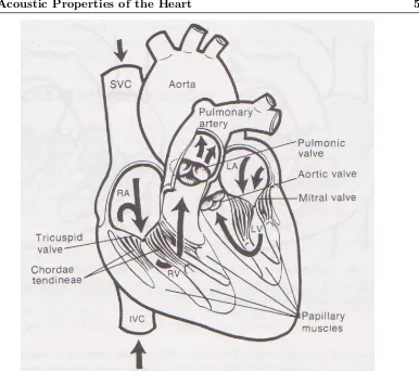
The cardiac cycle can be defined as as the synchronized activity of the atria and the ventricles. During the atrail and ventricular diastole: (i) Venous (deoxygenated) blood enters the right atrium through the superior and inferior venae cavae.(ii) Blood flows into the right ventricle through the tricupsid valve. (iii) Arterial (oxygenated) blood flows from the lung into the left atrium. (iv) The left ventricle is filled with the atrerial blood through the mitral blood (Tilkian and Conover, 2001).

During the atrial systole phase, the atria begins to contract towards the end of the ventricular diastole. During the ventricular systole phase: (i) Venous blood moves through the pulmonary artery from the right ventricle to the lungs for oxidation. (ii) Arterial blood passes through the aorta from the left ventricle to the circulatory system (ibid).

(21)

[image:21.595.138.524.74.417.2]

Figure 2.1: The blood flow through the four valves of the heart. Source: Tilkian and Conover (2001)

2.2.2 Heart Sounds

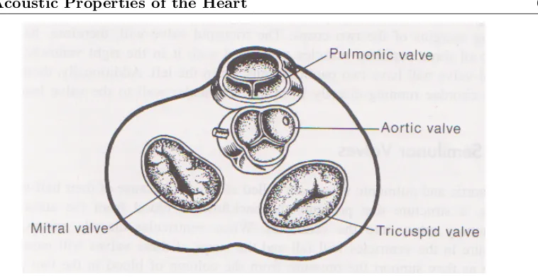
The first heart sound (S1) is caused by the closure of the atrioventricular valves - first the mitral valve followed shortly by the tricuspid valve. The closure of the aortic valve closure, closely followed by the pulmonary valve closure, causes the second heart sound (S2). The first and second heart sounds occur within a frequency range of 20Hz to 175Hz (Tilkian and Conover 2001). Rangayyan and Lehner (1987) however discovered that S1 contained peaks in low frequency range (10-50Hz) and and medium frequency range (50-140Hz), whilst S2 was found to contain peaks in a lower frequency range (10 to 80Hz), medium-frequency range (80-200Hz) and high-frequency range (220-400Hz).

(22)

[image:22.595.141.520.76.271.2]

Figure 2.2: The four valves of the heart. Source: Tilkian and Conover (2001)

and S4 may suggest heart abnormalities, and therefore should be examined carefully (Tilkian and Conover 2001).

Figure 2.3: Frequencies of common heart and respiratory sounds. Source:Tilkian and Conover (2001)

[image:22.595.159.484.361.585.2]

(23)

2.3 Time-Frequency Analysis 7

2.3

Time-Frequency Analysis

Frequency analysis is an important component of phonocardiographic diagnosis. Re-search has found that large intensity murmurs can overlap with the first and second heart sounds (Liang et al, 1997), therefore a time-domain representation of the phono-cardiographic signal alone is inadequate for diagnosis. Analysis of the heart sounds in the frequency domain can be accomplished by performing a Fourier Transform over a segment of the heart sounds.

The Discrete Fourier Transform (DFT) is defined by:

X(k) =

N−1

X

n=0

x(n)ejnωk _(2.1)

where

wk=

2πk N

Time information is lost as a consequence of transforming the signal into the frequency domain. The Fourier Transform is therefore useful for analysing stationary signals (sig-nals that do not vary over time), but inadequate for the study of a signal that contains non-stationary characteristics (Lee et al, 1999). An adaptation of the Fourier Trans-form, the Short-Time Fourier Transform (STFT), computes the time-varying frequency of the signal by calculating the Fourier Transform over a series of short, overlapping segments of the signal (Vikhe et al, 2009). The time information is derived from the location of the current segment (window) under analysis (Lee et al, 1999). To reduce the effects of spectral leakage, each segment is passed through an appropriate window function (Obaidat and Matalgah, 1992).

The Discrete Short-Time Fourier Transform is defined by

X(k, w) =

N−1

X

n=0

w(n−k)x(n)ejnωk _(2.2)

where

wk=

2πk

N (2.3)

(24)

2.3 Time-Frequency Analysis 8

higher frequency components are displayed with equal precision as lower frequency components. Increasing the length of the window will increase the frequency resolution, but at the same time decrease the time resolution of the signal (Obaidat and Matalgah, 1992).

An alternative to the Short-Time Fourier Transform is the Continuous Wavelet Trans-form. Whilst the Fourier transform uses a sinusoidal wave to analyse the signal, the Wavelet Transform transforms a time-domain signal into the time-frequency domain with wavelets of finite energy. Unser and Aldroubi (1996) analogised the wavelet trans-form as a function of correlation of which maximum output occurs when the input signal most resembles the analysis template (mother wavelet).

The mother wavelet is defined by:

ψa,b(t) =

1

√

aψ( t−b

a )dt (2.4)

whereais the scaling parameter and bis the shifting parameter.

The continuous wavelet transform is defined as:

W(a, b) = Z ∞

−∞

x(t)ψa,b(t)dt (2.5)

The time spread is proportional to the scaling parameter a, whereas a is inversely proportional to the frequency. Thus, the wavelet transform exhibits localisation in time whereby higher frequency components are accurately displayed on the time axis.

(25)

2.4 First Heart Sound Detection 9

2.4

First Heart Sound Detection

The observed PCG signal can be modelled as:

S(n) =F(n) +C(n) +N(n) (2.6)

Where F(n) denotes the fundamental components of the heart sound, S1 and S2, C(n) represents a mixture of other heart sound components and N(n) represents noise. The analyse of heart sounds for diagnostic purposes is therefore dependent on adequate segmentation of the heart sound. Accurate segmentation of the heart sounds greatly simplifies the identification of abnormal heart sounds from the cardiac cycle (Wang et al, 2005).

Malarvili et al (2003) demonstrated a simple method of segmenting the heart sound components by correlating the instantaneous energy of the patients ECG signal with the heart sound signal. The segmentation worked under the premise that the opening and closing of cardiac valves are preceded by electrical events of the cardiac cycle.

Iwata et al (1980) introduced a method to detect the first and second heart sounds by spectral analysis. The spectral parameters are extracted from a linear prediction process. An ECG reference is used to aid the selection of the spectral peaks for analysis by limiting the range of tracking .

Since ECG signal analysis is outside the scope of this dissertation, these methods will not be considered.

Liang et al (1997) introduced a time-domain technique of heart sound segmentation that derived an envelope from the Shannon energy principle. The envelope is filtered twice, forward and time-reversed, to remove phase-distortion and delay. After filtering, the signal is normalised to the absolute maximum amplitude of the signal envelope. The average Shannon energy is then calculated over contiguous blocks with the following formula:

Es(t) =

−1

N

X

i=1

(26)

2.4 First Heart Sound Detection 10

Where N is the number of samples in the contiguous block segment.

The average Shannon energy is then normalised with the following equation:

Pa(t) =

Es(t)−E¯s(t)

σ(Es(t)

(2.8)

Where ¯Es(t) and σ(Es(t) is the mean and standard deviation of the average Shannon

energy, respectively.

The output is represented by a series peaks that correspond to the first and second heart sound, other heart sound components, and noise. A threshold is temporarily applied to remove peaks caused by low-level noise. Liang et al added a rule based algorithm to reject extra peaks caused by noise (eg speech) and recover weak heart sound components that are below the threshold. Identification of S1 and S2 follows by identifying the respective systolic and diastolic periods with the assumption that the systolic period is constant whereas the diastolic period is variable.

Liang et al continued their research on heart segmentation by developing an algorithm which used discrete wavelet decomposition and reconstruction to extract the signal within frequency bands that correspond to the first and second heart sounds. The heart sound signal was applied to fifth-level discrete wavelet transform to obtain the 1st to 5th detail coefficients as well as the 4th and 5th approximation coefficients. The signal was reconstructed with a filter bank consisting of 6th order Duabechies filters. The Shannon energy envelogram from Liang et al’s earlier research was applied to the reconstructed detail and approximation frequency bands to determine the peaks that correspond to S1 and S2.

Liang et al argued that the discrete wavelet decomposition and reconstruction method offers greater immunity to previous time-domain and fixed-filter methods. Respira-tion noise was eliminated, however external environmental noise including speech and ambient noise caused errors during segmentation.

(27)

2.5 Heart Rate Detection 11

Wang et al developed an improved segmentation method by implementing a Wavelet de-noising algorithm using prior to reconstructing the coefficients applicable to the S1 and S2 frequency bands. Not unlike Liang’s wavelet segmentation algorithm, the Shannon energy is calculated from the reconstructed signal and analysed to determine the peaks of S1 and S2.

2.5

Heart Rate Detection

A simple approach to determine the heart rate was outlined by Markandey (2009). The heart sound signal is first smoothed by a moving average filter defined by the following expression:

y(i) = 1

N

N−1

X

j=0

x(i+j) (2.9)

Where N is the order of the filter.

The first heart sound is then detected by calculating the maximum slope of the resulting waveform. The heart rate, HR, is calculated as:

HR= fs·60

n (2.10)

Wherefs is the sampling frequency and n is the number of samples between two

con-secutive S1 events.

Markandey’s algorithm applied a moving average to the heart rate to produce a stable heart rate figure suitable for display on a user interface.

2.6

Auto Gain Control

(28)

2.6 Auto Gain Control 12

a power signal-to-noise ratio due to quantisation noise (Young, 1995). Conversely, an AGC can attenuate high-amplitude signals to prevent saturating the ADC (ibid).

With reference to the propose phonocardiogram acquisition module, an input stage consisting of an AGC is necessary because: 1. The output characteristics of the elec-tronic stethoscope are unknown; and; 2. Attenuation of sound due to the volume effects of the human body.

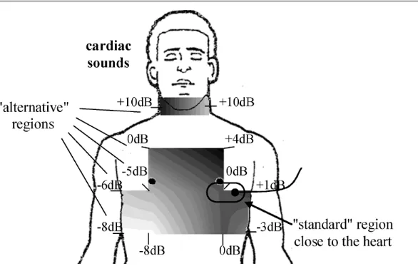
Kaniuas (2006) studied the attenuation of biosignals through the chest region. Volume effects (i.e. absorption) accounted for most of the attenuation, of which the three main causes of sound absorption in the chest were: (i) inner friction, (ii) thermal conduction and (iii) molecular relaxation. Each cause exhibited a different sound absorption coef-ficient. In an earlier paper, Kaniuas et al (2005) demonstrated a correlation between attenuation and the body mass index (BMI). A increased amplitude of auscultative signals were observed in patients with a higher BMI.

Kaniuas approximated the amplitude at the point of auscultation by the following equation:

p(r) =k·p0

r ·e

−α(r)·r _(2.11)

Where k is the constant, r = propagation distance, p0 is the sound pressure amplitude of the point source at r=0, and a(r) is the sound absorption coefficient as a function of r. Kaniuas et al (2005) observed the attenuation at likely regions of the chest to be examined by stethoscope:

It is therefore possible to conclude that a manual gain control would be inadequate for this application because the amplitude of the input signal would vary significantly during the auscultation.

(29)

[image:29.595.184.477.85.275.2]

2.6 Auto Gain Control 13

Figure 2.4: Attenuation of the human body due to volume effects Source: Kaniuas et al (2005)

Figure 2.5: Typical Analogue AGC System

Although Steber noted that analogue AGC systems are low-cost and easily implemented in hardware, Steber identified a number of problems with the analogue AGC system: (i) Analog AGC systems tend to have a poor transient response because of the analogue filter components in the control loop. (ii) Undesirable distortion due to overloading can occur because the gain is a function of average amplitude rather than peak amplitude.

Another constraint, according to Kang and Lidd (1984), is that a gain-change within the analysis window of a time-varying waveform can introduce errors into a system involving analysis and synthesis. This not only creates problem for the de-noising stage of the phonocardiogram acquisition module if a transform/thresholding algorithm is applied to the signal, but also for any subsequent analysis of the heart sounds.

[image:29.595.176.466.334.452.2]

(30)

con-2.6 Auto Gain Control 14

trol system that was equivalent to the analog system. The signal detector was imple-mented by extracting the positive half-cycles from the waveform. If any part of the half-cycle is above the noise-floor threshold, the signal would be multiplied by a gain factor to increase the amplitude of the signal to the maximum value. The noise-floor threshold is pre-determined by the characteristics of the input signal.

Kang and Lidd (1984) introduced a automatic gain control (AGC) algorithm based on a LPC encoder that used low-band energy estimation for voice activity detection. The algorithm used a probably density function to compute the mean value of the low-band energy of the signal to smooth out fluctuations caused by sudden changes in loudness, leakage of higher frequency components and ambient-noise. The error signal of the control loop was calculated by subtracting the mean of the low-band energy from a reference level.The gain would then be incrementally adjusted by an incremental gain with a non-linear relationship to the error.

One of the advantages of Kang and Lidd’s AGC algorithm is that gain is not adjusted during unvoiced (non-speech) periods. Commenting on the auto gain control algorithm, Kang and Lidd noted that steady state was achieved within a few seconds and remained stable with unnecessary gain recalculations.

Archibald (2008) built upon the research of Steber and Kang et al by adding a proportional-integral (PI) controller for detecting voice activity. One distinguishing aspect of Archibald’s auto gain control system is that it incorporates an adaptive noise detection algorithm, whereas the methods proposed by Steber and Kang et al required a LPC encoder to detect speech and non-speech periods. The adaptive noise detection algorithm utilises a PI controller to estimate the noise floor level for voice activity detection.

Stationary noise is determined by computing the variation of signal energy within an envelope. A flat variation indicates stationary noise. In contrast, an envelop with a high variation of signal energy indicates a period of voice/activity. In the event of a non-voice period, the gain is set to 0. Otherwise, the gain is calculated by:

G= DesiredAmplitude

(31)

2.7 Performance Characteristics of Voice Activity Detection 15

Which is a rather simplistic method to correct the gain. On commenting on the pro-posed algorithm, Archibald noted that the quality of the output signal was dependant on the rate of gain change. Audible zipper noise will occur if the gain change is too fast, whereas noise amplification and clipping can occur if the gain change is too slow. This behaviour observed by Archibald corresponds to the transient response of under-damp and over-damped second order systems respectively (Nise, 2000).

Archibald’s algorithm could be improved by applying a proportional-integral-derivative (PID) controller to the amplitude error calculated by:

Error=DesiredAmplitude−P eakAmplitude (2.13)

Ogata (1995) expressed the continuous PID controller as:

m(t) =K

e(t) + 1

Ti

Z t

0

e(t)dt+Td

de(t)

dt

(2.14)

The discrete PID controller can be represented as a difference equation of:

mk=q0ek+q1ek−1+q2ek−2+mk−1 (2.15)

Where coefficients q0 = K

Td

T

, q1 = −K

1 +2Td

T =

T

Ti

and q2 = KT_Td for a

rect-angular approximation of integration. Coefficients q0, q1 and q2 can be determined

experimentally,and/or computed with a maximum descent algorithm (Aigner et al).

2.7

Performance Characteristics of Voice Activity

Detec-tion

Beritelli et al (2002) identified several parameters which characterised the performance of a voice activity detection algorithm:

(32)

2.8 Ambient Noise Cancellation 16

• Mid Speech Clipping (MSC): Clipping due to speech misclassified as noise.

• OVER: Noise interpreted as speech due to a late detection of the transition from active to silence.

• Noise Detected as Speech (NDS): Noise interpreted as speech within a silence period.

To reduce the probability of front end and mid speech clipping from occuring, Woo et al (2000) proposed the formation of a hysteresis based on the estimated noise floor.

2.8

Ambient Noise Cancellation

The quality of heart sounds acquired by a phonographic device can be impaired by internal (bodily) and external noise sources. Leading causes of noise include respiration sounds, movement of the patient, movements of the stethoscope (shear noise) and external environmental noises (Varady, 2001).

Grumet (1993) identified numerous external environmental noise sources in a clini-cal environment. Call buttons, telemetric monitoring systems, electronic intravenous machines, patient-activity monitors and personal movement are typical examples of en-vironmental noises that were identified by Grumet. Grumet measured an average noise level of 67db in acute care admission and general medical wards at night. A study into noise pollution in a hospital setting by Cabrera and Lee (2000) supported this observation in a separate study that found the noise levels in a typical urban hospital would often exceed 55db.

Whilst much of research into noise within a clinical setting focuses on the psycholog-ical impact on patients, the cancellation of ambient noise is of utmost importance to phonocardiography which requires a signal with a relatively high signal to noise ration for accurate analysis and diagnosis (Zhoa, 2005).

(33)

because ambient noise can be caused by various sources at various frequencies and signal intensities (Liang et al , 1997). Another difficulty is presented by the process of selecting the frequency range of the fixed frequency band without degrading the useful heart sounds components in signal (Varady, 2001). A superior de-noising technique would involve the use of an adaptive filter as the impulse response of an adaptive filter is adjusted automatically to operate under changing conditions and minimise the signal error (Widrow et al, 1975).

The Weiner filter is an optimal filtering method that suppresses noise without degrading the useful components of the signal (Widrow et al, 1975). The impulse response of a Weiner filter is designed so that the output closely approximates the characteristics of the expected signal (Proakis and Manolakis, 1996). Consider the following model:

From above model, the error can be mathematically represented as:

e(n) =d(n)−y(n) (2.16)

An ideal filter will reduce the mean-square error to zero.

The FIR Weiner filter of length M can be defined as

y(n) =

M−1

X

k=0

h(k)x(n−k) (2.17)

Whereh(k) represents the coefficients of the filter.

The objective of the Weiner filter is to minimise error. From equation (2.16), the mean square error is :

εM =E|e(n)|2 =E|d(n)−

M−1

X

k=0

(34)

Minimization ofεM yields:

M−1

X

k=0

h(k)γxx(l−k) =γdx(k) (2.19)

Whereγxx is the autocorrelation of the input signal andγdx(k) is the cross-correlation

between the expected and input signals, that isE[d(n)x∗(n−k)] (Proakis and Manolakis, 1996).

Equation (2.19) can be expressed as:

ΓMhM =γd (2.20)

Where ΓMhM is a M x M dimension Toeplitz matrix comprising of the autocorrelation

of the input signal and γd is the cross-correlation vector of the expected and input

signals (Proakis and Manolakis, 1996).

To solve for the optimal filter coefficients, hM:

hM = Γ−M1γd (2.21)

The above equation takes the form of a series of Yule-Walker equations which can be efficiently solved by the Levinson-Durbin algorithm (Proakis and Manolakis, 1996).

One disadvantage of the Wiener filter proposed above, according to Widrow et al (1975), is that it requires a ”priori” knowledge of the expected signal characteristics. However, this information can be recorded in a noise free environment and stored in memory.

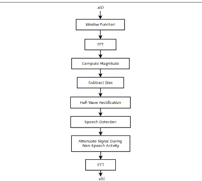
Boll (1979) proposed a subtractive noise suppression algorithm that obtained the noise spectrum during periods of inactivity. The signal is buffered into contiguous frames and windowed to eliminate spectral leakage. The fast Fourier transform (FFT) is applied to the signal and averaged over successive frames. During periods of non-speech activity, the noise floor level, also known as the bias, is estimated.

(35)

[image:35.595.117.525.81.447.2]

Figure 2.6: Flow chart of subtractive noise suppression algorithm. Source: Boll (1979)

magnitude value from three adjacent frames where the magnitude is less than the noise floor level calculated in an earlier step. The signal is attenuated during periods of non-speech activity, and finally transformed back into the time domain with an inverse fast Fourier transform (IFFT) function.

Boll’s spectral subtraction algorithm presents a problem in relation to phonocardio-graphic signals. Heart sounds are non-stationary signals (Iwata, 1980), thus averaging the magnitude may cause temporal smearing of short transitory sounds (Boll, 1979). Scarlat (1996) noted that the power spectral method proposed by Boll produced un-natural artefacts described as ”musical noise”

(36)

2.9 Signal Encoding Techniques 20

applied to perform cross-channel cancellation of noise whereby the wavelet coefficients of the noise reference were subtracted from the wavelet coefficients of the heart sounds. Adaptive thresholding was applied to the resulting coefficients to remove residual noise. The signal is reconstructed with the inverse wavelet transform.

Varady’s algorithm assumes the presence of a second transducer to provide the noise reference, however the noise can be extracted from non-speech (or non-heart beat) sections as demonstrated by Archibald (2008) and Boll (1979).

Zhao (2005) studied a form of wavelet shrinkage that derives the threshold function from the Stein Unbiased Risk Estimate (SURE). The Stein Unbiased Risk Estimate is a statistical function that adaptively optimises the threshold levels used to remove noise from the signal. Zhao’s wavelet shrinkage method makes the assumption that the energy of the useful components will be concentrated in a few coefficients of the wavelet transform, whereas noise will be uniformly distributed. Therefore, Zhao’s algorithm is expected to be effective against ambient environmental noise (eg air conditioning) but not so effective against non-stationary noise such as speech or crying.

2.9

Signal Encoding Techniques

In order to transmit the heart sounds wirelessly, the heart sounds must be encoded in a digital format that is resilient to a high noise environment. The two encoding methods covered in this section are (i) Pulse code modulation (PCM) and (ii) Continuously variable slope delta modulation (CVSD).

Pulse code modulation (PCM) is a common technique for converting analogue signals into a binary code for transmission.The amplitude of each sample is represented by a word of data. A significant disadvantage of PCM encoding is the higher bandwidth requirements compared to single-bit word encodings such as CVSD (Young, 1994). Despite the simplicity of PCM, Prabhu et al (2006) argues that PCM is more prone to interference than CSVD.

(37)

2.10 Conclusions 21

delta modulation. A sample is represented by a single bit which refers to change in the amplitude of the signal. CVSD encoders typically require a higher sample rate due to the reduction of bits per sample (Prabhu et al 2006).

2.10

Conclusions

(38)

Chapter 3

Signal Processing

3.1

Chapter Overview

This chapter reviews fairly important signal processing principles that are applicable to this project. Topics including voice activity detection, automatic gain control and noise reduction will be investigated in this chapter.

3.2

Voice Activity Detection

3.2.1 Introduction

Voice activity detection (VAD) is the process of classifying ”silent” and ”voiced” pe-riods in a signal. In this research project, voice activity detection is applied to signal obtained from a digital stethoscope. Thus, ”voiced” periods refer not to human speech, but rather to auscultation noises (eg heart beats). As ”silent” periods often contain ambient noise, it is possible to perform a spectral estimation of noise during the silent periods. Thus voice activity detection forms an integral component of the noise reduc-tion algorithms discussed later in this chapter.

(39)

3.2 Voice Activity Detection 23

detect activity in a signal, namely:

• Energy Method

• Entropy Method

Each method follows a similar process:

1. Segment the signal into frames of 64. 2. Calculate the energy or entropy of the signal 3. Smooth the value with a moving average. 4. Determine if the value is greater than the estimated noise floor. If it is greater, the segment is a heart sound. If the value is lower than the noise floor, the segment is silence. 5. The noise floor is estimated from the silent segments of the signal.

3.2.2 Energy of Signal Method

Energy is often used as a measure of activity in a signal. A periodic signal over a finite time is said to have high energy, whereas a silent period will have significantly low energy.

The energy of a discrete-time signal can be found by:

E=

N−1

X

i=0

|x(i)|2 _(3.1)

Alternatively, in accordance with Parseval’s Theorem, the energy of a discrete signal may also be found from the frequency domain by:

E= 1PN

N−1

k=0

|X(k)|2 (3.2)

(40)

The standard deviation of signal energy can also be used as a foundation to a VAD algorithm. Segments showing a high degree of standard deviation indicate a periodic signal with significant variation (e.g. a heart beat) The standard deviation of signal energy is calculated by:

E= v u u t

N−1

X

i=0

|x(i)−Emean|2 (3.3)

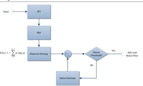
However experimentation with standard deviation method did not indicate any signif-icant performance boosts over the energy method.

3.2.3 Spectral Entropy Method

The entropy of a random sequence is a measure of the unpredictability, or disorgan-isation, of a sequence. A signal consisting of white noise is inherently unpredictable, therefore the entropy is high. The periodic nature of a heart sound is more organ-ised, therefore the entropy approaches zero. This hypothesis can be applied to signal processing for the detection of useful sounds (eg heart sounds) in a noisy signal.

Shannon’s equation to calculate entropy in a sequence is:

E=

N−1

X

i=0

p(i)·log(p(i)) (3.4)

where p is the probability density function (PDF) of a signal.

The PDF can be estimated from the power spectral density (PSD) of the signal:

(3.5)

where X is the fourier transform of the signal.

(41)

[image:41.595.190.493.82.265.2]

Figure 3.1: Spectral Entropy Method of Detecting Signal Activity

3.2.4 Adaptive Thresholding

Noise is seldom constant. The amplitude of noise may change abruptly by simply turning on or turning off an air-conditioner. A robust voice activity detector algorithm must take into account variability of noise. Algorithms with a fixed threshold designed for less noisy environments may incorrectly detect noise as activity when operated in a noisy environment. Conversely, an algorithm designed for noisy environments may detect weak signals as noise. Therefore, the threshold must adapt to the noise levels in any given environment.

The noise threshold is estimated by calculating the entropy of the signal during non-active segments in between heart beats. In the event of a continuous auscultation sound (eg gallop rhythm), the signal is estimated before the stethoscope is applied to the chest and between measurements. The noise threshold is ”smoothed” by a function that is analogous to a PI controller. For the entropy method:

N(t) = (1−0.999)∗E(t) + 0.999∗N(t−1); (3.6)

Where N = noise and E = entropy of the current segment.

(42)

inactivity to activity, and vice versa) to complete before changing state. The hysteresis also provides a degree of tolerance for short variations in entropy during the active and inactive segments.

Setting the range of the hysteresis function is an art in itself. If Ts is too high (re-membering that a high entropy indicates predictability of the signal), each heart sound will be truncated as the amplitude drops below the threshold. However this behaviour occurred rarely during testing, due to the PI behaviour of the threshold estimation al-gorithm. On the other hand, if Tn is set too low, the transition stage from non-activity to activity is detected late, resulting front end clipping (FEC), as defined by Beritelli et al(2002), is introduced.

A signal completely absent from noise will have a noise floor of zero, thus the entire signal will be a ”voiced” segment.

3.2.5 Attenuation of Non-Envelope Segments

To improve the perceptive audio quality of the signal and ultimately increase the signal-to-noise ratio, non-voice (noise only) segments are removed from the signal.

3.2.6 Test Method

The three methods discussed in this section were tested for resiliency to error against 2 test signals as follows:

• Clean normal heart beat signal

• Normal heart beat signal with additive white Gaussian noise

• Normal heart beat signal superimposed with ambient hospital noise

(43)

A small amount of Additive White Gaussian Noise (AWGN) was added to the clean signal to model ambient noise. A real sample acquired from a hospital is then superim-posed with the signal to investigate the performance of the VAD in a real environment.

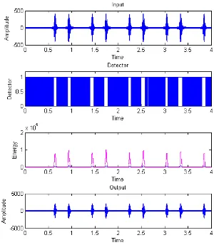
[image:43.595.241.392.220.393.2]

3.2.7 Test Results

Figure 3.2: VAD Test - Energy of a Clean Signal

[image:43.595.240.392.513.683.2]

Figure 3.2 shows the performance of the energy method when applied to a clean signal. As expected, the heart beats are detected as periods of activity.

Figure 3.3: VAD Test - Entropy of a Clean Signal

(44)

[image:44.595.241.391.146.321.2]

active periods. The adaptive threshold is set low due to the absence of ”disorganised” signals, such as white noise.

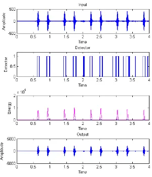
Figure 3.4: VAD Test - Energy of a Signal with Real Ambient Noise

Figure 3.5: VAD Test - Entropy of a Signal with Real Ambient Noise

The performance of the energy and entropy methods for real noise are shown in figures ??and 3.5 respectively. Both methods performance comparitively well.

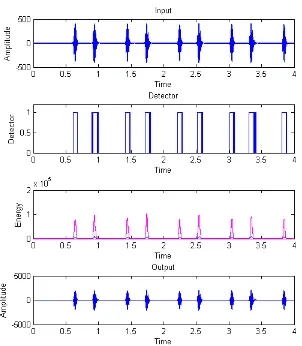
[image:44.595.241.391.381.556.2]

(45)

[image:45.595.240.390.102.274.2]

Figure 3.6: VAD Test - Energy of a Signal with AWGN

Figure 3.7: VAD Test - Entropy of a Signal with AWGN

3.2.8 Conclusion

[image:45.595.241.390.339.508.2]

(46)

3.3 Automatic Gain Control Algorithm 30

3.3

Automatic Gain Control Algorithm

3.3.1 Design

The automatic gain control serves several important purposes, including the follow:

• BMI

• Amplify weak signals

• Attenuate signals to prevent clipping

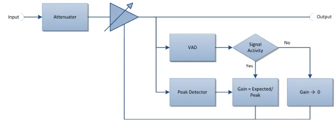
[image:46.595.149.485.371.491.2]

The system design of the auto-gain algorithm proposed for this project is shown in figure??.

Figure 3.8: Automatic Gain Control Algorithm

3.3.2 Programmable Gain Amplifier (PGA) Controller

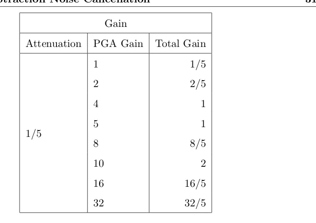
A hardware attenuator divides the input signal by 4. The signal is then applied to the input of a programmable gain amplifier which is controlled by the digital signal controller. The PGA selected for this project will amplify the input signal with a gain of 1, 2, 4, 5, 8, 10, 16 or 32.

(47)

3.4 Spectral Subtraction Noise Cancellation 31

Gain

Attenuation PGA Gain Total Gain

1/5

1 1/5

2 2/5

4 1

5 1

8 8/5

10 2

16 16/5

[image:47.595.202.524.79.307.2]

32 32/5

Table 3.1: PGA Gain Settings

3.3.3 Transition State

To prevent abrupt sudden changes in gain during a transition state, the peak amplitude of the last 16 segments are stored in a sliding window. The maximum value is selected from the sliding window.

3.4

Spectral Subtraction Noise Cancellation

Adaptive Spectral Subtraction, as shown in figure 3.9 involves a statistical analysis of the signal to detect silent periods, of which the spectra of the ambient noise is calculated and stored in memory. During an active period, the FFT of the signal is determined and noise is subtracted. Further thresholding of the signal may be applied at this point. The signal is transformed back to the time domain, ideally in a de-noised state.

To evaluate the performance of the spectral subtraction algorithm, additive White Gaussian Noise was injected into a clean signal. The results are shown in figure 3.10.

(48)

3.5 An Evaluation of Data Communication Protocols 32

Figure 3.9: Spectral Subtraction

is to remove the noise at the host PC instead.

3.5

An Evaluation of Data Communication Protocols

3.5.1 Introduction

(49)

[image:49.595.186.456.97.329.2]

Figure 3.10: Spectral Subtraction

3.5.2 Raw PCM

This approach involved streaming raw PCM, without metadata (eg header), to the desktop PC. The Wave header would be prefixed to the stream for playback on the desktop storage. Data obtained from the 12 ADC was stored in two bytes, hi and low (the 4 highest significant bits were padded with 0s), and streamed to the PC one byte at a time.

This approach preserved the full integrity of the acquired signal, however without a method to synchronise the signal at the host, the stream was often read in the wrong sequence (eg lo byte from the previous packet read as hi, hi packet from the current packet read as lo) if a byte was dropped by the communication link.

3.5.3 Custom Data Structure

DLE, STX, LEN, DATA, DLE, ETX

(50)

If DLE occurred during the data segment, another DLE would be prefixed to the data byte. The length of the packet was included to ensure the data integrity at the other end, since in theory, the frame could be of variable length. If a mismatch was detected, the packet would be dropped by the host and the sequence would be filled with 0s for length N.

The implementation of this method was not immune to error however. The presence of more than two consecutive DLE characters in the signal would cause errors at the receiver end.

3.5.4 uLaw and aLaw

The 12 bit signal would be up-scaled to 16 bit, and then companded to an 8 bit loga-rithmic value. Both standard preserve much of the signal.The benefit of this approach is that the data does not need to be encapsulated in a data packet. i.e. the companded data can be streamed raw. The data is already in a format that can be sent to a remote host via VOIP technology. The disadvantage is the inherent loss in reducing the bit resolution of a sampled signal.

3.5.5 Conclusion

(51)

3.6 Chapter Summary 35

3.6

Chapter Summary

(52)

Chapter 4

Hardware and Firmware Design

4.1

Chapter Overview

This chapter covers the hardware design aspects of the project. A top-down approach was employed to design the circuit: Starting from the system level and ending with the schematics.

4.2

Specifications

The hardware was designed to fulfil the following requirements:

1. The input shall accept line level signals from a digital stethoscope.

2. The acquisition module shall operate from a single voltage source of 3.3V

3. Frequency components less than 1000Hz shall be sampled

4. The signal path shall be protected by galvanic isolation

(53)

4.3 System Design 37

4.3

System Design

4.3.1 Acquisition Module

The system consists of the following modules:

• Input Stage and Automatic Gain Control

• Analogue-To-Digital Converter (including anti-aliasing filter)

• Signal Isolation and power isolation

• Digital Signal Controller

• Bluetooth Modem

Figure 4.1: Hardware System Design

The schematics of the acquisition module are listed in Appendix C.

4.3.2 Receiver

The receiver side, as shown in figure 4.2, consists only of a Bluetooth modem and PC.

(54)

4.4 Automatic Gain Control 38

Figure 4.2: Hardware System Design

4.4

Automatic Gain Control

4.4.1 Input Stage and Fixed Attenuator

The output of the electronic stethoscope is capacitively coupled to the input stage of the wireless module to remove the DC component from the input. This was a necessary compromise because the external signal source references system ground, whereas the acquisition modules operates from a virtual ground referenced at Vdd/2 due to the single-supply operation of the circuit. When a voltage source that is referenced to system ground is connected to a op-amp stage that is referenced to virtual ground, a non-negligible DC offset exists at the input. The presence of this offset is problematic when the input was DC coupled because of the limited dynamic range available to the amplifiers (and analogue-to-digital converter) due to the low-voltage constraints of the circuit.

The solution is to AC couple the input, however this comes at a price. The decoupling capacitor in series with the resistance network of the attenuator forms a high pass filter which is undesirable as heart sounds contain valuable data at very low frequencies. A sufficiently large capacitor is therefore required to preserve as much of the low frequency components of the signal as practically possible. Given a Thevenin equivalent resistance of 1M for the attenuation circuit, a capacitor value of 0.22uF would provide a cut off frequency of 0.723Hz.

(55)

gain is set less than 4, held constant at 4 and amplified at gains greater than 4.

The signal is attenuated by a resistive network and op amp configured to provide an approximate attenuation rate of 1:4 and an input impedance of approximately 1M Ohm. Line level outputs commonly have a very low output impedance (around 6-30 Ohms), therefore loading effects are negligible.

Figure 4.3: Design of Automatic Gain Control Hardware

Due to the low-voltage requirement of this circuit, an op-amp with rail-to-rail amplifi-cation was required to maximise the dynamic range of the circuit. The op-amp selected for this task was the MCP601, a CMOS op-amp especially designed for signal-rail ap-plications.

The attenuator and AC coupled input stage was simulated by MICROCAP, as shown in 4.4.

4.4.2 Programmable Gain Amplifier (PGA)

(56)

Figure 4.4: Frequency Response of Input Stage

instruction.

The PGA can amplify the signal at gains of 1, 2, 4, 5, 8, 10, 16 and 32. Thus, factoring in an approximate attenuation ratio of 1:4, the resulting signal will be attenuated/am-plified by a factor of 0.25, 0.5, 1, 1.25, 2, 2.5, 4 and 8 respectively.

A test point is provided after the PGA for testing and validation.

4.4.3 SPI Interface

The PGA is controlled by a unidirectional SPI bus consisting of the clock, data-in and chip-select lines. Gain is set by first pulling the chip select low. This instructs the device to begin accepting serial data from the SPI bus. The chip-select will remain at the low logic state until the instruction and gain select bytes have been sent.

This is followed by setting the ’Write to Register’ command bit (bit 7) of the instruction register, as shown by table 4.1. All other command bits are set to 0. The resulting instruction byte in hexadecimal is 0x40.

After the instruction register is set, the first (least significant) three bytes of the gain register, as represented by table 4.2, to a value that represents the desired gain.

(57)

Instruction Register

Bit 7 Bit 6 Bit 5 Bit 4 Bit 3 Bit 2 Bit 1 Bit 0

0 1 0 0 0 0 0 0

Table 4.1: MCP6S21 Instruction Register

Gain Register

Bit 7 Bit 6 Bit 5 Bit 4 Bit 3 Bit 2 Bit 1 Bit 0

0 0 0 0 0 X X X

Table 4.2: MCP6S21 Gain Register

Gain

Gain Setting (Decimal) Setting (Binary)

2 0 000

4 1 001

5 2 010

8 3 011

10 4 100

16 5 101

32 6 111

Table 4.3: MCP6S21 Gain Select Bits

Finally, the chip-select is returned to the nominal high logic state to instruct the PGA to process the instruction and gain registers.

The PGA adjusts the gain when the two following conditions are met:

1. A 16 bit word, consisting of the instruction and gain bytes, is fully sent.

(58)

4.5 Data Acquisition 42

4.5

Data Acquisition

4.5.1 Anti-Alias Filter

Elementary Shannon-Nyquist theorem states that the sampling frequency must be at least twice the highest frequency component of the sampled signal. The most common practice is to filter the signal with a low pass filter to remove frequency components above the Shannon-Nyquist frequency.

The first design performed anti-aliasing by a 2nd order low-pass Butterworth filter in a standard Sallen Key topology. The filter was designed with a cut off frequency of 1khz for an expected sampling rate of 2kHz. The frequency response is show in figure 4.5.

However, it was observed that the 2nd order filter did not provide an adequate roll-off for anti-aliasing purposes. As a result, frequencies well above 1kHz were sampled which introduced unwanted artefacts in the discrete signal due to the effects of aliasing.

Figure 4.5: Frequency Response of a 2nd Order Butterworth Filter

The filter was redesigned for a Chebychev response which provided a sharper roll-off than the Butterworth (at the expense of a larger ”ripple” in the passband). This provided only marginal improvement over the Butterworth filter, as seen in figure 4.6.

There were two obvious flaws with the design:

1. The transition region crossed over the Nyquist frequency.

(59)

Figure 4.6: Frequency Response of a 2nd Order Chebychev Filter

The solution was to increase the order of the anti-aliasing filter and increase the sam-pling rate to take into account the non-ideal properties of a low-pass filter (namely, the roll-off within transition region).

The signal-to-noise ratio of an ideal analogue-to-digital converter can be calculated by:

SN R= (1.763 + 6.02b)dB (4.1)

Where b = bit resolution.

An ideal 12 bit ADC will have a SNR of 74db. It is therefore desirable to design a low-pass filter with an attenuation of at least -74db at 1/2 the Nyquist frequency or lower. The final design consisted of an 8 pole Butterworth low-pass filter with a gain of -74db at 2905Hz as shown in figure 4.7. The sampling rate was increased to 8kHz.

Figure 4.7: Frequency Response of a 8th Order Butterworth Filter

(60)

therefore equivalent resistances were constructed with a trim technique as shown by table 4.4.

Resistor Values

Desired R1 R2 Final Resistance Error (%)

9.76 10 390 9.75 0.102

21.5 22 910 21.48 0.090

10.7 12 100 10.71 0.134

15.8 22 56 15.79 0.032

7.68 8.2 120 7.68 0.059

3.65 3.9 56 3.65 0.107

Table 4.4: Trimmed resistor values used by the anti-aliasing filter

4.5.2 ADC

The signal is then sampled by a 12bit ADC and transferred to the microcontroller over the SPI bus. The reference voltage is tied to the Vdd (3.3V) rail so that Vdd/2 becomes the centre point.

4.5.3 SPI Interface

(61)

4.6 Power Supply 45

4.6

Power Supply

4.6.1 Battery Management

The acquisition module was designed to operate on battery. The benefits of battery operation include true wireless functionality and isolation from mains power supply. A rechargeable single cell lithium-ion battery was considered ideal for this application given its superior energy to weight ratios and slow loss of charge when not in use. However the charge process for a lithium-ion batteries requires special monitoring and control, therefore battery management was implemented with the help of the Microchip MCP73812.

4.6.2 Voltage Regulation

The digital signal processor operates on a voltage of 3.3V, whereas the nominal supply voltage is 3.7V when operating from battery or 4.20V when powered by an external power source (eg wall adapter). Regulation is therefore required given a the DSC’s specified maximum voltage of 3.6V. The relatively small margin of 0.4V requires the use of a low drop-out (LDO) regulator.

The MCP1700 satisfies this requirement, providing a stable output voltage of 3.3V with a typical overhead of 178mV. As per conventional linear regulator applications, the input and outputs are bypassed with a capacitor to reduce noise and improve stability of the regulator circuit.

4.6.3 Single Supply Design

(62)

[image:62.595.175.521.81.264.2]

4.6 Power Supply 46

Figure 4.8: Pseudo-Ground

However this circuit is subject to small variances in input voltage, resister drift and mismatches in resistance. A far better option is to reference the the input to a virtual earth which is formed by an unity gain op amp, as shown by 4.9

Figure 4.9: Virtual-Ground

[image:62.595.219.424.369.511.2]

(63)

4.7 Isolation 47

4.7

Isolation

4.7.1 Medical Standards

Roy et al discovered that currents as low as 100 mA can paralyse the respiratory system and cause the heart muscle to fibrillate (1976). Leakage current could originate from the mains earth conductor, from another external device, or from the patient via the applied part.

IEC 60601-1 defines a set of safety standards for electronic medical equipment. IEC 60601-1 standard was adopted by Australia under AS/NZ 3200.1 and may be used to support the electrical safety component of an application to register the device under the Australian Register of Therapeutic Goods (ARTG).

Any medical device that comes into physical contact with a patient is defined by the IEC 60601-1 as an applied part. The diaphragm of an electronic stethoscope is placed against the patient’s chest, often for cardiac diagnosis. As such, an electronic stethoscope is categorised by the IEC as type BF applied part. Type BF medical devices must be separated from the earth to prevent dangerous leakage current flowing through the patient to ground (or vice versa).

Even though the acquisition module is completely isolated from the mains supply (eg powered by battery), there is still the risk of leakage current electrically coupled to the enclosure of the modules that must be mitigated by proper isolation techniques.

4.7.2 Signal Isolation

The IEC 60601 requires medical equipment to withstand an electrical fast transient of 1kV for input/output lines, and up to 2kV protection against surges.

(64)

4.7 Isolation 48

given the non-linear characteristics of opto-coupler and transformer based isolators. The Writer investigated several analogue isolation amplifier solutions available on the market, however none were suitable for a battery powered project (for example, many required dual voltage rails of +/- 15V).

The SPI bus to the ADC and PGA, and the chip select lines, are isolated. Signal isola-tion is provided by the ADUM2400 digital isolator by Analog Devices. The ADUM2400 is fully compliant with the requirements of IEC 60601-1 and is certified for use in med-ical applications.

4.7.3 Power Supply Isolation

Signal path isolation provides little benefit unless the power supply is sufficiently iso-lated. The power supply is isolated by an isolated 3.3V DC-DC converter.

The NKE0303DC is compliant with Underwriters Laboratory (UL) to UL 60950, which specifies an identical distance through isolation (DTI) to IEC 60601. The DTI is the internal-clearance between conductors inside the isolation device. Protection up to 3kV is provided.

The device is a switch-mode converter operating at a typical switching frequency of 115kHz with a specified worse case ripple voltage of 80mV peak to peak. It is therefore necessary to filter the output to reduce the ripple voltage. As recommended by the data sheet, an LC filter was applied to the output in order to attenuate the ripple. The LC notch filter was designed a resonant frequency of 23.215kHz on the premise that the switching frequency of the DC-DC converter would be maintained well above this level. SPICE simulation confirmed that the rippled would drop to 3.9mV.

(65)

4.8 Digital Signal Controller 49

4.8

Digital Signal Controller

A digital signal controller is a variant of traditional microcontrollers that provide barrel shifters and multiply accumulators (MAC) which are used extensively in digital signal processing applications

The first step in the design process was to identify a digital signal controller that fulfilled a set of criteria, including:

• Low voltage (3.0-3.6V)

• UART for communications to the Bluetooth module

• SPI communication module to control the PGA and ADC.

• Low pin count (Desirable, but not mandatory for the prototype)

This narrowed the field down to two microcontrollers: Texas Instruments MSP430 family and Microchip dsPIC33 family. The dsPIC33 was chosen because it offered more RAM, faster processor speed and a hardware USART.

To simplify the circuit design, the microcontroller is clocked by an internal PLL at 80MHz (40 MIPS). An ISCP interface is provided for on-board firmware updates and debugging.

4.9

Bluetooth Modem

(66)

[image:66.595.209.430.90.209.2]

4.10 User Interface 50

Figure 4.10: BlueSMiRF Gold Bluetooth Modem

4.10

User Interface

The user interface was kept simple, consisting only of an LED to display when data capture is in process, and a push button to enable and disable data capture.

Following conventional design principles, current to the LED is supplied by the mi-crocontroller through a current limiting resistor. A GPIO pin was set aside for this purpose.

A simple momentary switch shorts a pull-up resistor to ground when it is pressed. The input pin is mapped to a interrupt which invokes a callback from the interrupt service routine (ISR).

4.10.1 Switch De-bouncing

A common problem with mechanical switches, shown in figure (?), is that the transition between on and off is rarely clean. The conductive contacts ’bounce’ as they are moved to the on or off position. The mechanical oscillations caused by the bounces is also known as as ’switch bounce’.

(67)

[image:67.595.118.525.83.256.2]

4.11 Electromagnetic Compatibility 51

Figure 4.11: Mechanical switch ’bounce’. Source: http://www.labbookpages.co.uk/

To simplify the circuit design and reduce the number of components required, a hard-ware de-bouncing solution was not implement. Instead, a simple softhard-ware de-bouncing algorithm was implemented to filter the transition between on and off.

The interrupt will call the de-bounce algorithm which performs the following:

1. Check the status of the switch input. If the switch input is low, increment the counter. If the switch is high, the switch has bounced - reset the counter.

2. Sleep for 1 millisecond

3. Repeat 10 times

The program will toggle the data capture mode if the input is held for 5 consecutive milliseconds.

4.11

Electromagnetic Compatibility

(68)

[image:68.595.209.432.292.527.2]

4.11 Electromagnetic Compatibility 52

(69)

4.12 Chapter Summary 53

4.12

Chapter Summary

This chapter discussed the hardware design of the acquisition module, including the following topic:

• Input Stage and Automatic Gain Control

• Analogue-To-Digital Converter (including anti-aliasing filter)

• Signal Isolation and power isolation

• Digital Signal Controller

(70)

Chapter 5

Software Design

5.1

Chapter Overview

The wireless acquisition module designed and implemented during this project would not be very useful without a means of receiving the data for further analysis. The software solution discussed in this chapter will capture the auscultation signal from any Bluetooth adapter that supports the RFCOMM protocol, display the signal on the screen and playback the signal to the PC’s sound card.

5.2

System Design

A simplified

5.3

Data Capture

5.3.1 Bluetooth Interface

(71)

[image:71.595.120.489.79.391.2]

con-5.3 Data Capture 55

Figure 5.1: Data flow of host application

nection over the RFCOMM/SPP protocol, as shown by figure 5.2.

This simplifies development considerably, as the service-discovery (SDP) and low level logic-link control are performed by the operating system. Communication with the acquisition module can be achieved by opening a connection to a visualised serial port (eg COM3).

5.3.2 Asynchronous Serial Communication

(72)

[image:72.595.152.526.78.367.2]

5.3 Data Capture 56

Figure 5.2: Bluetooth Properties in Windows 7

When new data arrives, the component buffers the data into a memory stream and raises an event . The data is then transferred into two local FIFO buffers from the memory stream. One buffer is used by the graphing module, while the other is used by the real time sound play back module.

One important design consideration is the need for thread synchronisation when reading and writing to the buffer. If two or more threads attempt to access the same memory space simultaneously, a race condition could occur leading to unpredictable values. One work around is to lock the buffer to prevent other threads from accessing while it is in use.

5.3.3 uLaw to PCM Conversion

(73)

5.4 Realtime Sound Playback 57

retain most of the dynamic range of the original signal. The functionulaw2linearwas ported to C# from Java code originally developed by Sun Microsystems (Now Oracle).

5.4

Realtime Sound Playback

The function private void InitSound() establishes a DirectSound playback device and creates a secondary buffer for double buffering the sound stream. A new thread is created to transfer