Identifying significant contributors to milk production in the absence of the Herd Size Effect

Identifying Significant Contributors to Milk Production

in the Absence of the Herd Size Effect

Daniel Zamykal1, Mike Steele2,3, Don Kerr4 and Janet Chaseling4 1 _{School of Mathematics, Physics and IT, James Cook University, Queensland} 2 _{Faculty of Business, Technology & Sustainable Development, Bond University, Queensland}

3 _{Faculty of Health Science & Medicine, Bond University, Queensland} 4 _{Griffith University, Queensland}

Email: misteele@bond.edu.au

Keywords: Multiple regression, factor analysis, varimax rotation, comparison

EXTENDED ABSTRACT

Prior to the commencement of deregulation from 1 July 2000, the Australian Dairy Research and Development Corporation conducted a large-scale telephone survey of 1826 Australian dairy farms to examine the current on-farm management practices in relation to milk production and farm and farmer demographics. The questionnaire results from the 214 dairy farms in the sub-tropical region of South East Queensland and Northern New South Wales were analysed (Zamykal et al.

2007) to uncover those significant inputs that affect milk production.

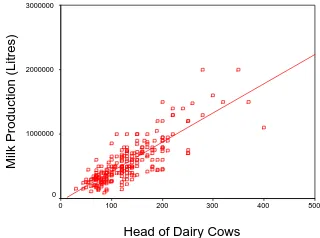
In order to uncover management practices and the underlying but unobservable variables (random quantities) that significantly contribute to milk production, the data was analysed using two major techniques. Firstly, the number of cows a farm possesses is obviously shown to be a significant predictor of milk production (Figure 1).

Head of Dairy Cows

500 400 300 200 100 0

Milk Production (Litres)

3000000

2000000

1000000

0

Figure 1. Plot of milk produced (Litres) against

head of dairy cows. R2 = 0.675.

This strong overriding linear relationship is removed from the analysis by using the residuals from this regression as the new dependent response variable. Therefore, the residuals are the effect of herd size removed or simply the herd size effect (HSE). The original variables are then

regressed against the residuals and the variables which significantly predict the residuals are then highlighted. Secondly, factor analysis was used to extract a reduced number of factors from the sample correlation matrix R, in the absence of the

HSE. It was anticipated that the model derived from the factors would consist of a few interpretable factors that explained some underlying but unobservable random quantities hidden within the original variables. These new factors where then regressed against the residuals derived from the initial regression with the intent of highlighting those significant unobservable random quantities.

Both models produced from the analysis revealed a number of similarities and differences. Comparison of the two linear models reveals that age or experience is negatively associated with predicting milk production in the absence of the HSE. The use of irrigation was also found to be an important component in predicting the residuals. Comparison of other variables and components revealed differences in the composition and interpretability of both models. The factor model allowed the analysts to discover an unobservable random quantity that may influence the inclusion of standard variables in the initial regression model. The inclusion of such a factor allowed the analysts to compare the model derived from standard variables and asses whether both models described the same quantities.

1. INTRODUCTION

Within the Australian rural sector, the Dairy Industry is a major contributor to the national economy by employing over 60 000 people and generating $2 billion dollars annually. However, the industry has undergone significant rationalization in the last 30 years resulting in the steady decline of national dairy operations (DRDC 2001). The combined affect of the reduction in government support and the exposure to market forces has driven the decline in dairy establishments but has fuelled the need to increase the scale of operations (Edwards 2003, ABS 2004).

To build capacity for increased production and to assess the sustainability of the Australian dairy industry, a partnership was formed between the Dairy Research and Development Corporation, National Land and Water Resources Audit, Australian Dairy Farmers Federation and the Australian Dairy Products Federation. This partnership initiated a national survey designed to asses the current on farm practices, production opportunities and attitudes amongst dairy farmers. The project was specifically designed to collect data at the regional and sub-regional level to facilitate local decision making. Data was collected within the eight dairy regions and 21 sub-regions. The survey consisted of approximately 86 questions and was concerned with covering a broad range of issues such as farm demographics, water use efficiency, land use efficiency, fertiliser (nutrient) management, effluent management, soil conservation, biodiversity and the capacity and/or motivation to change current practices.

This paper builds on the evidence that the producers from within the sampled region are from a single milk producing population and are therefore treated as one sample (Zamykal et al.

2007). Analysis of both the current survey results and historical data uncovered the significance of the herd size in predicting milk production (Kerr et al. 1995, Kerr et al. 1998, Zamykal et al. 2007). This study aims to remove the affect of the herd size from the analysis and to uncover significant variables or management practices that would otherwise be over shadowed by such a highly correlated predictive variable. In addition, comparison of the two different regression models may help to uncover or reinforce the inclusion of variables in the predictive models.

2. METHOD

Many research questions are focused on predicting one or more dependent response variables based on a collection of independent predictor variables. These variables are thought to exert some influence over the predicted outcome of the response variable. Regression analyses are a set of statistical techniques that allow a researcher to asses the strength and importance of the relationship between the dependent and independent variables. These techniques can be applied to a data set in which the independent variables are correlated with one another and to varying degrees with the dependent variable(s) (Tabachnick and Fidell 2001). Because of their flexibility, they are helpful in experimental research where for instance, correlation among independent variables is created due to unequal numbers of cases in cells or in observational or survey research that involves manipulated variables (Tabachnick and Fidell 2001). Consequently, the technique is especially useful to the researcher who is interested in real world or complicated problems that cannot be reduced to orthogonal designs in a laboratory.

2.1. Multiple Linear Regression

Multiple linear regression employed in this paper utilises a stepwise selection method to derive the final models. Regression model coefficients are estimated using the least squares method. The least squares approach requires the approximation of the regression coefficients such that the predictions generated by the linear combination of model coefficients and the set of predictor variables minimises the sums of squares of the error vector.

It is standard to assume that the error vector is normally and independently distributed with zero expectation (mean) and constant variance: _{~ (0,} 2₎

N

COVRATIO were used in conjunction to reveal any undue influence.

2.2. Factor Analysis

The basic objective of factor analysis is to determine whether the response variables exhibit patterns of relationships so they can be partitioned into subsets of new variables in which members are highly correlated to one another (Schwartz 1971, Cooper 1983). In effect, if two or more variables measure the same quantity then the variables can be combined and studied together rather than separately (Schwartz 1971). Examination of the correlation matrix revealed a degree of correlation among variables and it was deemed appropriate to investigate the data set using factor analysis. Upon implementation of this method two advantages become immediately apparent to the researcher. Firstly, the joint influence of the most widely different variables can actually be studied. Secondly, factor analysis, like principal component analysis, limits the number variables an individual needs to handle (Schwartz 1971, Johnson 1998, Johnson and Wichern 2002). The main advantage factor analysis has over principal component analysis is the ease of interpretation. These interpretable factors convey the essential information contained in the set of original variables and may highlight the relationship among variables in terms of some underlying but unobservable random quantity (Johnson and Wichern 2002). In this paper, factors were extracted from the sample correlation matrix

R due to the presence of variables with differing

units and variances. The total number of factors extracted from the data set was decided using a combined method of selecting factors with eigenvalues greater than one and the visual assistance of a SCREE plot.

In the event that the original loadings within factors are not readily interpretable, it is usual practice to rotate them until a simple structure is achieved. The rational is akin to focusing the lens on a camera in order to see the detail more clearly. When a varimax rotation is undertaken the analyst has three goals in mind (Lawley and Maxwell 1962). The first one is to reduce the number of negative loadings to a minimum within the factors. Negative loadings can be difficult and awkward to interpret in a meaningful way. Another is to reduce to zero or near zero as many of the loadings as possible so that it reduces the number of variables that need to be interpreted. And thirdly, to concentrate the loadings of variables on different factors so they contrast with each other, this may improve the interpretability of the factors (Lawley and Maxwell 1962). However it must be

emphasised that this simplistic outcome is not always achievable.

Once the factors have been extracted from the sample correlation matrix R, they are then used as

input into a multiple linear regression model for predicting milk output in the absence of the herd size effect.

3. RESULTS

Historically, dairy operations have increased their herd size in order to produce a greater milk yield. In the light of this trend in operational restructuring and evidence presented from quantitative investigations (Kerr et al. 1998, Zamykal et al. 2007), it is of particular interest to remove this affect from statistical models. It is anticipated that other management practices that influence milk production will be revealed once this affect is removed. In order to remove this affect from the analysis a linear model with head of cows as the independent variable and milk production (L) as the dependent variable was produced. The initial linear model revealed that herd size accounts for 67.5 per cent of the variation in milk production (Figure 2).

Head of Dairy Cows

500 400 300 200 100 0

Milk Production (Litres)

3000000

2000000

1000000

0

Figure 2. Plot of milk produced (Litres) against

head of dairy cows. R2 = 0.675.

(V) stocking rate (Table 1). Diagnostic investigations revealed no unusual or influential cases within the data set. Further investigation of the residuals revealed that they are normally distributed and exhibited a constant variance.

Table 1. Unstandardised regression coefficients,

standard errors and cumulative model R2 values for

the residual model based on all producers, n = 214.

Variables contribute significantly to the regression model at α = 0.05.

Model Unstandardised _coefficients Standard _{error value} R2

Money spent on fertilizer

5.23 0.78 0.18

Years of

experience -2325.88 770.57 0.21

Combined measure of supplements

11.35 4.03 0.23

Average use

of irrigation -59670.09 26991.74 0.25

Stocking rate -27400.17 13818.54 0.26

Constant -22438.71 36258.77

Factors were extracted from the sample correlation matrix R in the absence of the HSE with the intent

of reducing the data set and to reveal any unobservable random quantities or driving forces. In total seven (7) factors were extracted from the data set. The extracted factors account for 71.535 per cent of the covariance structure present within the original data set. Once the factors were regressed against the residuals, four significant factors were identified. The significant factors selected were (I) factor seven; (II) factor four; (III) factor five and (IV) factor two (Table 2). Diagnostic investigations into leverage and discrepancy revealed no unusual or influential cases within the data set.

Table 2. Unstandardised regression coefficients,

standard errors and cumulative model R2 values for

the residuals derived from all milk producers, n = 214. Factors contribute significantly to the

regression model at α = 0.05.

Model Unstandardised _coefficients Standard _{error value} R2

Factor 7 44153.38 11861.30 0.054

Factor 4 -42605.51 11816.09 0.105

Factor 5 34790.03 11858.43 0.140

Factor 2 25692.82 11766.95 0.159

Constant -5177.54 11826.42

4. DISCUSSION

Removal of the dominant linear trend from the analysis revealed that five variables and four factors are additively significant for the prediction of milk production in the absence of the herd size effect.

Multiple linear regression models using standard variables highlighted the importance of money an operator spends on fertiliser. The inclusion of this variable in the model is unsurprising as pasture growing season has long been linked to milk production (Reid 1990). Any enhancement to the speed of pasture growth will likely have a positive affect on milk production. However, the variables ‘years of experience’, ‘average irrigation usage’ and ‘stocking rate’ have negative coefficients and are negatively associated with milk production in the absence of the HSE.

regime significantly predicts the production of milk yield in the absence of the HSE.

When comparing the variables/factors directly between models it appears that there are differences and similarities in the conclusions that can be drawn from the models. When comparing the first variable in both models, slightly different conclusions can be made. The model utilising standard variables includes the ‘money spent on fertiliser’ as the strongest predictor of the residuals. In the factor regression, factor seven consists of this variable together with other variables that appear to describe a wealth component. This shifts the focus from the application of fertiliser to the ability to spend on fertiliser, supplements and the value of the property itself. This appears to be validated with the inclusion of factor five in the model which appears to be describing the application of fertiliser and not the amount spent. Further comparison of the two linear models reveals that age or experience is negatively associated with predicting milk production in the absence of the HSE. In a study of cost efficiency in the United States dairy industry, Tauer and Mishra (2006) revealed that farmer age increased unit cost of production. This was attributed to the fact that older farmers were less efficient in their management practices (Tauer and Mishra 2006). Lastly, irrigation appears in both models as a significant additive component for predicting milk yield. However, in the initial model, the ‘average use of irrigation’ negatively affects milk production while in the factor model, irrigation positively affects production. Upon closer inspection of the factor loading matrix, factor two loads heavily upon the irrigation variable ‘above average use of irrigation’. Therefore, the models may indicate that an ‘average’ user of irrigation may have a negative affect on production while an ‘above average’ user of irrigation will have a positive affect on production. Unsurprising as diary operators must maintain a pasture growing season in excess of nine months per year to remain viable (Reid 1990).

5. CONCLUSIONS

Identification of the significant variables/factors for the prediction of milk production can be achieved using multiple linear regression models. The inclusion of factors in multiple linear regression models may facilitate the interpretability of unobservable driving forces that would otherwise be overlooked. Factor analysis is a useful tool for uncovering unobservable random quantities that influence the production of milk

within the sample. When directly compared to the model derived from the original variables a different perspective could be gained as to the inclusion and importance of significant variables in the linear regression models. Clearly the factor analysis has not improved the r-squared in the regression and for this reason and its complexity, the standard regression is satisfactory.

6. REFERENCES

ABS. 2004. Year Book Australia 2004. (Australian Bureau of Statistics) Canberra.

Belsley, D. A., E. Kuh, and R. E. Welsch. 1980. Regression Diagnostics: Identifying Influential Data and Sources of Collinearity John Wiley and Sons Brisbane

Cooper, J. C. B. 1983. Factor Analysis: An Overview. The American Statistician

37:141-147.

DRDC. 2001. Sustaining our Natural Resources - Dairying for Tomorrow. Dairy Research and Development Corporation, Melbourne, Australia

Edwards, G. 2003. The story of deregulation in the dairy industry. The Australian Journal of Agricultural and Resource Economics

47:75-98.

Fox, J. 1991. Regression Diagnostics Sage Publications London

Fox, J. 1997. Applied Regression Analysis, Linear Models and Related Methods Sage Publications, London.

Johnson, D. E. 1998. Applied Multivariate Methods for Data Analysts. Duxbury Press, South Melbourne.

Johnson, R. A., and D. W. Wichern. 2002. Applied Multivariate Statistical Analysis, 5 edition. Prentice Hall, Sydney.

Kerr, D. V., J. Chaseling, G. D. Chopping, T. M. Davison, and G. Busby. 1998. A study of the effect of inputs on level of production of dairy farms in Queensland - a comparative analysis of survey data. Australian Journal of Experimental Agriculture 38:419-425

Kerr, D. V., T. M. Davison, R. T. Cowan, and J. Chaseling. 1995. Factors affecting productivity on dairy farms in tropical and sub-tropical environments Asian Australasian Journal of Animal Science

8:505-513.

Lawley, D. N., and A. E. Maxwell. 1962. Factor Analysis as a Statistical Method. The Statistician 12:209-229.

Reid, R. L. 1990. The Manual of Australian Agriculture Fifth edition. Macarthur Press, Brisbane

Schwartz, R. D. 1971. Operational Techniques of a Factor Analysis Model. The American Statistician 25:38-42.

Tabachnick, B. G., and L. S. Fidell. 2001. Using Multivariate Statistics Fourth edition. Allyn and Bacon Sydney

Tauer, L. W., and A. K. Mishra. 2006. Dairy farm cost efficiency. Journal of Dairy Science

89:4937-4943.

Zamykal, D., M. Steele, D. V. Kerr, and J. Chaseling. 2007. Best Management Strategies for the Australian Dairy Industry Using Multiple Linear Regression Techniques in Towards