Extremely low-overhead security for wireless sensor networks: Algorithms and implementation

Rochester Institute of Technology

RIT Scholar Works

Theses Thesis/Dissertation Collections

5-1-2009

Extremely low-overhead security for wireless sensor

networks: Algorithms and implementation

Michael Schab

Follow this and additional works at:http://scholarworks.rit.edu/theses

This Thesis is brought to you for free and open access by the Thesis/Dissertation Collections at RIT Scholar Works. It has been accepted for inclusion in Theses by an authorized administrator of RIT Scholar Works. For more information, please [email protected].

Recommended Citation

Extremely Low-overhead Security for Wireless Sensor

Networks: Algorithms and Implementation

By

Michael William Schab

A Thesis Submitted in Partial Fulfillment of the Requirements for the Degree of Master of Science in Computer Engineering

Supervised by Dr. Marcin Lukowiak

Department of Computer Engineering Kate Gleason College of Engineering

Rochester Institute of Technology Rochester, NY

May, 2009

Approved By:

_____________________________________________ ___________ ___

Dr. Marcin Lukowiak

Primary Advisor – R.I.T. Dept. of Computer Engineering

_ __ ___________________________________ _________ _____

Dr. Shanchieh Jay Yang

Secondary Advisor – R.I.T. Dept. of Computer Engineering

_____________________________________________ ______________

Dr. Manuel Lopez

Thesis Release Permission Form

Rochester Institute of Technology

Kate Gleason College of Engineering

Title: Extremely Low-overhead Security for Wireless Sensor Networks:

Algorithms and Implementation

I, Michael William Schab, hereby grant permission to the Wallace Memorial Library to reproduce my thesis in whole or part.

_________________________________ Michael William Schab

Dedication

Acknowledgements

I would like to thank my RIT committee members, Dr. Lukowiak, Dr. Lopez and Dr. Yang for their advice and guidance in making this thesis a success. Additional gratitude is extended to Dr. Hu for the initial concept of this thesis.

Abstract

Recent advances in the development of compact microprocessors have brought forth new applications in the field of data acquisition and wireless communication. One of these applications is a compact sensor mote that has the ability to perform both data acquisition and transmission within a Wireless Sensor Network (WSN). Wireless sensor communication is susceptible to the same data security threats as traditional wireless networks. In an environment where sensors are broadcasting battlefield intelligence or patient biometrics, data confidentiality must be enforced utilizing some form of encryption.

Unlike traditional wireless networks, where the communicating devices have unrestricted access to power and memory, a wireless sensor has very limited resources. A wireless sensor consists of a battery designed to last an extended amount of time, therefore it is critical that the computation and transmission overhead involved in enforcing data security be optimized to preserve battery life.

Table of Contents

Thesis Release Permission Form ii

Dedication iii Acknowledgements iv

Abstract v

List of Figures viii

List of Tables ix

List of Tables ix

Glossary x Glossary x

1 Introduction 1

1.1 Private Key Cryptography 1

1.2 Public Key Cryptography 1

1.3 Security on Resource Constrained Devices 4

1.4 Related Work 5

1.5 Thesis Objectives 5

1.6 Organization 6

2 Elliptic Curves 6

2.1 Elliptic Curve Groups over Real Numbers 6

2.2 Point Addition for Points with Different x-Coordinates 7 2.3 Point Addition for Points with the Same x-Coordinates 8

2.4 Point Doubling (F + F = 2F, Fy ≠ 0) 9

2.5 Point Doubling (F + F = 2F, Fy = 0) 10

2.6 Point Multiplication 11

2.7 Elliptic curves Groups Over Fp 12

2.8 Point Addition Point Doubling 13

3 Elliptic Curve Cryptography (ECC) 13

3.1 Key Generation 13

3.1.1 Private Key(s) 14

3.1.2 Public Key 14

3.2 Encryption 14

3.3 Decryption 15

4 NTRUEncrypt Implementation 15

4.1 Background 16

4.2 Modulo Arithmetic 18

4.2.1 Modulo of Negative Numbers 19

4.3 Key Generation 20

4.3.1 Private Key(s) 22

4.3.2 Almost Inverse Algorithm 23

4.3.3 Public Key 28

4.4 Encryption 30

4.5 Decryption 32

4.6 Decryption Failures 34

4.7 Why Decryption Works 36

5.1 Star Multiplication 38

5.2 Karatsuba 39

5.3 Karatsuba Multiplication 39

5.4 Recursive Karatsuba (KM) 40

5.5 KM Performance 42

5.6 Private Key Polynomial fp 44

6 Evaluation and Performance 46

6.1 Hardware 46

6.2 Software 48

6.3 Test Setup 49

6.4 ECIES-160 Results 49

6.5 NTRUEncrypt-251 Implementation and Results 52

6.6 NTRUEncyrpt-251 vs. ECIES-160 55

6.7 NTRUEncyrpt-107 56

6.8 Energy Consumption 59

6.8.1 Microprocessor Power Consumption 59

6.8.2 Transmit and Receive Power 60

6.9 Code Size 61

7 Conclusion and Future Work 64

List of Figures

Figure 2.1: Degenerate Curve ... 7

Figure 2.2: Elliptic Curve Point Addition When F ≠ -G... 8

Figure 2.3: Elliptic Curve Point Addition when F = -F... 9

Figure 2.4: Elliptic Curve Point Doubling when F + F = 2F, Fy≠ 0... 10

Figure 2.5: Elliptic Curve Point Doubling when F + F = 2F, Fy = 0 ... 11

Figure 2.6: Elliptic curve Point Addition for Fp... 13

Figure 4.1: Number line representing positive and negative modulo... 19

Figure 4.2: Flow chart from encrypted ciphertext e to plaintext c... 37

Figure 5.1: KM Example ... 42

Figure 5.2: KM polynomial Count [] and Size (N) for each iteration for N=107... 43

Figure 6.1:Crossbow MICAz... 47

Figure 6.2: Crossbow MIB520 Gateway ... 47

Figure 6.3: Actual ECIES-160 Execution Times... 50

Figure 6.4: Actual ECIES-160 Execution Times Including Private Key Generation... 52

Figure 6.5: NTRUEncrypt-251 Average Exec Time for 10 Rounds with CutOff = 252.. 54

Figure 6.6: NTRUEncrypt-251 and ECIES-160 Execution Times... 55

Figure 6.7: NTRUEncrypt-107 Average Exec Times for 10 Rounds with CutOff = 28.. 56

Figure 6.8: NTRUEncrypt-107 Execution Times with Zero Check Enabled... 57

Figure 6.9: NTRUEncrypt-107 Execution Times with Zero Check Disabled... 58

Figure 6.10: ECIES-160 Code Size ... 62

List of Tables

Table 4.1: k = 1 Round of AIA... 25

Table 4.2: k = 2 Round of AIA... 25

Table 4.3: k = 3 Round of AIA... 26

Table 4.4: k = 4 Round of AIA... 26

Table 4.5: k = 5 Round of AIA... 26

Table 4.6: Binary to trinary conversion ... 31

Table 4.7: Trinary to binary conversion ... 34

Table 5.1: KM execution time versus CutOff value ... 44

Table 6.1: MICAz (MPR2400CA) Hardware Specification... 48

Table 6.2 Liu et al vs. my work timing results for ECIES-160 ... 51

Table 6.3: NTRUEncrypt parameter selection based on security... 52

Table 6.4: NTRUEncrypt-251 Execution Times ... 55

Table 6.5: Power Consumption for ECIES-160 and NTRUEncrypt-251... 59

Table 6.6: Public Key Size for NTRUEncrypt-251 and ECIES-160... 60

Table 6.7: Transmit and Receive Power Based on Cryptosystem ... 60

Glossary

ECC Elliptic Curve Cryptography

ECDH Elliptic Curve Diffie Hellman

ECDSA Elliptic Curve Digital Signature Algorithm

ECIES Elliptic Curve Integrated Encryption Scheme

PKCS Public Key Crypto-System

1 Introduction

Security within a network, either wired or wireless, typically involves the use of cryptography. Cryptography is the process that allows for secure communication over insecure channels [1]. A channel is a transport mechanism that facilitates the exchange of information from one location to another using a physical wire or through the air. In order for two parties to communicate securely, they must utilize a mathematically common element, know as a key, to transform and thereby disguise messages being transmitted be each other. The transformation of an intelligible message, called plaintext, into an unintelligible form, called ciphertext, is called encryption. The reverse process of converting the ciphertext back into a usable plaintext form is known as decryption. Whether the key is kept secret among the communicating parties, or a subset of the key is publically shared, defines the type of cryptosystem.

1.1

Private Key Cryptography

A cryptosystem in which the key is ‘shared’ and kept private between the communicating parties is known as a symmetric, or private key, cryptosystem. Since the key is used in both the encryption and decryption process, it must remain private otherwise the security between the two parties will be compromised. As long as a secure channel exists within the private key cryptosystem, private keys can be easily updated on a regular cadence to prevent an adversary from studying the cryptosystem and determining the private key [1].

1.2

Public Key Cryptography

means of a secure channel, thereby allowing anyone to communicate securely to the owner of the public key.

Though public key cryptosystems (PKCS) allow for quick and easy setup, their key size, number of bits, are typically larger than those of a private key cryptosystem of equivalent security level [46]. The public key cryptosystem, RSA [3] whose name was derived from the authors’ initials, has a 1024-bit public key version with an equivalent symmetric security level of only 80-bits [47].

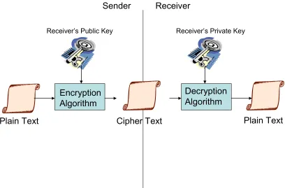
Since the PKCS keys are larger and more complex to create, the amount of computation power required for encryption and decryption is significantly greater than that of a private key cryptosystem. Figure 1.1 provides a high level overview of the process involved in sending an unsecure plaintext message from a sender, the conversion into an encrypted ciphertext, to the final decryption back to plaintext form that a recipient can understand. This is a one way function starting at the sender and ending at the receiver, therefore in order for a message to return back to the sender, the sender would have to provide their own public key to the receiver and the whole process would run in reverse.

Cipher Text Encryption

Algorithm

Decryption Algorithm

Plain Text Plain Text

Sender Receiver

Receiver’s Private Key Receiver’s Public Key

Advantages of Public Key Cryptosystems in Key Distribution

The small key size and low computational complexity of private key cryptosystems allow for fast execution times and low memory usage, but the inherent design of the cryptosystem does not facilitate updating the private key used between the two communicating parties.

Key distribution schemes allow for the secure deployment, or replacement, of the private keys being utilized in a cryptographic system. Secure distribution of these keys between the interested parties typically falls into one of three schemes: Key Distribution Center Scheme, Key Pre-distribution Scheme and Public Key Scheme [29].

The Key Distribution Center Scheme utilizes a central server in which each node interested in communicating on the network must access in order to obtain a private key. In a wireless environment, where nodes are placed in remote areas that rely on message hopping, access to a central server is not an option.

The Key Pre-distribution Scheme involves embedding keys within each node prior to deployment [29]. This can be a universal key or multiple keys stored within each sensor. The universal key, though not requiring much memory space, would easily compromise the security of the network if an adversary were to capture the node and obtain the common network key. Having each node contain multiple keys, a unique key pair per node, reduces the probably of an adversary determining the correct ‘active’ key, however, storing multiple keys per node increases memory size. In a wireless sensor network, such as a battle field, where node counts could be substantial, storing unique keys for per node communication is impractical [18].

1.3

Security on Resource Constrained Devices

Wireless Sensor Network (WSN) applications range from sensors collecting battle field intelligence, to the monitoring of patient vitals such as heart rate and blood pressure. Transmission of confidential data, such as sensitive medical information must be protected from fraudulent activities such as alterations to treatment procedures or drug dosages [5].

Wireless devices within a WSN typically have limited resources including battery life, memory size and processing power. Maximizing battery life is extremely important in environments where sensors are deployed only once and never serviced again. Though transmission and reception of information usually requires the most energy in a WSN [34], the extra processing cycles imposed by an encryption scheme can actually consume more power than communication [9]. Every effort should be directed towards optimization of the cryptosystem code to reduce power consumption.

Data security in resource constrained devices, such as wireless sensors, has traditionally been solved using private key cryptosystems such as MiniSec [6] and TinySec [7]. These private-key based cryptosystems are popular due to their low energy consumption and fast execution times, but sacrifice security. An alternative cryptosystem that provides enhanced security at the expense of increased computational complexity is the asymmetric, or public key, cryptosystem.

NTRUEncrypt is a relatively new PKCS that suggests faster execution times and requires less memory, for an equivalent security level, than ECC and RSA [24]. Conceived in 1996, NTRUEncrypt is a latticed based PCKS that features short, easily created keys with fast execution times and low memory requirements [2].

1.4

Related Work

Challa et al work comparing NTRUEncrypt to RSA clearly shows NTRUEncrypt to have significant performance gains over RSA [16]. Investigation into research benchmarking NTRUEncrypt, to the very comparable ECC cryptosystem, is close to non existent. The closest example by Driessen et al [15], provides an excellent comparison between the NTRUEncrypt based key signature algorithm, NTRUSign, and the comparable ECC equivalent Elliptic Curve Digital Signature Algorithm (ECDSA). Driessen et al research supported their statement of “NTRUSign is superior to the other signature schemes when comparing signature generation and verification time” [15]. Much of the performance gains of NTRUSign were from use of trinary polynomials and Karatsuba [40] variants to obtain a 9x performance increase over ECDSA [15].

A different approach, by Buchmann et al [14], that enhances the performance of NTRUEncrypt’s fundamental operation of polynomial multiplication, involves finding bit patterns within polynomials [14]. By identifying repeating bit patterns, the number of additions required to compute the product of two polynomials can be reduced, thereby lowering execution time.

1.5

Thesis Objectives

depth understanding of the steps involved in the implementation of NTRUEncrypt and how its performance relates to ECIES.

The rationale to compare NTRUEncrypt with ECIES was based on several publications by Challa et al [16] and Wang et al [5] that showed ECC based PKCS to have greater performance than that of RSA [3]. Since ECC based PKCS are very popular in the resource constrained embedded microprocessor market, comparing ECIES to NTRUEncrypt on a resource constrained device was chosen.

1.6

Organization

The remainder of this thesis provides an overview of elliptic curves in Section 2 including the theory involved in the ECIES PKCS. Section 3 introduces NTRUEncrypt and provides a detailed explanation, including examples, of how to implement NTRUEncrypt. Section 4 provides data obtained from an actual implementation of both NTRUEncrypt and ECIES on a wireless sensor, including execution time, RAM and ROM size, and power consumption. Software implementation details, along with Karatsuba optimization techniques used by other researchers, of NTRUEncrypt are discussed. Section 5 concludes this thesis by providing a summary of findings along with suggestions for future work.

2 Elliptic Curves

2.1

Elliptic Curve Groups over Real Numbers

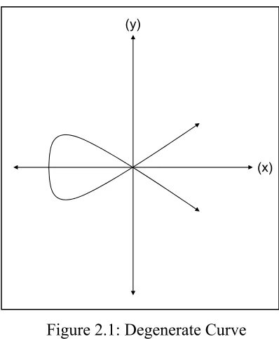
An elliptic curve is a smooth graph that does not contain any self-intersecting points along its curve. Elliptic curves can be used to define a group given the following form with a, b, x and y all being real numbers [8].

b ax x

y2 = 3 + + ₍₁₎

0 27

4_a3 _{+ b}2 _{≠ (2)}

Over a number field, a cubic, i.e. a polynomial of degree three, can have at most three roots, where a root is defined as a point where the curve crosses the x-axis. For real numbers, the roots of a cubic fall into two categories, degenerate and non-degenerate. A degenerate case occurs if any two roots of the cubic coincide with one another, such as the case where the two curve cross at the x-y intersection as shown in Figure 2.1 below:

Figure 2.1: Degenerate Curve

The following examples cover several non-degenerate curve applications.

2.2

Point Addition for Points with Different x-Coordinates

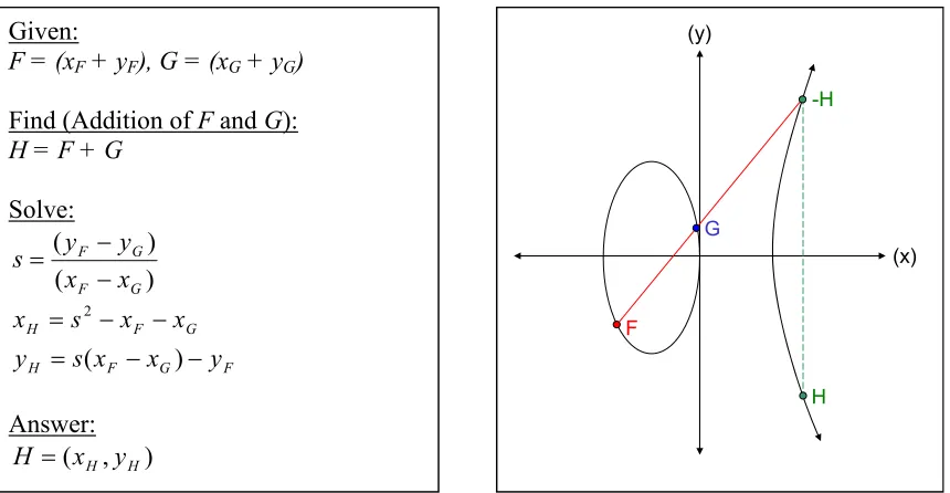
The addition of two points on an elliptic curve can be represented both mathematically, as well as, graphically. The addition of two points, F and G, for points with different x-coordinates, is performed by drawing a straight line through points F and G until the line intersects the curve at a third point –H, because the slope of such line is finite. The next step is to take the reflection of point –H across the x-axis to obtain H. The resultant H is the summation of F and G, see [8].

Figure 2.2: Elliptic Curve Point Addition When F ≠ -G

2.3

Point Addition for Points with the Same x-Coordinates

In this case, the previous point addition technique is invalid. The drawing of a line through these two points results in a vertical line intersecting only two points on the elliptic curve, instead of three. In this case, the elliptic curve group defines a third, infinity point O, with the two points having additive inverses, see[8].

Given:

F = (xF + yF), G = (xG + yG)

Find (Addition of F and G): H = F + G

Solve: ) ( ) ( G F G F x x y y s − − = G F H s x x

x = 2 − −

F G F

H s x x y

y = ( − )−

Figure 2.3: Elliptic Curve Point Addition when F = -F

2.4

Point Doubling (F + F = 2F, F

≠

0)

Doubling of a point involves adding a point to itself. The process involves drawing a line through point F, tangent to the elliptic curve. The line will intersect a second point, -H, on the elliptic curve if Fy ≠ 0. The reflection of point -H across the x-axis results in the product point H, see [8].

Note: If Fy= 0, then the result of doubling F is the infinity point O, see [8].

Given:

F = (xF + yF), G = -F = -(xF + yF)

Find (Addition of F and -F): H = F + (-F)

Answer:

H = F + (-F) = O

-F

F

Figure 2.4: Elliptic Curve Point Doubling when F + F = 2F, Fy≠ 0

2.5

Point Doubling (F + F = 2F, F

= 0)

When attempting to double a point where the y-coordinate = 0, i.e. Fy = 0, the tangent line to the elliptic curve will never intersect a second point on the curve. The tangent line to the elliptic curve is actually vertical and results in the product, 2F, equaling the infinity point O, see [8]. In this example, there are three possible points for F where Fy= 0. Given:

F = (xF + yF)

Find (2F): H = 2F = F + F

Solve: ) 2 (

) 3

( 2

F F

y a x

s= +

Note: a represents one of the domain parameters for the elliptic curve.

H H s x

x ₌ 2₋2

) ( _{F H}

F

H y s x x

y =− + −

Answer: ) , (x_H y_H H =

-H

H

(x) (y)

Figure 2.5: Elliptic Curve Point Doubling when F + F = 2F, Fy = 0

2.6

Point Multiplication

Point multiplication on an elliptic curve utilizes a scalar parameter k multiplied by a point F on the elliptic curve, such that kF = H. Using the previous techniques of point addition and doubling, point multiplication is possible. The following example illustrates the technique [8].

Given k = 17 and point F, find H = kF.

H = kF = 17F = 2(2(2(2F)))) + F

Note: If Fy = 0 for point F, the following substitutions are made in the above equation based on the point doubling equation, Figure 2.5, when Fy= 0.

Given 2F = O, then 2F + F = 3F = F. Continuation of this pattern reveals:

H = kF = 4F = 3F + F = O, 5F = 4F + F = F,….etc

In summary, if scalar k is even, H = O, otherwise H = F.

Given: F = (xF + yF)

Find (2F): H = 2F = F + F

Answer:

H = 2F = O, since Fy = O H3

(x) (y)

2.7

Elliptic curves Groups Over F

Cryptographic use of elliptic curves requires a finite field Fp instead of real numbers. Extending the definition of the elliptic curve from real numbers to a finite field of integers restricts the field size to p values through the use of modulo arithmetic. For an elliptic curve, E(Fp) all computations in Fp are reduced modulo p, therefore an elliptic curve containing non negative integer variables a, b, x and y can be defined as follows [32]:

) (mod

3

2 _{x ax b p}

y ≡ + + (3)

Just as with elliptic curves over real numbers must not contain repeated factors, elliptic curves over a finite field Fp must also maintain this property.

0 ) (mod 27

4_a3 _{+ b}2 _{p ≠ (4)}

Elliptic curves, Fp, consist of a finite number of points thereby making them suitable for cryptosystems. In order to utilize a Fp for cryptography, equation (4) must be satisfied for randomly selected values of a, b, and p.

The following illustrates this step given randomly chosen variables a = 4, b = 3 and p = 5:

) (mod

3

2 _{x ax b p}

y ≡ + +

) 5 (mod 3 4 3

2 _{≡x + x+}

y

Selecting point (2, 4):

) 5 (mod 3 ) 2 ( 5 2 ) 5 (mod

42 _≡ 3 _{+ +}

) 5 (mod 3 10 8 ) 5 (mod

16 ≡ + +

1 1≡

Since point (2, 4) satisfies the equation, it is a valid point on the elliptic curve F5 and can be used for cryptography.

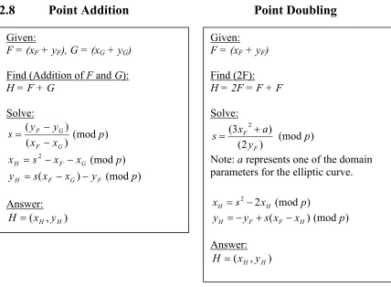
are the same except a reduction modulo p is performed [8]. There is a point addition and point doubling algorithm described as follows.

2.8

Point Addition

Point Doubling

Figure 2.6: Elliptic curve Point Addition for Fp

3 Elliptic Curve Cryptography (ECC)

Elliptic Curve Cryptography (ECC) was introduced by Neal Koblitz and Victor Miller in 1985 [33] and is an accepted standard by IEEE under 1363-2000 & 1363a-2004 with security based on the difficulty of solving the discrete logarithm problem [8]. ECC utilizes a finite group composed of points (x, y) located on an elliptic curve with the encryption and decryption process based on the aforementioned point addition and multiplication.

3.1

Key Generation

ECC key generation starts by selecting a finite field elliptic curve E(Fp) based on Equation (3). Given an elliptic curve E over a finite field Fp, let G be a point that has a

Given:

F = (xF + yF), G = (xG + yG)

Find (Addition of F and G): H = F + G

Solve: ) ( ) ( G F G F x x y y s − −

= (modp)

G F H s x x

x = 2 − − _(modp)

F G F

H s x x y

y = ( − )− (modp)

Answer:

) , (x_H y_H H =

Given: F = (xF + yF)

Find (2F): H = 2F = F + F

Solve: ) 2 ( ) 3 ( 2 F F y a x

s= + (modp)

Note: a represents one of the domain parameters for the elliptic curve.

H H s x

x ₌ 2₋2 _(modp)

) ( _{F H}

F

H y s x x

y =− + − (modp)

Answer:

prime order n within E(Fp). These values can be used to generate cyclic subgroup E(Fp), see [33]:

{G} = {∞, G, 2G,…(n-1)G}

3.1.1Private Key(s)

The private key is an integer k that is selected at random from the interval [1, n-1]. 3.1.2Public Key

The public key, Q, is the private key k, multiplied by a random point H selected from the elliptic curve.

Q = kH (5)

3.2

Encryption

Encryption in ECC starts with the desired plaintext message to send, m. The message, m, is converted into a point, M, in the finite field Fp and is encrypted by adding it to a randomly selected integer k multiplied by the recipient’s public key Q, such that:

E1 = M + kQ (6)

In addition to E1, the sender also calculates E2 by multiplying the previously selected k with the random point H, such that:

E2 = kH (7)

The sender then transmits both point E1 and E2 to the recipient [33]. In order for the recipient to decode the ciphertext points, the two communicating parties must agree on a set of domain parameters, T, that are exchanged up front. The parameters contain a list of 6 items that relate the ciphertext to the original plaintext. The domain parameters are:

Where:

p – Size of field F

a – First value defining curve b – Second value defining curve G – Initial base point on curve n – Order of point G

h - Cofactor

3.3

Decryption

To recover the original message, m, the recipient first must find point M on the elliptic curve given the following equation:

M = E1 – kQ (8)

Utilizing the domain parameters, p, E, H and n, the following substitutions are performed [33].

kQ = k(dG) = d(kG) = d(E2) (9)

Substitution of variables from (9) into (8) results in the following decryption equation for point M.

M = E1 – d(E2) (10)

Since the domain parameters are public, the recipient can reconstruct the elliptic curve and locate the original message, m, given point M.

4 NTRUEncrypt Implementation

NesC [28] is a variant of the C Programming Language that is optimized to run on resource constrained devices.

Pseudo-code representing the actual nesC code developed in this thesis are represented as ‘Algorithms’ throughout the rest of this thesis unless otherwise noted.

4.1

Background

NTRUEncrypt, also known as the NTRU encryption algorithm, is a new PKCS relative to other cryptosystems and was just recently adopted into the IEEE P1363.1™/D12 [22] draft standard for PKCS in February of 2009. NTRUEncrypt was proposed by Hoffstein, Pipher and Silverman in 1996 and is based on ring theory [2]. Security of the cryptosystem relies on the difficulty of finding extremely short vectors within a lattice. It was developed in an effort to provide an efficient public key cryptosystem that required less system resources such as memory and CPU processing power, while still maintaining similar security to that of other PKCS. While the exact translation for the acronym NTRU is not exactly known, several rumored translations include “Number Theorists aRe Us” [1] and “N-Th Degree Truncated Polynomial Ring”.

NTRUEncrypt is based on a ‘Ring of Truncated Polynomials’ represented by ring R below: ) 1 ( ] [ − = _N X X Z

R (11)

The polynomials within the ring, R, consist of all truncated polynomials of degree N-1 having integer coefficients [31].

( )

1 2 2 1 1 0 0 1 0 ... ₋ − − = + + + = ∈

=

∑

N i

N

i

iX R a X a X a X a X

a X

a (12)

) ...( ) ( ) ( ) ( ) ( ) ( 1 1 1 1 1 1 1 1 0 0 0 0 1 0 − − − − − = + + + + + = ∈ + = ⊕

∑

Since the resultant of any polynomial manipulation must remain within R, convolution multiplication of polynomials, or ‘star multiplication’, denoted by the symbol ‘⊗’, is performed the traditional way with the exception that the exponents must never exceed N. Constraining the polynomial to size N is accomplished by reducing and rotating exponents (i mod N).

1 1 2 2 1 1 0 0 1 mod0 ... ) * ( ) ( ) ( ₋ − ₋ − − ≡ + = + + + = ∈ =

⊗

∑

N N N N N n j i n i i i

iX bX R c X cX c X c X

a X

b X

a (14)

Constraining the polynomials to size N has an added benefit when implementing NTRU in software and/or hardware. Unlike traditional multiplication where two N sized polynomials multiplied together could potentially expand to 2N -1 in size, star multiplication limits the size to N, thereby requiring less memory.

The fundamentals of NTRUEncrypt are based on parameters N, p, and q. As mentioned above, N represents the number of degrees of the polynomial ring R. The parameters p and q represent the modulus values used throughout the encryption and decryption process. Both of these modulus values must maintain the following properties [2].

- The gcd(p, q) = 1, i.e. p and q must be relatively prime - The value of q must be considerably larger than p

4.2

Modulo Arithmetic

Modulo arithmetic is a fundamental reduction operation used in many steps of the NTRUEncrypt algorithm. Modulo reduction, referred to as ‘mod’, is the remainder value produced by the division of two numbers [44].

Given: a = 23, b = 7 Find: c = 23 mod 7

2 3

7 23

remainder =

23 mod 7 = 2 The general expression for modulo is:

a mod b

The concept of congruence can be also defined using modulo: a ≡ c(mod b)

With congruency, given a constant b, the value c remains the same regardless of the value chosen for a. The following two values of 23 and 30 are considered congruent to each other.

23 ≡ 2(mod 7) 30 ≡ 2(mod 7)

If a and b have no common factors between them, then it is possible to find an inverse for a(mod b), such that [44]:

a * c ≡ 1 (mod b) Find the inverse of 2(mod 7):

11 * 2 ≡ 1 (mod 7)

4.2.1Modulo of Negative Numbers

Modulo is defined as the difference between the largest integer multiple of the divisor that is less than the dividend. Modulo reduction of a positive number is straightforward:

23 mod 7 = 2

Modulo reduction of a negative number can be difficult to comprehend: -23 mod 7 = 5

The confusion begins with the natural tendency to divide and transfer the ‘sign’ to the quotient. For the example of -23 mod 7, the largest integer divisor less than the dividend is -28, not -23. The number line in Figure 4.1 represents the graphical representation for both -23 mod 7 and 23 mod 7.

Figure 4.1: Number line representing positive and negative modulo

Understanding the concept of negative modulo is extremely important in the implementation of NTRUEncrypt since the private key polynomials contain negative coefficients. The incorrect usage of modulo reduction for negative numbers will result in unexpected polynomial coefficients throughout the NTRUEncrypt algorithm.

The modulo operator ‘%’ in nesC, as well as other programming languages, simply transfers the ‘sign’ value of the dividend to the quotient, thereby resulting in an incorrect solution. As a result, a custom modulo function detailed in Algorithm 4.1, written in nesC, was used to correct this issue.

0

10

20

30

-30

-20

-10

23

21

2 = 23 mod 7

-23

-28

Minor optimizations to prevent the modulo ‘%’ operation from occurring on values equal to zero or less than the ‘modVal’ where added in steps 1 and 3 of Algorithm 4.2.1.

4.3

Key Generation

Key generation in NTRU, just like all asymmetric cryptosystems, creates a private and public key pair. Generation of the private and public keys in NTRU begins with the selection of two polynomials f and g within ring R with coefficients being small relative to the large modulus q. Selection of the two polynomials f and g are constrained to the following criteria:

- Polynomial f must be invertible modulus of both p and q. More specifically [2]:

) (mod 1

) (mod 1

p f

f

q f

f

p q

≡ ⊗

≡ ⊗

(15)

- Polynomial f must contain df number of coefficients equal to ‘+1’, df-1 number of coefficients equal to ‘-1’ and the remaining N-2df -1

coefficients equal to ‘0’. Input: value – Input to apply modulo

modValue – Modulo value to apply Output: Modulo reduced value

Init: retVal = value 1: If ( value = 0 ) 2: Return 0

3: If ( retVal + modVal <= 0 OR retVal – modVal >= 0) 4: retVal = value % modVal

5: If ( retVal < 0 )

6: retVal = retVal + modval 7: Return retVal

- Polynomial g must contain dg number of coefficients equal to ‘+1’, dg number of coefficients equal to ‘-1’ and the remaining N-2dg coefficients equal to ‘0’.

- To ensure security, generation of both polynomials f and g, need to be random generated by means of a Random Number Generator (RNG) or Index Generation Function (IGF) detailed in [22].

Note: The reason df contains an unequal number of ‘+1’ and ‘-1’, is due to the constraint of fto be invertible, since a polynomial f(1) = 0 can never be inverted. Polynomial g does not need to be invertible and therefore has an equal number of ‘+1’s to ‘-1’s [2].

Since the only requirement to generate a random polynomial is an input count for the number of ‘+1’ and ‘-1’, Algorithm 4.2 loops through an n sized polynomial, inserting num_ones count of ‘+1’ or num_neg_ones count of ‘-1’ at random positions.

4.3.1Private Key(s)

NTRUEncrypt requires the generation and storage of two private keys, f and fp. The generation of the private key polynomial f utilizes Algorithm 4.2 with df number of‘+1’ and (df -1) number of ‘-1’.

The second private polynomial key, fp, is the inverse calculation of f modulo p (f mod p). Calculation of this inverse, in the ring of truncated polynomials R, is performed using either the Extended Euclidean Algorithm (EEA) [22] or the Almost Inverse

Input: n – Nth degree size of polynomial

num_ones – Number of coefficients equal to ‘+1’ num_neg_ones – Number of coefficients equal to ‘-1’

Output: a(x) = Polynomial with random coefficients equal to -1, 0, or +1

Init: pos = 0

1: While ( num_ones OR num_neg_ones ) {

2: rVal = RandomNumberGenerator 3: pos = rVal % n

4: if (num_ones AND a(pos) = 0) {

5: a(pos) = 1;

6: num_ones = num_ones - 1 }

7: rVal = RandomNumberGenerator 8: pos = rVal % n

9: if (num_neg_ones AND a(pos) = 0) {

10: a(pos) = -1

11: num_neg_ones = num_neg_ones - 1 }

}

Algorithm (AIA) [19]. Wilhelm’s investigation into the performance of both algorithms suggests the AIA to have better performance and therefore was utilized in this thesis [23]. 4.3.2Almost Inverse Algorithm

By definition, a polynomial b is invertible, modulo p, if the resultant inverted polynomial B maintains the following property [31].

) 1 (mod ) (mod

1 −

=

⊗_{B p x}N

b (16)

The work in presented by Silverman et al [20] presents two AIA implementations, one for modulo p = 2 and another for modulo p = 3. The combined AIA, Algorithm 4.3, was written to support both modulo reductions thereby reducing code space. The specific changes required to add p = 2 support to the base p = 3 algorithm are shown as bolded

Input: a(x) – Polynomial to invert n – Nth degree size of polynomial

c – Modulo value to apply to coefficients

Output: b(x) ≡ a(x)-1 – Inverse polynomial of a(x) in (Z/cZ)[x] / xn – 1; NoInverse; or ERROR

Init: k = 0, b(x) = 1, c(x) = 0, f(x) = a(x), g(x) = xn – 1 Error Check: If (c != 2 OR c != 3)

Return ERROR

1: Loop: {

2: While ( f(0) = 0 AND NumDegrees( f(x) != 0 ) ) {

3: f(x) = x

x f( ) 4: c(x) = c(x)⊗x 5: k = k + 1 }

6a: If ( NumDegrees( f(x) ) = 0 ) {

6b: If ( f(x) = 1 OR ( f(x) = -1 AND c = 3 ) ) 7a: Return f(0)x(n – k) ⊗b(x) (mod xn-1)

Else

7b: Return NoInverse;

}

8: If ( NumDegrees( f(x) ) < NumDegrees( g(x) ) ) {

9: Swap f(x) & g(x) 10: Swap b(x) & c(x) }

10a: If ( c = 3 AND ( f(0) = g(0) ) ) {

11: f(x) = f(x) - g(x) (mod c) 12: b(x) = b(x) - c(x) (mod c) }

ELSE {

13: f(x) = f(x) + g(x) (mod c) 14: b(x) = b(x) + c(x) (mod c)

}

To demonstrate the property of inversion, an example detailing the process involved in finding the inverse of polynomial b using the AIA, Algorithm 4.3, is shown.

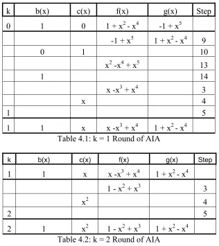
Given: N = 5, p = 3, b = 1 + x2 – x4 Find: B = b-1

Tables 4.1-4.5, illustrate the number of ‘rounds’ required to find the inverse of b = 1 + x2 – x4. A ‘round’ is characterized by the variable k and is incremented whenever the conditional f(0) = 0 is satisfied for polynomial f(x) (Step 2 of Algorithm 4.3). Each column is labeled with the variable name referenced in the AIA Algorithm 4.3, with the column labeled ‘Step’ corresponding to the particular operation step in the algorithm. The first entry in Table 4.1 is the initial setup as shown in the ‘Init’ section of Algorithm 4.3.

k b(x) c(x) f(x) g(x) Step

0 1 0 1 + x2 - x4 -1 + x5 -1 + x5 1 + x2 - x4 9

0 1 10

x2 -x4 + x5 13

1 14

x -x3 + x4 3

x 4

1 5

1 1 x x -x3 + x4 1 + x2 - x4 Table 4.1: k = 1 Round of AIA

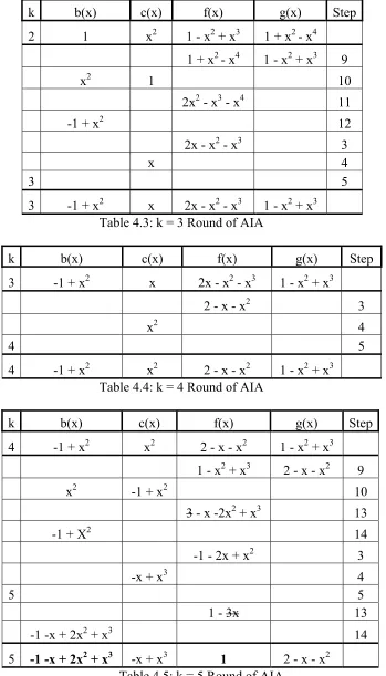
k b(x) c(x) f(x) g(x) Step

1 1 x x -x3 + x4 1 + x2 - x4

1 - x2 + x3 3

x2 4

2 5

k b(x) c(x) f(x) g(x) Step 2 1 x2 1 - x2 + x3 1 + x2 - x4

1 + x2 - x4 1 - x2 + x3 9

x2 1 10

2x2 - x3 - x4 11

-1 + x2 12

2x - x2 - x3 3

x 4

3 5

3 -1 + x2 x 2x - x2 - x3 1 - x2 + x3 Table 4.3: k = 3 Round of AIA

k b(x) c(x) f(x) g(x) Step

3 -1 + x2 _{x 2x - x}2 _{- x}3 _{1 - x}2 _{+ x}3

2 - x - x2 3

x2 4

4 5

4 -1 + x2 x2 2 - x - x2 1 - x2 + x3 Table 4.4: k = 4 Round of AIA

k b(x) c(x) f(x) g(x) Step

4 -1 + x2 x2 2 - x - x2 1 - x2 + x3

1 - x2 + x3 2 - x - x2 9

x2 -1 + x2 10

3 - x -2x2 + x3 13

-1 + X2 ₁₄

-1 - 2x + x2 3

-x + x3 4

5 5

1 - 3x 13

-1 -x + 2x2 + x3 14

The effects of modulo reduction throughout the AIA can be observed in Step 13 of Table 4.5. After the ‘Addition’ Step 13, the coefficient 3 was reduced to zero thereby decreasing the polynomial by one degree.

Algorithm 4.3 continues to increment variable k until the number of degrees of f(x) = 0 (Step 6a). Step 6b is evaluated next and is responsible for determining whether or not the polynomial is actually invertible. If f(x) != ± 1, Algorithm 4.3 is aborted and returns a value indicating no inverse exists (Step 7b). If an inverse is found, i.e. f(x) = ± 1, Step 7a is executed to reveal the inverted polynomial B as follows:

) 1 (mod ) ( ) 0 ( ( ) _{⊗ −}

= _{f x} n−k _{b x x}n

B (Step 7a of Algorithm 4.3)

) 1 (mod ) 2 1 ( ) 1

( (5 5) _{⊗ − − +} 2 ₊ 3 5 ₋

= _x − _{x x x x}

B ) 1 (mod ) 2 1 ( ) 1 )( 1

( _{⊗ − − +} 2 ₊ 3 5 ₋

= x x x x

B

3 2 2

1 x x x

B=− − + + (Inverse polynomial)

As a final check for inversion, Equation (16) is used to verify polynomial B is the inverse polynomial of b.

) 1 (mod ) (mod 1 − =

⊗_{B p x}N

b ) 1 (mod ) 3 (mod 1 ) 2 1 ( ) 1

( _+x2 _−x4 _{⊗ − −x+ x}2 _+x3 _{= x}5 ₋

Using Equation (14) the convolution of polynomials within ring R is computed.

) 1 (mod ) 3 (mod 1 ) 2 2 2 1

(_{− −x+ x}2 _+x3 _−x2 _−x3 _{+ x}4 _+x5 _+x4 _+x5 _{− x}6 _−x7 _{= x}5 ₋

) 1 (mod ) 3 (mod 1 2 2 3

1_{− +} 2 ₊ 4 ₊ 5 ₋ 6 ₋ 7 ₌ 5 ₋

− x x x x x x x

To keep the polynomial constrained to ring R, exponents ≥ N = 5, are rotated.

) 1 (mod ) 3 (mod 1 2 2 3

1_{− +} 2 ₊ 4 ₊ 5 5 ₋ 6 5 ₋ 7 5 ₌ 5 ₋

− _{x x x x} − _x − _x − _x

) 1 (mod ) 3 (mod 1 2 2 3

1_{− +} 2 ₊ 4 ₊ 0 ₋ 1₋ 2 ₌ 5 ₋

) 1 (mod ) 3 (mod 1 2 2 3

1_{− +} 2 ₊ 4 _{+ − −} 2 ₌ 5 ₋

− x x x x x x

) 1 (mod ) 3 (mod 1 3 3

1_{− x+ x}4 _{= x}5 ₋

A final modulo reduction of p = 3 proves B = b-1

1 – 3x + 3x4 = 1 (mod 3) (mod x5 – 1)

) 1 (mod ) 3 (mod 1

1_{= x}5 ₋

Therefore:

B = b-1

1 4 2 3

2 _{) (1 )}

2 1

(− − x+ x + x = +x −x −

4.3.3Public Key

The NTRU public key calculation requires computation of another inverse polynomial fq. The calculation is very similar to the private key calculation of fp, with the only difference being the inverse calculation uses the larger modulo value q. Since q must be much larger than p, using Algorithm 4.3 exclusively to find the inverse fq is not possible due to its modulo constraint of either p = 2 or p = 3. Closer examination of the large value q used in NTRUEncrypt, reveals that it is always a number base log2. This

property of q derives a second version, Algorithm 4.4, of the AIA [15] that builds upon the original AIA Algorithm 4.3.

To illustrate how fq is calculated, a value of q = 32 is chosen. The value 32 can be represented as a multiple of base 2 numbers such that:

32 = 2(2)(2)(2)(2) = 25

Since the number 32 is equivalent to log2(32) = 5, Algorithm 4.3 is utilized in the first

Algorithm 4.3, f32 is calculated using Algorithm 4.4. Closer examination of Algorithm 4.4, step 3, shows the original f2, represented as a(x), being convolution multiplied by itself log2(32) times to ultimately calculated f32.

Since not all polynomials will have an inverse, a new random small polynomial f will need to be chosen and the inverse calculations, fp and fq, performed again until successful. Generating and testing for inversion is a time consuming process especially if an inverse is not found and the process needs to be repeated. An optimization that will be discussed in the next section eliminates the need to calculate the inverse polynomial fp, thereby reducing key generation time and the storage space required for fp.

Using polynomial g and inverse polynomial fq from above, calculation of the public key, h, is found:

) (modq g

pf

h= _q ⊗ (17)

Input: a(x) – Polynomial to invert n – Nth degree size of polynomial

c – Modulo value to apply to coefficients q – Modulo value base 2

Output: b(x) ≡ a(x)-1 – Inverse polynomial of a(x)(mod c)

Init: q = 2

1: While ( q < c ) { 2: q = q*2

3: b(x) = b(x)⊗(2 – a(x)⊗b(x)) (mod q) }

The first operation to compute the public key, h(x), is to perform the star multiplication of fq(x)⊗g(x) as shown in Step 1 of Algorithm 4.5 using Equation (14). Step 2 iterates

through each position of h(x), multiplying by p modulo reduction q as shown in Step 3.

4.4

Encryption

The encryption process converts a plaintext message m into a suitable ciphertext e that is broadcast to the recipient. Encrypting a message involves translating the binary plaintext message m into a polynomial message construct M with coefficients ranging from

2 ) 1 ( − − p to

2 ) 1 (p−

using Table 4.6: Input: fq(x) – Secret polynomial key fq

g(x) – Secret polynomial g p - NTRUEncrypt ‘p’ parameter q – NTRUEncrypt ‘q’ parameter n – Degree size of polynomial

Output: h(x) – Public key polynomial h= pf_q ⊗g(modq) 1: )h(x)= f_q(x)⊗g(x)(modq

2: For (i = 0 to n) {

3: h(i)=(h(i)*p)(modq) }

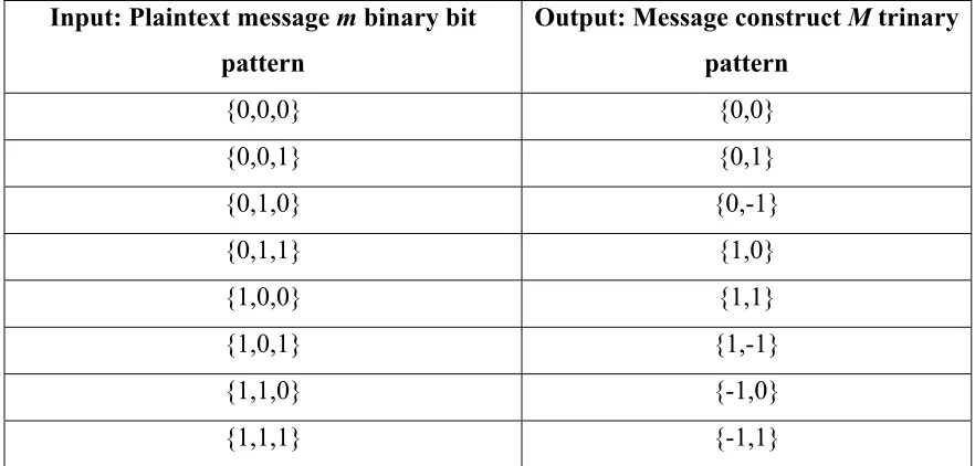
Input: Plaintext message m binary bit pattern

Output: Message construct M trinary pattern

{0,0,0} {0,0} {0,0,1} {0,1} {0,1,0} {0,-1} {0,1,1} {1,0} {1,0,0} {1,1} {1,0,1} {1,-1} {1,1,0} {-1,0} {1,1,1} {-1,1}

Table 4.6: Binary to trinary conversion

The transformation from binary to trinary increases the message density thereby allowing a larger binary plaintext message m to be stored in message construct M at a 3-to-2 ratio.

In order to provide plaintext awareness [2], a blinding polynomial r is generated with the same criteria as g per the following requirements:

- Polynomial r must contain drnumber of coefficients equal to ‘+1’, dr number of coefficients equal to ‘-1’ and the remaining N-2dr coefficients equal to ‘0’.

- To ensure security, generation of polynomial r needs to be random generated by means of a Random Number Generator (RNG) or Index Generation Function (IGF) detailed in [22].

Once a valid blinding polynomial r is selected, it is multiplied with the public key h. The final step is to add message m mod q to the product of r⊗hto produce the encrypted ciphertext message e.

) (mod q m

h r

Algorithm 4.6 was written to perform encryption which performs one polynomial star multiplication and a polynomial addition.

4.5

Decryption

Decryption reverses the encryption process to obtain the original message m. The first step in the decryption process is to obtain the intermediate polynomial a, from the ciphertext e, using the private polynomial keys fpand f [2].

) (modq e

f

a= ⊗ (19)

To ensure a high probability of decryption success, the coefficients of polynomial a must be adjusted so that all coefficients range from

2 q − to

2 q

instead of 0 to q. Details regarding why this step is required is discussed in the next section under Decryption Failures.

Once the coefficients are ‘balanced’, polynomial a is star multiplied by the inverse private key polynomial fp and reduced modulo p.

) (mod p a

f

b= _p ⊗ (20)

Input: r(x) – Blinding polynomial key r h(x) – Public key polynomial h

m(x) – Message polynomial to encrypt p - NTRUEncrypt ‘p’ parameter q – NTRUEncrypt ‘q’ parameter n – Degree size of polynomial

Output: e(x) – Ciphertext polynomial e=r⊗h+m(modq)

1: e(x)=r(x)⊗h(x)(modq)

2: e(x)=e(x)+m(modq)

Next, the original message construct M is derived by an additional module p reduction.

) (mod p b

M = (21)

A subtle step, that is not very well documented, is needed to correctly recover message construct M. Various coefficients throughout the algorithm are negative and therefore there exist instances where the multiplication of two negatives coefficients or modulo reduction of a negative coefficient results in a positive coefficient. Since the decrypted message construct M must maintain a trinary form, its coefficient need to be ‘balanced’ around zero the same way polynomial a was. Algorithm 4.7 was written to rotate a polynomial into a trinary form.

The final step in the decryption process is to convert the message construct M from a trinary form back to the original binary plaintext message m using Table 4.7.

Input: a(x) – Polynomial to convert p - NTRUEncrypt ‘p’ parameter n – Degree size of polynomial

Output: a(x) – Polynomial with trinary coefficients (-1, 0, 1)

Init: maxCoef = 2

1: for ( i = 0 to n ) 2: {

3: a(i) = Mod( a(i), p ) 4: if ( a(i) >= maxCoef ) 5: a(i) = a(i) – p

6: if ( a(i) <= ( -1 * maxCoef ) 7: a(i) = a(i) + p

8: }

Input: Message construct M trinary pattern

Output: Plaintext message m binary bit pattern {0,0} {0,0,0} {0,1} {0,0,1} {0,-1} {0,1,0} {1,0} {0,1,1} {1,1} {1,0,0} {1,-1} {1,0,1} {-1,0} {1,1,0} {-1,1} {1,1,1}

Table 4.7: Trinary to binary conversion

4.6

Decryption Failures

A decryption failure is when the plaintext message output of the decryption step does not match the original input message. NTRUEncrypt is unique to other PCKS in that, with standard parameters, ciphertext can fail to decrypt [48].

Given a polynomial of the form:

( )

1 2 2 1 1 0

0X a X a X a X q

a X a N N − − + + + =

The minimum and maximum coefficients are defined as: } ,..., , min{ )) (

(a X = a₀ a₁ a_N−1

Min , }Max(a(X))=max{a₀,a₁,...,a_N−1 The width of a polynomial is the polynomial’s range:

) ( ( )) ( ( )) (

(a X Max a X Min a X

Width = −

To understand decryption failures, Equation 19 utilizes the following substitutions:

) (modq e

f a= ⊗

Substitution for: e=r⊗h+m(mod q)

) (modq m f h r f

Substitution for: h= pf_q ⊗g(modq) ) (modq m f g pf r f

a= ⊗ ⊗ _q ⊗ + ⊗

Reduce: f ⊗ f_q ≡1(modq) ) (modq m f g p r

a= ⊗ ⊗ + ⊗

Since the coefficients of r, g, f and m are small, relative to q, their products will have a small Width [50]. The objective is to find a modulo q interval that results in a successful decryption, such that:

) (mod ) 1 ( ) 1 ( ) 1 ( ) 1 ( ) 1 ( ) 1

( r p g f m q

a = ⊗ ⊗ + ⊗

If an incorrect modulo q interval is chosen, a decryption failure will occur since the modulo q is incorrectly ‘zeroing’ out the coefficients of the polynomial. A successful decryption occurs when the degree-one-or-higher terms of the inverse polynomial fp cancel out, instead of the module q ‘zeroing’ out the terms.

A ‘gap’ decryption failure occurs when Width ≥ q, while a ‘wrap’ decryption failure occurs if Width < q. With either failure, the resulting message m will be incorrect by some multiple of q mod p [50]. The probability of a decryption failure can be

significantly reduced if the modulo q interval is adjusted such that the polynomial coefficients are centered on zero and range from

2 q − to

2 q

instead of 0 to q. Algorithm 4.8 was written to ‘balance’ a polynomial by forcing all coefficients outside into the range of

2 q − to

2 q

4.7

Why Decryption Works

For a cryptosystem to be useful, it must consistently be able to reproduce the original plaintext message, from ciphertext, without any errors. The steps involved in the encryption and decryption process constrain the various polynomials to modulo p or module q space. The encryption process combines several small modulo p constrained polynomials together to form a larger modulo q constrained polynomial [37]. Since the initial polynomials are constrained to a small modulo p, modulo reduction by q has no affect on the polynomial coefficients. However, the steps involved in decryption start with a polynomial constrained to the large modulo q space and work backwards reducing the polynomials to the smaller modulo p space.

Starting from the encrypted ciphertext e and working backwards, Figure 4.1 illustrates the necessary variable substitutions to obtain the original plaintext c.

Input: f(x) – Polynomial to balance n – Degree size of polynomial q – NTRUEncrypt ‘q’ parameter

Output: f(x) – Balance polynomial around 2 q

Init: maxCoef = 2 q

1: For (i = 0 to n) {

2: If( f(i) > maxCoef ) 3: f(i) = f(i) – q 4: If( f(i) < -maxCoef ) 5: f(i) = f(i) + q }

Figure 4.2: Flow chart from encrypted ciphertext e to plaintext c

Starting with the original ciphertext equation (18), substitutions for variables e and h using Equations (19) and (17) respectively results in an expanded definition of variable a [Substitution 1] in Figure 4.2. The multiplicative inverse identity of Equation (15) and the substitution of the plaintext definition of Equation (20) reduces the definition of variable a to three variables p, r and m [Substitution 2]. The modulo q reduction of this step does not affect any coefficients as long as the rules pertaining to q being large relative to p are enforced. The final [Substitution 3], performs a modulo reduction p which cancels out all terms except for the desired plaintext message m.

) (modq m h r

e = ⊗ +

Equation (19) Equation (17)

Equation (18)

) (mod

1 q

f

f_q ⊗ ≡

) (modq m f r pf

a = _q ⊗ ⊗ +

) (mod q e

f

a= ⊗ h= pf_q ⊗g(mod q)

Equation (15)

) (mod p a

f

c= _p⊗ _{Reduce (mod q)}

m r p

a = ⊗ +

Equation (20) m p r p f

c= _p ⊗ (mod )+

) (mod p m

c=

Reduce (mod p)

[Substitution 1]

[Substitution 2]

5 NTRUEncrypt Optimizations

The core mathematics involved in almost every step of the NTRU algorithm involves some form of polynomial multiplication. Techniques that reduce the execution time required for polynomial multiplication directly improves the efficiency of NTRU.

5.1

Star Multiplication

Recall standard star multiplication of two polynomials, a(x) and b(x), contained in ring R and both being N-degrees in size, is performed utilizing aforementioned Equation (14). The pseudo-code version used throughout the NTRUEncrypt algorithm is detailed in Algorithm 5.1.

Input: a(x) – First polynomial b(x) – Second polynomial

n – Size of polynomials a(x) and b(x) d – Size of output polynomial h(x)

m – Modulo value to apply to coefficients Output: c(x) = a(x)⊗b(x) in (Z/(c)Z)[x] / (xn _{– 1)}

Init: c(x) = 0, val = 0, exp = 0, i = 0, j = 0 1: For ( i = 0 to n )

{

2: If ( a(i) != 0 ) {

3: For ( j = 0 to n ) {

4: If ( b(j) != 0 ) { 5: exp = (i + j) (mod d) 6: val = c[exp] + a(i)b(i) 7: c[exp] = Mod(val, m) } }

} }

The convolution of two polynomials using traditional multiplication in code utilizes two nested loops as seen in Steps 1 and 3 of Algorithm 5.1. Step 5 calculates and stores the rotation amount, exp, of the exponents within ring R. Steps 6 and 7 perform the multiplication of the input polynomials, reduction modulo m, and adds the resulting product to the correct polynomial coefficient. One very simple optimization to Algorithm 5.1 is shown in Steps 2 and 4. These two ‘If’ checks prevent any further execution of the polynomial multiplication in Steps 5-7 if the coefficient of any polynomial equals zero. Though this optimization has no affect on non-zero coefficients, ‘Zero Check’ reduces the execution time required for generating the NTRUEncrypt private key polynomials since approximately 1/3 of the secret polynomial coefficients for f, g and r are chosen to equal zero per Section 4.3. Algorithm 5.1 requires very little RAM to execute, but has a growth rate of O(n2)

5.2

Karatsuba

The Karatsuba Algorithm (KA) was introduced in 1963 by Anatolii Alexeevitch Karatsuba [40] as a technique to improve the time required to multiply two polynomials. The technique reduces the number of coefficient multiplications involved in standard multiplication techniques, but at the expenses of utilizing extra additions [39].

5.3

Karatsuba Multiplication

In contrast to traditional multiplication, KA requires more RAM to execute, but decreases execution times by decomposing each input polynomial into several smaller polynomials.

Weimerskirch et al [39], demonstrates the steps required to multiply two, one degree, polynomials based on KA as follows given polynomials f(x) and g(x) in one pass:

x f f x

f( )= ₀ + ₁ , g(x)= g₀ +g₁x

Components of polynomials f(x) and g(x) are extracted and stored in three intermediate variables, fg0, fg1 and rfg as follows:

0 0

0 f g

The resulting product of h(x) = f(x)g(x) is performed as follows:

0 1

0 2

1( ) ( )

)

(x fg x r fg fg x fg

h = + _fg − − +

In comparison to traditional multiplication, which requires n2 = 22 = 4 multiplications and (n – 1)2 = (2 – 1)2 = 1 additions, the KA method requires 4 additions and 3

multiplications. KA therefore saves 1 multiplication, but required 3 additional additions [39].

5.4

Recursive Karatsuba (KM)

Polynomial multiplication using KA for only one iteration, as seen above, can be extended to incorporate recursion. The recursive KA method, referred to as KM in this thesis, is nothing more than ‘splitting’ the polynomials f(x) and g(x) into two halves and applying the aforementioned one-pass KA algorithm repeatedly until the polynomial size, n, is equal to 1.

Slight changes to the recursive version of KM presented by Weimerskirch et al [39] included constraining polynomials f(x) and g(x) to the ring, R, of truncated polynomials in steps 3b, 5, 12, and 13 or whenever multiplication of polynomials occurred. Also, a coefficient reduction modulo c is performed for any operation on a coefficient.

Given: f(x) = -1 – x, g(x) = -1 – x, n = 2, c = 3, threshold = 1 Find: h(x) = f(x)g(x) (mod c) in (Z/(c)Z)[x] / (xn – 1) using KM

Input: F(x) – First polynomial G(x) – Second polynomial

H(x) – Product of F(x) and G(x) in (Z/(c)Z)[x] / (xn – 1) n – Size of polynomials

c – Modulo value to apply to coefficients

cutOff – Minimum value of n for KM to execute Output: H(x) = F(x)⊗G(x) in (Z/(c)Z)[x] / xn – 1

Init: ls = n / 2, hs = n – ls, count = 0, 1: count = count + 1

2: If ( n = 1 ) {

If ( F(0) = 0 OR G(0) = 0 )

3a: Return 0;

Else

3b: Return H(x) = Mod( F(x)*G(x), c) in (Z/(c)Z)[x] / (xn – 1) }

4: If ( n < cutOff )

5: Star_Multiply(F(x), G(x), H(x), n, c) 6: FL = F0x0 … Flsxls

7: FH = Fls+1xls+1 … Fhsxhs 8: GL = G0x0 … Glsxls 9: GH = Gls+1xls+1 … Ghsxhs

10: FGL = FLGL = KM_STAR(FL, GL, FGL, ls, c) 11: FGH = FHGH = KM_STAR(FH, GH, FGH, ls, c) 12: Rfg = (FL + FH)(GL + GH)

= KM_STAR((FL + FH), (GL + GH), Rfg, hs, c) in (Z/(c)Z)[x] / (xn – 1)

13: H(x) = Mod((FGH(x2ls) + (Rfg – FGL – FGH)(xls) + FGL)) in (Z/(c)Z)[x] / (xn – 1)

Figure 5.1: KM Example

5.5

KM Performance

KM splits the input polynomial into two segments for each iteration of the algorithm. Figure 5.2 details the polynomial sizes (N) for each iteration for an initial N = 107. For Iteration 1 of KM, the original N = 107 is divided into two smaller polynomials of N = 53 and N = 54. Each iteration of the KM ‘splits’ the previous N in half, thereby forming a binary tree. As the binary tree grows, the number of polynomials increases while their respective N-size decreases until each branch of the tree is reduced to an N = 1 as shown in Step 2 of Algorithm 5.2. Depending on the initial N-size, the ‘splitting’ involved in KM quickly composes a large binary tree requiring significant memory.

Init: ls = n / 2 = 2 / 2 = 1, hs = n – ls = 2 – 1 = 1 6: FL= -1

7: FH= -1 8: GL = -1 9: GH = -1

10: F