Bidding Optimally in Concurrent Second-Price Auctions of
Perfectly Substitutable Goods
Enrico H. Gerding, Rajdeep K. Dash, David C. K. Yuen and Nicholas R. Jennings
University of Southampton, Southampton, SO17 1BJ, UK.{
eg,rkd,dy,nrj
}@ecs.soton.ac.uk
ABSTRACT
We derive optimal bidding strategies for a global bidding agent that participates in multiple, simultaneous second-price auctions with perfect substitutes. We first consider a model where all other bidders are local and participate in a single auction. For this case, we prove that, assuming free dis-posal, the global bidder should always place non-zero bids in all available auctions, irrespective of the local bidders’ valua-tion distribuvalua-tion. Furthermore, for non-decreasing valuavalua-tion distributions, we prove that the problem of finding the opti-mal bids reduces to two dimensions. These results hold both in the case where the number of local bidders is known and when this number is determined by a Poisson distribution. This analysis extends to online markets where, typically, auc-tions occur both concurrently and sequentially. In addition, by combining analytical and simulation results, we demon-strate that similar results hold in the case of several global bidders, provided that the market consists of both global and local bidders. Finally, we address the efficiency of the overall market, and show that information about the number of lo-cal bidders is an important determinant for the way in which a global bidder affects efficiency.
Categories and Subject Descriptors
I.2.11 [Distributed Artificial Intelligence]: Multiagent systems; J.4 [Social and Behavioral Sciences]: Economics
General Terms
Economics
Keywords
Vickrey Auctions, Simultaneous Auctions, Market Efficiency
1.
INTRODUCTION
The recent surge of interest in online auctions has resulted in an increasing number of auctions offering very similar or
Permission to make digital or hard copies of all or part of this work for personal or classroom use is granted without fee provided that copies are not made or distributed for profit or commercial advantage and that copies bear this notice and the full citation on the first page. To copy otherwise, to republish, to post on servers or to redistribute to lists, requires prior specific permission and/or a fee.
AAMAS ’07 Honolulu, Hawai’i
Copyright 2007 IFAAMAS .
even identical goods and services [9, 10]. In eBay alone, for example, there are often hundreds or sometimes even thou-sands of concurrent auctions running worldwide selling such substitutable items1. Against this background, it is essential
to develop bidding strategies that autonomous agents can use to operate effectively across a wide number of auctions. To this end, in this paper we devise and analyse optimal bid-ding strategies for an important yet barely studied setting — namely, an agent that participates in multiple, concur-rent (i.e., simultaneous) second-price auctions for goods that are perfect substitutes. As we will show, however, this anal-ysis is also relevant to a wider context where auctions are conducted sequentially, as well as concurrently.
To date, much of the existing literature on multiple auc-tions focuses either on sequential aucauc-tions [6] or on simulta-neous auctions for complementary goods, where the value of items together is greater than the sum of the individual items (see Section 2 for related research on simultaneous auctions). In contrast, here we consider bidding strategies for markets with multiple concurrent auctions and perfect substitutes. In particular, our focus is on Vickrey or second-price sealed bid auctions. We choose these because they require little communication and are well known for their capacity to in-duce truthful bidding, which makes them suitable for many multi-agent system settings. However, our results generalise to settings with English auctions since these are strategically equivalent to second-price auctions. Within this setting, we are able to characterise, for the first time, a bidder’s utility-maximising strategy for bidding simultaneously in any num-ber of such auctions and for any type of bidder valuation dis-tribution. In more detail, we first consider a market where a single bidder, called theglobal bidder, can bid in any number of auctions, whereas the other bidders, called thelocal bid-ders, are assumed to bid only in a single auction. For this case, we find the following results:
• Whereas in the case of a single second-price auction a bidder’s best strategy is to bid its true value, the best strategy for a global bidder is to bid below it.
• We are able to prove that, even if a global bidder re-quires only one item, the expected utility is maximised by participating in all the auctions that are selling the desired item.
• Finding the optimal bid for each auction can be an ar-duous task when considering all possible combinations. However, for most common bidder valuation
distribu-1To illustrate, at the time of writing, within eBay alone over
tions, we are able to significantly reduce this search space and thus the computation required.
• Empirically, we find that a bidder’s expected utility is maximised by bidding relatively high in one of the auctions, and equal or lower in all other auctions. We then go on to consider markets with more than one global bidder. Due to the complexity of the problem, we combine analytical results with a discrete simulation in order to nu-merically derive the optimal bidding strategy. By so doing, we find that, in a market with only global bidders, the dy-namics of the best response do not converge to a pure strat-egy. In fact it fluctuates between two states. If the market consists of both local and global bidders, however, the global bidders’ strategy quickly reaches a stable solution and we approximate a symmetric Nash equilibrium.
The remainder of the paper is structured as follows. Sec-tion 2 discusses related work. In SecSec-tion 3 we describe the bidders and the auctions in more detail. In Section 4 we in-vestigate the case with a single global bidder and characterise the optimal bidding behaviour for it. Section 5 considers the case with multiple global bidders and in Section 6 we address the market efficiency. Finally, Section 7 concludes.
2.
RELATED WORK
Research in the area of simultaneous auctions can be seg-mented along two broad lines. On the one hand, there is the game-theoretic and decision-theoretic analysis of simultane-ous auctions which concentrates on studying the equilibrium strategy of rational agents [3, 7, 8, 9, 12, 11]. Such analy-ses are typically used when the auction format employed in the concurrent auctions is the same (e.g. there are M Vick-rey auctions or M first-price auctions). On the other hand, heuristic strategies have been developed for more complex settings when the sellers offer different types of auctions or the buyers need to buy bundles of goods over distributed auc-tions [1, 13, 5]. This paper adopts the former approach in studying a market of M simultaneous Vickrey auctions since this approach yields provably optimal bidding strategies.
In this case, the seminal paper by Engelbrecht-Wiggans and Weber provides one of the starting points for the game-theoretic analysis of distributed markets where buyers have substitutable goods. Their work analyses a market consist-ing of couples havconsist-ing equal valuations that want to bid for a dresser. Thus, the couple’s bid space can at most contain two bids since the husband and wife can be at most at two geographically distributed auctions simultaneously. They de-rive a mixed strategy Nash equilibrium for the special case where the number of buyers is large. Our analysis differs from theirs in that we study concurrent auctions in which bidders have different valuations and the global bidder can bid in all the auctions concurrently (which is entirely possible given autonomous agents).
Following this, [7] then studied the case of simultaneous auctions with complementary goods. They analyse the case of both local and global bidders and characterise the bidding of the buyers and resultant market efficiency. The setting provided in [7] is further extended to the case of common values in [9]. However, neither of these works extend easily to the case of substitutable goods which we consider. This case is studied in [12], but the scenario considered is restricted to three sellers and two global bidders and with each bidder having the same value (and thereby knowing the value of
other bidders). The space of symmetric mixed equilibrium strategies is derived for this special case, but again our result is more general. Finally, [11] considers the case of concurrent
Englishauctions, in which he develops bidding algorithms for buyers with different risk attitudes. However, he forces the bids to be the same across auctions, which we show in this paper not always to be optimal.
3.
BIDDING IN MULTIPLE AUCTIONS
The model consists ofM sellers, each of whom acts as an auctioneer. Each seller auctions one item; these items are complete substitutes (i.e., they are equal in terms of value and a bidder obtains no additional benefit from winning more than one item). TheM auctions are executed concurrently; that is, they end simultaneously and no information about the outcome of any of the auctions becomes available until the bids are placed2. However, we briefly address markets with both sequential and concurrent auctions in Section 4.4. We also assume that all the auctions are equivalent (i.e., a bidder does not prefer one auction over another). Finally, we assume free disposal (i.e., a winner of multiple items incurs no additional costs by discarding unwanted ones) and risk neutral bidders.
3.1
The Auctions
The seller’s auction is implemented as a Vickrey auction, where the highest bidder wins but pays the second-highest price. This format has several advantages for an agent-based setting. Firstly, it is communication efficient. Secondly, for the single-auction case (i.e., where a bidder places a bid in at most one auction), the optimal strategy is to bid the true value and thus requires no computation (once the valuation of the item is known). This strategy is also weakly dominant (i.e., it is independent of the other bidders’ decisions), and therefore it requires no information about the preferences of other agents (such as the distribution of their valuations).
3.2
Global and Local Bidders
We distinguish between global and local bidders. The former can bid in any number of auctions, whereas the latter only bid in a single one. Local bidders are assumed to bid according to the weakly dominant strategy and bid their true valuation3.
We consider two ways of modelling local bidders: static and
dynamic. In the first model, the number of local bidders is assumed to be known and equal to N for each auction. In the latter model, on the other hand, the average number of bidders is equal toN, but the exact number is unknown and may vary for each auction. This uncertainty is modelled using a Poisson distribution (more details are provided in Section 4.1).
As we will later show, a global bidder who bids optimally has a higher expected utility compared to a local bidder, even though the items are complete substitutes and a bidder only requires one of them. However, we can identify a number of compelling reasons why not all bidders would choose to bid globally. Firstly, participation costs such as entry fees and time to set up an account may encourage occasional users to
2Although this paper focuses on sealed-bid auctions, where
this is the case, the conditions are similar for last-minute bidding in English auctions such as eBay [10].
3Note that, since bidding the true value is optimal for local
participate in auctions that they are already familiar with. Secondly, bidders may simply not be aware of other auctions selling the same type of item. Even if this is known, how-ever, additional information such as the distribution of the valuations of other bidders and the number of participating bidders is required for bidding optimally across multiple auc-tions. This lack of expert information often drives a novice to bid locally. Thirdly, an optimal global strategy is harder to compute than a local one. An agent with bounded ratio-nality may therefore not have the resources to compute such a strategy. Lastly, even though a global bidder profits on
average, such a bidder may incur a loss when inadvertently winning multiple auctions. This deters bidders who are ei-ther risk averse or have budget constraints from participating in multiple auction. As a result, in most market places we expect a combination of global and local bidders.
In view of the above considerations, human buyers are more likely to bid locally. The global strategy, however, can be effectively executed by autonomous agents since they can gather data from many auctions and perform the required calculations within the desired time frame.
4.
A SINGLE GLOBAL BIDDER
In this section, we provide a theoretical analysis of the opti-mal bidding strategy for a global bidder, given that all other bidders are local and simply bid their true valuation. Af-ter we describe the global bidder’s expected utility in Sec-tion 4.1, we show in SecSec-tion 4.2 that it is always optimal for a global bidder to participate in the maximum number of auctions available. In Section 4.3 we discuss how to signifi-cantly reduce the complexity of finding the optimal bids for the multi-auction problem, and we then apply these methods to find optimal strategies for specific examples. Finally, in Section 4.4 we extend our analysis to sequential auctions.
4.1
The Global Bidder’s Expected Utility
In what follows, the number of sellers (auctions) isM ≥2 and the number of localbidders is N ≥1. A bidder’s valuation
v ∈ [0, vmax] is randomly drawn from a cumulative distri-butionF with probability densityf, wheref is continuous, strictly positive and has support [0, vmax]. F is assumed to be equal and common knowledge for all bidders. A global bidBis a set containing a bidbi∈[0, vmax] for each auction 1≤i≤M (the bids may be different for different auctions). For ease of exposition, we introduce the cumulative distri-bution function for the first-order statisticsG(b) =F(b)N
∈
[0,1], denoting the probability of winning a specific auction conditional on placing bidb in this auction, and its proba-bility densityg(b) =dG(b)/db=N F(b)N−1f(b). Now, the
expected utilityU for a global bidder with global bidBand valuationvis given by:
U(B, v) =v
1− Y
bi∈B
(1−G(bi))
− X
bi∈B
Z bi 0
yg(y)dy (1)
Here, the left part of the equation is the valuation mul-tiplied by the probability that the global bidder wins at least one of the M auctions and thus corresponds to the expected benefit. In more detail, note that 1−G(bi) is the probability of not winning auction i when bidding bi, Q
bi∈B(1−G(bi)) is the probability of not winning any
auc-tion, and thus 1−Q
bi∈B(1−G(bi)) is the probability of
winning at least one auction. The right part of equation 1 corresponds to the total expected costs or payments. To see
the latter, note that the expected payment of a single second-price auction when biddingbequalsRb
0yg(y)dy(see [6]) and
is independent of the expected payments for other auctions. Clearly, equation 1 applies to the model withstaticlocal bid-ders, i.e., where the number of bidders is known and equal for each auction (see Section 3.2). However, we can use the same equation to modeldynamiclocal bidders in the follow-ing way:
Lemma 1 By replacing the first-order statisticG(y)with
ˆ
G(y) =eN(F(y)−1), (2)
and the corresponding density function g(y) with gˆ(y) =
dGˆ(y)/dy = N f(y)eN(F(y)−1), equation 1 becomes the ex-pected utility where the number of local bidders in each auc-tion is described by a Poisson distribuauc-tion with averageN
(i.e., where the probability that nlocal bidders participate is given byP(n) =Nne−N/n!).
Proof To prove this, we first show that G(·) andF(·) can
be modified such that the number of bidders per auction is given by a binomialdistribution (where a bidder’s decision to participate is given by a Bernoulli trial) as follows:
G0(y) =F0(y)N = (1−p+p F(y))N, (3)
where pis the probability that a bidder participates in the auction, andN is the total number of bidders. To see this, note that not participating is equivalent to bidding zero. As a result, F0(0) = 1−p since there is a 1−p probability
that a bidder bids zero at a specific auction, andF0(y) = F0(0) +p F(y) since there is a probability p that a bidder bids according to the original distributionF(y). Now, the average number of participating bidders is given byN=pN. By replacingpwithN/N, equation 3 becomesG0(y) = (1−
N/N + (N/N)F(y))N. Note that a Poisson distribution is given by the limit of a binomial distribution. By keeping
N constant and taking the limit N → ∞, we then obtain
G0(y) =eN(F(y)−1)= ˆG(y). This concludes our proof.
The results that follow apply to both the static and dynamic model unless stated otherwise.
4.2
Participation in Multiple Auctions
We now show that, for any valuation 0< v < vmax, a utility-maximising global bidder should always place non-zero bids in all available auctions. To prove this, we show that the ex-pected utility increases when placing an arbitrarily small bid compared to not participating in an auction. More formally,
Theorem 1 Consider a global bidder with valuation 0 <
v < vmax and global bid B, where bi ≤ v for all bi ∈ B.
Suppose B contains no bid for auction j ∈ {1,2, . . . , M}, then there exists abj>0such thatU(B ∪ {bj}, v)> U(B, v).
Proof Using equation 1, the marginal expected utility for
participating in an additional auction can be written as:
U(B ∪ {bj}, v)−U(B, v) =vG(bj)
Y
bi∈B
(1−G(bi))−
Z bj
0
yg(y)dy
Now, using integration by parts, we haveRbj
0 yg(y) =bjG(bj)−
Rbj
0 G(y)dyand the above equation can be rewritten as:
U(B ∪ {bj}, v)−U(B, v) =
G(bj)
v Y
bi∈B
(1−G(bi))−bj
+ Z bj
0
Let bj = , where is an arbitrarily small strictly positive value. Clearly,G(bj) andRbj
0 G(y)dyare then both strictly
positive (since f(y) > 0). Moreover, given that bi ≤ v <
vmax for bi∈ Band thatv >0, it follows thatvQb
i∈B(1−
G(bi))>0. Now, supposebj = 12vQb
i∈B(1−G(bi)), then
U(B ∪ {bj}, v)−U(B, v) = G(bj) h
1 2v
Q
bi∈B(1−G(bi))
i +
Rbj
0 G(y)dy > 0 and thus U(B ∪ {bj}, v) > U(B, v). This
completes our proof.
4.3
The Optimal Global Bid
A general solution to the optimal global bid requires the max-imisation of equation 1 inM dimensions, an arduous task, even when applying numerical methods. In this section, how-ever, we show how to reduce the entire bid space to two di-mensions in most cases (one continuous, and one discrete), thereby significantly simplifying the problem at hand. First, however, in order to find the optimal solutions to equation 1, we set the partial derivatives to zero:
∂U ∂bi
=g(bi)
v Y
bj∈B\{bi}
(1−G(bj)) −bi
= 0 (5)
Now, equality 5 holds either when g(bi) = 0 or when Q
bj∈B\{bi}(1−G(bj))v−bi = 0. In the dynamic model,
g(bi) is always greater than zero, and can therefore be ig-nored (sinceg(0) = N f(0)e−N and we assume f(y) > 0). In the static model, g(bi) = 0 only when bi = 0. How-ever, theorem 1 shows that the optimal bid is non-zero for
0< v < vmax. Therefore, we can ignore the first part, and
the second part yields:
bi=v Y
bj∈B\{bi}
(1−G(bj)) (6)
In other words, the optimal bid in auctioniis equal to the bidder’s valuation multiplied by the probability of not win-ning any of the other auctions. It is straightforward to show that the second partial derivative is negative, confirming that the solution is indeed a maximum when keeping all other bids constant. Thus, equation 6 provides a means to derive the optimal bid for auctioni, given the bids in all other auctions.
4.3.1
Reducing the Search Space
In what follows, we show that, for non-decreasing probabil-ity densprobabil-ity functions (such as the uniform and logarithmic distributions), the optimal global bid consists of at most two different values for any M ≥ 2. That is, the search space for finding the optimal bid can then be reduced to two con-tinuous values. Let these values be bhigh and blow, where
bhigh≥blow. More formally:
Theorem 2 Suppose the probability density function f is non-decreasing within the range[0, vmax], then the following proposition holds: givenv > 0, for any bi ∈ B, eitherbi =
bhigh,bi=blow, orbi=bhigh=blow.
Proof Using equation 6, we can produceM equations, one
for each auction, with M unknowns. Now, by combining these equations, we obtain the following relationship: b1(1−
G(b1)) =b2(1−G(b2)) =. . .=bm(1−G(bm)). By defining
H(b) =b(1−G(b)) we can rewrite the equation to:
H(b1) =H(b2) =. . .=H(bm) =v
Y
bj∈B
(1−G(bj)) (7)
In order to prove that there exist at most two different bids, it is sufficient to show that b = H−1(y) has at most two
solutions that satisfy 0≤b ≤vmax for anyy. To see this, suppose H−1(y) has two solutions but there exists a third bidbj6=blow 6=bhigh. From equation 7 it then follows that there exists aysuch thatH(bj) =H(blow) =H(bhigh) =y. Therefore,H−1(y) must have at least three solutions, which is a contradiction.
Now, note that, in order to prove thatH−1(y) has at most
two solutions, it is necessary and sufficient to show thatH(b) has at most one local maximum for 0≤b≤vmax. A suffi-cient conditions, however, is forH(b) to be strictly concave4.
The functionHis strictly concave if and only if the following condition holds:
H00(b) = d
db(1−b·g(b)−G(b)) =−
bdg db + 2g(b)
<0
(8) where H00(b) =d2H/db2. By performing standard
calcula-tions, we obtain the following condition for the static model:
b
(N−1)f(b)
F(b)+N
f0(b)
f(b)
>−2f or0≤b≤vmax, (9)
and similarly for the dynamic model we have:
b
N f(b) +f
0(b) f(b)
>−2f or0≤b≤vmax, (10)
where f0(b) = df /db. Since both f and F are positive, conditions 9 and 10 clearly hold for f0(b) ≥ 0. In other
words, conditions 9 and 10 show that H(b) is strictly con-cave when the probability density function is non-decreasing for 0≤b≤vmax, completing our proof.
Note from conditions 9 and 10 that the requirement of non-decreasing density functions is sufficient, but far from necessary. Moreover, condition 8 requiringH(b) to be strictly concave is also stronger than necessary to guarantee only two solutions. As a result, in practice we find that the reduction of the search space applies to most cases.
Given there are at most 2 possible bids,blowandbhigh, we can further reduce the search space by expressing one bid in terms of the other. Suppose the buyer places a bid ofblowin
Mlowauctions andbhighfor the remainingMhigh=M−Mlow auctions, equation 6 then becomes:
blow=v(1−G(blow))Mlow−1(1−G(bhigh))Mhigh,
and can be rearranged to give:
bhigh=G−1 1−
blow
v(1−G(blow))Mlow−1
1
Mhigh
! (11)
Here, the inverse function G−1(·) can usually be obtained quite easily. Furthermore, note that, ifMlow= 1 orMhigh= 1, equation 6 can be used directly to find the desired value.
Using the above, we are able to reduce the bid search space to a single continuous dimension, givenMloworMhigh. How-ever, we do not know the number of auctions in which to bid
blowandbhigh, and thus we need to searchM different com-binations to find the optimal global bid. Moreover, for each
4More precisely,H(b) can be either strictly convex or strictly
concave. However, it is easy to see thatH is not convex since
0 0.5 1 0
0.2 0.4 0.6 0.8 1
valuation (v)
b
id
fr
a
ct
io
n
(x
)
0 0.5 1
0 0.05 0.1
0.15 localM=2 M=4 M=6
valuation (v)
ex
p
ec
te
d
u
ti
li
[image:5.595.53.296.59.173.2]ty
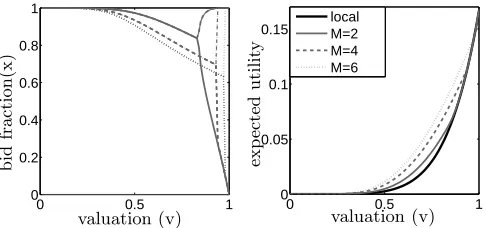
Figure 1: The optimal bid fractionsx=b/v and cor-responding expected utility for a single global bidder withN = 5static local bidders and varying number of auctions (M). In addition, for comparison, the dark solid line in the right figure depicts the expected util-ity when bidding locally in a randomly selected auc-tion, given there are no global bidders (note that, in case of local bidders only, the expected utility is not affected byM).
combination, the optimal blow and bhigh can vary. There-fore, in order to find the optimal bid for a bidder with valua-tionv, it is sufficient to search along one continuous variable
blow ∈ [0, v], and a discrete variable Mlow =M −Mhigh ∈
{1,2, . . . , M}.
4.3.2
Empirical Evaluation
In this section, we present results from an empirical study and characterise the optimal global bid for specific cases. Furthermore, we measure the actual utility improvement that can be obtained when using the global strategy. The results presented here are based on a uniform distribution of the val-uations withvmax= 1, and the static local bidder model, but they generalise to the dynamic model and other distributions (not shown due to space limitations). Figure 1 illustrates the optimal global bids and the corresponding expected util-ity for variousM and N = 5, but again the bid curves for different values of M and N follow a very similar pattern. Here, the bid is normalised by the valuationvto give the bid fractionx=b/v. Note that, when x= 1, a bidder bids its true value.
As shown in Figure 1, for bidders with a relatively low valuation, the optimal strategy is to submitM equal bids at, or very close to, the true value. The optimal bid fraction then gradually decreases for higher valuations. Interestingly, in most cases, placing equal bids is no longer the optimal strategy after the valuation reaches a certain point. A so-called pitchfork bifurcation is then observed and the optimal bids split into two values: a single high bid andM−1 low ones. This transition is smooth forM = 2, but exhibits an abrupt jump for M ≥ 3. In all experiments, however, we consistently observe that the optimal strategy is always to place a high bid in one auction, and an equal or lower bid in all others. In case of a bifurcation and when the valuation approachesvmax, the optimal high bid goes to the true value and the low bids go to zero.
As illustrated in Figure 1, the utility of a global bidder be-comes progressively higher with more auctions. In absolute terms, the improvement is especially high for bidders that have an above average valuation, but not too close tovmax. The bidders in this range thus benefit most from bidding
globally. This is because bidders with very low valuations have a very small chance of winning any auction, whereas bidders with a very high valuation have a high probability of winning a single auction and benefit less from participating in more auctions. In contrast, if we consider the utility rel-ative to bidding in a single auction, this is much higher for bidders with relatively low valuations (this effect cannot be seen clearly in Figure 1 due to the scale). In particular, we notice that a global bidder with a low valuation can improve its utility by up toM times the expected utility of bidding locally. Intuitively, this is because the chance of winning one of the auctions increases by up to a factorM, whereas the increase in the expected cost is negligible. For high valuation buyers, however, the benefit is not that obvious because the chances of winning are relatively high even in case of a single auction.
4.4
Sequential and Concurrent Auctions
In this section we extend our analysis of the optimal bidding strategy to sequential auctions. Specifically, the auction pro-cess consists ofRrounds, and in each round any number of auctions are running simultaneously. Such a combination of sequential and concurrent auctions is very common in prac-tice, especially online5. It turns out that the analysis for
the case of simultaneous auctions is quite general and can be easily extended to include sequential auctions. In the fol-lowing, the number of simultaneous auctions in round r is denoted byMr, and the set of bids in that round byBr. As before, the analysis assumes that all other bidders are local and bid in a single auction. Furthermore, we assume that the global bidders have complete knowledge about the number of rounds and the number of auctions in each round.
The expected utility in roundr, denoted byUr, is similar to before (equation 1 in Section 4.1) except that now additional benefit can be obtained from future auctions if the desired item is not won in one of the current set of simultaneous auctions. For convenience,Ur(Br,Mr) is abbreviated toUr in the following. The expected utility thus becomes:
Ur=v·Pr(Br)− X
bri∈Br
Z bri
0
yg(y)dy+Ur+1·(1−Pr(Br))
=Ur+1+ (v−Ur+1)Pr(Br)−
X
bri∈Br
Z bri
0
yg(y)dy, (12)
wherePr(Br) = 1−Q
bri∈Br(1−G(bri)) is the probability of
winning at least one auction in roundr. Now, we take the partial derivative of equation 12 in order to find the optimal bidbrj for auction jin roundr:
∂Us
∂brj
=g(brj)
(v−Us+1)
Y
bri∈Br\{brj}
(1−G(bri))−brj
(13)
5Rather than being purely sequential in nature, online
[image:5.595.317.554.595.643.2]Note that equation 13 is almost identical to equation 5 in Section 4.3, except that the valuationv is now replaced by
v−Ur+1. The optimal bidding strategy can thus be found by
backward induction (whereUR+1 = 0) using the procedure
outlined in Section 4.3.
5.
MULTIPLE GLOBAL BIDDERS
As argued in section 3.2, we expect a real-world market to exhibit a mix of global and local bidders. Whereas so far we assumed a single global bidder, in this section we consider a setting where multiple global bidders interact with one an-other and with local bidders as well. The analysis of this problem is complex, however, as the optimal bidding strat-egy of a global bidder depends on the stratstrat-egy of other global bidders. A typical analytical approach is to find the symmet-ric Nash equilibrium solution [9, 12], which occurs when all global bidders use the same strategy to produce their bids, and no (global) bidder has any incentive to unilaterally de-viate from the chosen strategy. Due to the complexity of the problem, however, here we combine a computational simula-tion approach with analytical results. The simulasimula-tion works by iteratively finding the best response to the optimal bid-ding strategies in the previous iteration. If this should result in a stable outcome (i.e., when the optimal bidding strate-gies remains unchanged for two subsequent iterations), the solution is by definition a (symmetric) Nash equilibrium.
5.1
The Global Bidder’s Expected Utility
In order to find a global bidder’s best response, we first need to calculate the expected utility given the global bidB and the strategies of both the other global bidders as well as the local bidders. In the following, letNg denote the number of
otherglobal bidders. Furthermore, let the strategies of the other global bidders be represented by the set of functions
βk(v),1≤k≤M, producing a bid for each auction given a bidder’s valuationv. Note that all other global bidders use the same set of functions since we consider symmetric equi-libria. However, we assume that the assignment of functions to auctions by each global bidder occurs in a random fashion without replacement (i.e., each function is assigned exactly once by each global bidder). Let Ω denote the set of all pos-sible assignments. Each such assignmentω∈Ω is a (M, Ng) matrix, where each entryωi,jidentifies the function used by global bidderjin auctioni. Note that the cardinality of Ω, denoted by|Ω|, is equal toM!Ng. Now, the expected utility
is the average expected utility over all possible assignments and is given by:
U(B, v) = 1
|Ω|
X
ω∈Ω
v
1− Y
bi∈B
(1−G˜ωi(bi))
− 1 |Ω|
X
ω∈Ω
X
bi∈B
Zbi 0
yg˜ωi(y)dy, (14)
where ˜Gωi(b) = G(b)·
QNg
j=1
Rb
0βωi,j(y)f(y)dy denotes the
probability of winning auctioni, given that each global bid-der 1 ≤ j ≤ Ng bids according to the function βωi,j, and
˜
gωi(y) = dG˜ωi(y)/dy. Here,G(b) is the probability of
win-ning an auction with only local bidders as described in Sec-tion 4.1, andf(y) is the probability density of the bidder valuations as before.
5.2
The Simulation
The simulation works by discretising the space of possible valuations and bids and then finding a best response to an
initial set of bidding functions. The best response is found by maximising equation 14 for each discrete valuation, which, in turn, results in a new set of bidding functions. These func-tions then affect the probabilities of winning in the next iter-ation for which the new best response strategy is calculated. This process is then repeated for a fixed number of iterations or until a stable solution has been found6.
Clearly, due to the large search space, finding the utility-maximising global bid quickly becomes infeasible as the num-ber of auctions and global bidders increases. Therefore, we reduce the search space by limiting the global bid to two dimensions where a global bidder bids high in one of the auctions and low in all the others7. This simplification is
justified by the results in Section 4.3.1 which show that, for a large number of commonly used distributions, the optimal global bid consist of at most two different values.
The results reported here are based on the following set-tings.8 In order to emphasize that the valuations are
dis-crete, we use integer values ranging from 1 to 1000. Each valuation occurs with equal probability, equivalent to a uni-form valuation distribution in the continuous case. A bid-der can select between 300 different equally-spaced bid lev-els. Thus, a bidder with valuation v can place bids b ∈ {0, v/300,2v/300, . . . , v}. The local bidders are static and bid their valuation as before. The initial set of functions can play an important role in the experiments. Therefore, to en-sure our results are robust, experiments are repeated with different random initial functions.
5.3
The Results
First, we describe the results with no local bidders. For this case, we find that the simulation does not converge to a stable state. That is, when there is at least one other global bidder, the best response strategy keeps fluctuating, irrespective of the number of iterations and of the initial state. The fluctua-tions, however, show a distinct pattern and alternate between two states. Figure 2 depicts these two states forNG= 10 and
M= 5. The two states vary most when there are at least as many auctions as there are global bidders. In that case, one of the best response states is to bid truthfully in one auction and zero in all others. The best response to that, however, is to bid an equal positive amount close to zero in all auc-tions; this strategy guarantees at least one object at a very low payment. The best response is then again to bid truth-fully in a single auction since this appropriates the object in that particular auction. As a result, there exists no stable solution. The same result is observed when the number of global bidders islessthan the number of auctions. This
oc-6This approach is similar to an alternating-move
best-response process with pure strategies [4], although here we consider symmetric strategies within a setting where an op-ponent’s best response depends on its valuation.
7Note that the number of possible allocations still increases
with the number of auctions and global bids. However, by merging all utility-equivalent permutations, we significantly increase computation speed, allowing experiments with rela-tively large numbers of auctions and bidders to be performed (e.g., a single iteration with 50 auctions and 10 global bidders takes roughly 30 seconds on a 3.00 Ghz PC).
8We also performed experiments with different precision,
0 200 400 600 800 1000 200
400 600 800 1000
valuation (v)
b
id
(b
)
[image:7.595.100.246.52.168.2]state 1 state 2
Figure 2: The two states of the best response strat-egy forM = 5 and Ng= 10 without local bidders.
5 10 15
0 1 2 3 4x 10
4
number of static local bidders
va
ri
a
n
ce
Ng= 5
Ng= 10
Ng= 15
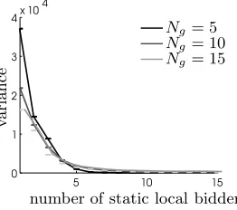
Figure 3: The variance of the best response strategy over 10 iterations and 10 experiments with different initial settings and M = 5. The errorbars show the (small) standard deviations.
curs since global bidders randomise over auctions, and thus they cannot coordinate and choose to bid high in different auctions.
As shown in Figure 2, a similar fluctuation is observed when the number of global bidders increases relative to the number of auctions. However, the bids in the equal-bid state (state 2 in Figure 2), as well as the low bids of the other state, increase. Moreover, if the number of global bidders is increased even further, a bifurcation occurs in the equal-bid state similar to the case without local bidders.
We now consider the best response strategies when both lo-cal and global bidders participate and each auction contains the same number of local bidders. To this end, Figure 3 shows the average variance of the best response strategies. This is measured as the variance of an actual best-response bid over different iterations, and then taking the average over the discrete bidder valuations. Here, the variance is a gauge for the amount of fluctuation and thus the instability of the strategy. As can be seen from this figure, local bidders have a large stabilising effect on the global bidder strategies. As a result, the best response strategy approximates a pure sym-metric Nash equilibrium. We note that the results converge after only a few iterations.
The results show that the principal conclusions in the case of a single global bidder carry over to the case of multiple global bidders. That is, the optimal strategy is to bid posi-tive in all auctions (as long as there are at least as many bid-ders as auctions). Furthermore, a similar bifurcation point is observed. These results are very robust to changes to the auction settings and the parameters of the simulation.
To conclude, even though a theoretical analysis proves dif-ficult in case of several global bidders, we can approximate a (symmetric) Nash equilibrium for specific settings using a
discrete simulation in case the system consists of both local and global bidders. Thus, our simulation can be used as a tool to predict the market equilibrium and to find the opti-mal bidding strategy for practical settings where we expect a combination of local and global bidders.
6.
MARKET EFFICIENCY
Efficiency is an important system-wide property since it char-acterises to what extent the market maximises social welfare (i.e. the sum of utilities of all agents in the market). To this end, in this section we study the efficiency of markets with either static or dynamic local bidders, and the impact that a global bidder has on the efficiency in these markets. Specifi-cally, efficiency in this context is maximised when the bidders with theM highest valuations in the entire market obtain a single item each. More formally, we define the efficiency of an allocation as:
Definition 1 Efficiency of Allocation. The efficiencyηK
of an allocationKis the obtained social welfare proportional to the maximum social welfare that can be achieved in the market and is given by:
ηK=
PNT
i=1vi(K)
PNT
i=1vi(K∗)
, (15)
where K∗ = arg maxK
∈KPNi=1T vi(K) is an efficient alloca-tion,Kis the set of all possible allocations, vi(K)is bidder
i’s utility for the allocationK∈ K, andNT is the total
num-ber of bidders participating across all auctions (including any global bidders).
Now, in order to measure the efficiency of the market and the impact of a global bidder, we run simulations for the markets with the different types of local bidders. The exper-iments are carried out as follows. Each bidder’s valuation is drawn from a uniform distribution with support [0,1]. The local bidders bid their true valuations, whereas the global bidder bids optimally in each auction as described in Sec-tion 4.3. The experiments are repeated 5000 times for each run to obtain an accurate mean value, and the final aver-age results and standard deviations are taken over 10 runs in order to get statistically significant results.
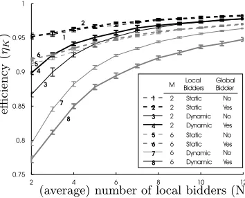
The results of these experiments are shown in Figure 4. Note that a degree of inefficiency is inherent to a multi-auction market with only local bidders [2].9 For example,
if there are two auctions selling one item each, and the two bidders with the highest valuations both bid locally in the same auction, then the bidder with the second-highest value does not obtain the good. Thus, the allocation of items to bidders is inefficient. As can be observed from Figure 4, how-ever, the efficiency increases when N becomes larger. This is because the differences between the bidders with the high-est valuations become smaller, thereby decreasing the loss of efficiency.
Furthermore, Figure 4 shows that the presence of a global bidder has a slightly positive effect on the efficiency in case the local bidders are static. In the case of dynamic bidders, however, the effect of a global bidder depends on the number of sellers. IfM is low (i.e., forM = 2), a global bidder sig-nificantly increases the efficiency, especially for low values of
9Trivial exceptions are when eitherM = 1 orN= 1 and
[image:7.595.113.244.207.323.2]2 4 6 8 10 12 0.75
0.8 0.85 0.9 0.95 1
1
3 4 5
6
7
8 2
M BiddersLocal GlobalBidder
2 Dynamic No 2 Dynamic Yes 2 Static No 2 Static Yes
6 Dynamic No 6 Dynamic Yes 6 Static No 6 Static Yes
2 1
3
4
5
6
7
8
(average) number of local bidders (N)
effi
ci
en
cy
(
ηK
[image:8.595.86.263.53.196.2])
Figure 4: Average efficiency for different market set-tings as shown in the legend. The error-bars indicate the standard deviation over the 10 runs.
N. ForM = 6, on the other hand, the presence of a global bidder has a negative effect on the efficiency (this effect be-comes even more pronounced for higher values ofM). This result is explained as follows. The introduction of a global bidder potentially leads to a decrease of efficiency since this bidder can unwittingly win more than one item. However, as the number of local bidders increase, this is less likely to happen. Rather, since the global bidder increases the num-ber of bidders, its presence makes an overall positive (albeit small) contribution in case of static bidders. In a market with dynamic bidders, however, the market efficiency depends on two other factors. On the one hand, the efficiency increases since items no longer remain unsold (this situation can oc-cur in the dynamic model when no bidder turns up at an auction). On the other hand, as a result of the uncertainty concerning the actual number of bidders, a global bidder is more likely to win multiple items (we confirmed this analyt-ically). As M increases, the first effect becomes negligible whereas the second one becomes more prominent, reducing the efficiency on average.
To conclude, the impact of a global bidder on the efficiency clearly depends on the information that is available. In case of static local bidders, the number of bidders is known and the global bidder can bid more accurately. In case of uncer-tainty, however, the global bidder is more likely to win more than one item, decreasing the overall efficiency.
7.
CONCLUSIONS
In this paper, we derive utility-maximising strategies for bid-ding in multiple, simultaneous second-price auctions. We first analyse the case where a single global bidder bids in all auctions, whereas all other bidders are local and bid in a single auction. For this setting, we find the counter-intuitive result that it is optimal to place non-zero bids in all auctions that sell the desired item, even when a bidder only requires a single item and derives no additional benefit from having more. Thus, a potential buyer can achieve considerable ben-efit by participating in multiple auctions and employing an optimal bidding strategy. For a number of common valua-tion distribuvalua-tions, we show analytically that the problem of finding optimal bids reduces to two dimensions. This consid-erably simplifies the original optimisation problem and can thus be used in practice to compute the optimal bids for any number of auctions.
Furthermore, we investigate a setting with multiple global
bidders by combining analytical solutions with a simulation approach. We find that a global bidder’s strategy does not stabilise when only global bidders are present in the market, but only converges when there are local bidders as well. We argue, however, that real-world markets are likely to contain both local and global bidders. The converged results are then very similar to the setting with a single global bidder, and we find that a bidder benefits by bidding optimally in multiple auctions. For the more complex setting with multiple global bidders, the simulation can thus be used to find these bids for specific cases.
Finally, we compare the efficiency of a market with multi-ple concurrent auctions with and without a global bidder. We show that, if the bidder can accurately predict the number of local bidders in each auction, the efficiency slightly increases. In contrast, if there is much uncertainty, the efficiency sig-nificantly diminishes as the number of auctions increases due to the increased probability that a global bidder wins more than two items. These results show that the way in which the efficiency, and thus social welfare, is affected by a global bidder depends on the information that is available to that global bidder.
In future work, we intend to extend the results to imperfect substitutes (i.e., when a global bidder gains from winning additional items), and to settings where the auctions are no longer identical. The latter arises, for example, when the number of (average) local bidders differs per auction or the auctions have different settings for parameters such as the reserve price.
8.
REFERENCES
[1] S. Airiau and S. Sen. Strategic bidding for multiple units in simultaneous and sequential auctions.Group Decision and
Negotiation, 12(5):397–413, 2003.
[2] P. Cramton, Y. Shoham, and R. Steinberg.Combinatorial
Auctions. MIT Press, 2006.
[3] R. Engelbrecht-Wiggans and R. Weber. An example of a multiobject auction game.Management Science, 25:1272–1277, 1979.
[4] D. Fudenberg and D. Levine.The Theory of Learning in
Games. MIT Press, 1999.
[5] A. Greenwald, R. Kirby, J. Reiter, and J. Boyan. Bid determination in simultaneous auctions: A case study. In
Proc. of the Third ACM Conference on Electronic
Commerce, pages 115–124, 2001.
[6] V. Krishna.Auction Theory. Academic Press, 2002. [7] V. Krishna and R. Rosenthal. Simultaneous auctions with
synergies.Games and Economic Behaviour, 17:1–31, 1996. [8] K. Lang and R. Rosenthal. The contractor’s game.RAND
J. Econ, 22:329–338, 1991.
[9] R. Rosenthal and R. Wang. Simultaneous auctions with synergies and common values.Games and Economic
Behaviour, 17:32–55, 1996.
[10] A. Roth and A. Ockenfels. Last-minute bidding and the rules for ending second-price auctions: Evidence from ebay and amazon auctions on the internet.The American
Economic Review, 92(4):1093–1103, 2002.
[11] O. Shehory. Optimal bidding in multiple concurrent auctions.Int. Journal of Cooperative Information Systems, 11:315–327, 2002.
[12] B. Szentes and R. Rosenthal. Three-object two-bidder simultaeous auctions:chopsticks and tetrahedra.Games and
Economic Behaviour, 44:114–133, 2003.
[13] D. Yuen, A. Byde, and N. R. Jennings. Heuristic bidding strategies for multiple heterogeneous auctions. InProc. 17th