Studies into the Detection of Buried Objects (Particularly Optical Fibres) in Saturated Sediment. Part 1: Background
T.G. Leighton and R.C.P. Evans ISVR Technical Report No 309
SCIENTIFIC PUBLICATIONS BY THE ISVR
Technical Reports are published to promote timely dissemination of research results by ISVR personnel. This medium permits more detailed presentation than is usually acceptable for scientific journals. Responsibility for both the content and any opinions expressed rests entirely with the author(s).
Technical Memoranda are produced to enable the early or preliminary release of information by ISVR personnel where such release is deemed to the appropriate. Information contained in these memoranda may be incomplete, or form part of a continuing programme; this should be borne in mind when using or quoting from these documents.
Contract Reports are produced to record the results of scientific work carried out for sponsors, under contract. The ISVR treats these reports as confidential to sponsors and does not make them available for general circulation. Individual sponsors may, however, authorize subsequent release of the material.
COPYRIGHT NOTICE
(c) ISVR University of Southampton All rights reserved.
Studies into the detection of buried objects (particularly optical fibres) in saturated sediment. Part 1: Background
T G Leighton and R C P Evans
2
UNIVERSITY OF SOUTHAMPTON
INSTITUTE OF SOUND AND VIBRATION RESEARCH FLUID DYNAMICS AND ACOUSTICS GROUP
Studies into the detection of buried objects (particularly optical fibres) in saturated sediment. Part 1: Background
by
T G Leighton and R C P Evans
ISVR Technical Report No. 309
April 2007
Authorized for issue by
Professor R J Astley, Group Chairman
ACKNOWLEDGEMENTS
TGL is grateful to the Engineering and Physical Sciences Research Council and Cable & Wireless for providing a studentship for RCPE to conduct this project.
iii
CONTENTS
ACKNOWLEDGEMENTS ii
CONTENTS iii
FIGURE CAPTIONS iv
ABSTRACT v
LIST OF SYMBOLS vi
1 INTRODUCTION 1
2 TELECOMMUNICATION CABLES 2
2.1 Armoured Cables 3
2.2 The Need for Repeaters 5
2.3 Cable Laying and Maintenance 6
3 DETECTION METHODS 9
3.1 Radar and Sonar Detection Systems 10
3.1.1 Electromagnetic Imaging 11
3.2 Nuclear Magnetic Resonance Imaging 16
3.3 Acousto-Optic Interaction 18
4 SUMMARY 20
FIGURE CAPTIONS
Figure 1 The structure of a typical lightweight fibre optic cable [6]. 4
Figure 2 The 4 m long ‘Sea Plow VI’ towed underwater vehicle can
bury cable to a depth of 1.1 m in the seabed at a maximum sea depth of
1 000 m. (From ROV Review 1993-94, WAVES magazine, Windate
Enterprises Inc., 5th Edition.)
7
Figure 3 The 3 m long ‘Seadog’ tracked underwater vehicle is used for
cable burial, tracking and repair at a maximum sea depth of 275 m.
(From ROV Review 1993-94, WAVES magazine, Windate Enterprises
Inc., 5th Edition.)
8
Figure 4 The characteristic attenuation length of electromagnetic
energy propagating through seawater [47].
v
ABSTRACT
Damaged submarine fibre optic telecommunication cables have, in the past, been located by the use of remotely operated underwater vehicles. These are fitted with sensors which have the capability to detect the metal shielding in the metallic cores used in cable technology. However, it is anticipated that the next generation of cables will have a much reduced metal content, their strength being derived from synthetic materials such as aramid fibres. Such structures will have greatly reduced contrast for detection by both electromagnetic and acoustic radiations transmitted from an underwater vehicle, to then propagate through the seabed and scatter off the cable. The detection of such cables will require new approaches.
This report is the first in a series of five written in support of the article “The detection by sonar of difficult targets (including centimetre-scale plastic objects and optical fibres) buried in saturated sediment” by T G Leighton and R C P Evans, written for a Special Issue of Applied Acoustics which contains articles on the topic of the detection of objects buried in marine sediment. Further support material can be found at http://www.isvr.soton.ac.uk/FDAG/uaua/target_in_sand.HTM.
LIST OF SYMBOLS
a An adjustment variable
A An empirically-derived constant relating to crack growth aEM Electromagnetic coil radius
ag Radius of curvature of a crack tip in a glass fibre
b An adjustment variable which appears in a number of separate equations B0 Magnetic field strength
C An empirically-derived constant relating to crack growth c0 Speed of light in a vacuum (3 × 10⁸ m s-1)
DA Diameter of cable armour wires
e Exponential constant (2.71828182) E Applied electric field
h Planck’s constant (6.626 × 10⁻³⁴ Js) h Rationalised Planck’s (h/2π)
I Spin
j Complex operator, −1
M0 Induced nuclear magnetisation me Electron mass (~9.109 × 10⁻³¹ kg)
vii P Polarisation
r0 Classical electron radius
Rg Gas constant (~8.314 kJ kg-1 mol-1 K-1)
t Time
TA Maximum load supported by cable armour Tabs Absolute temperature
V Volume (such that ∆V is the volume resolution of an image)
vp Phase velocity
x Cartesian co-ordinate in the horizontal plane
αdB Attenuation coefficient
χe Electric susceptibility of a dielectric
' e
ε Real effective permittivity ' '
e
ε Imaginary effective permittivity εEM Complex electromagnetic permittivity
' EM
ε Real component of complex electromagnetic permittivity ' '
EM
ε Imaginary component of complex electromagnetic permittivity ~
EM
ε Apparent permittivity εr Relative permittivity
εs Static permittivity
ε∞ Infinite frequency permittivity ε0 Permittivity of free space
η Avogadro’s number (6.023 × 1026 kg mol-1)
κ Boltzmann’s constant (1.380 × 10⁻²³ J K-1)
λ Wavelength
µ0 Electromagnetic permeability of free space
ν0 Larmor frequency
π Pi (≈ 3.141592654)
θL Effective loss tangent
ρ Resistivity of a sample volume
σB Back-scatter cross-section '
e
σ Real effective conductivity ' '
e
σ Imaginary effective conductivity σEM Complex electromagnetic conductivity
' EM
σ Real component of complex electromagnetic conductivity ' '
EM
σ Imaginary component of complex electromagnetic conductivity ~
EM
σ Apparent conductivity
σPa Applied stress
σR Rayleigh back-scattering cross-section
σ0 The DC conductivity
τPa Tensile strength
τr Relaxation time
ix
ω0 Natural circular frequency
ΨI Intrinsic signal-to-noise ratio
∇
Differential operator ∂
∂ ∂ ∂
∂ ∂
x, y, z
⎛ ⎝
⎜ ⎞
1 Introduction
This report is the first in a series which addresses the problem of the acoustic detection of objects, having dimensions of the order of centimetres, which are buried in underwater sediment. Specific example applications are considered, notably the detection of submarine optic fibre telecommunication cables. Particular attention is given to the poor acoustic impedance mismatch between the target and the sediment, and how it can be detected despite this.
The associated operational criteria (e.g., that the detection system should be deployed from a surface ship or from a remotely operated underwater vehicle) are not addressed in detail, being beyond the scope of this study. Rather, the study concentrates on the acoustic and signal processing aspects of the general problem. This, in turn, leads to a study of some fundamental processes related to the acoustic penetration of the seabed. As introduced above, objects of particular interest may be described as having properties which would make them difficult to detect. This condition implies that they are either small, compared to the wavelength of incident energy, or that they have similar physical properties to the surrounding medium. In either case, only a small proportion of incident acoustic energy will be scattered back towards the source. The detection problem is further complicated by the reverberant nature of the sediment medium.
The detection of submarine telecommunication cables is of particular interest to the sponsors of this research, Cable & Wireless. At present, such cables have a high acoustic contrast, being relatively large in size and having a high metallic content. In the near future, however, it is envisaged that cables could be made much smaller and almost entirely non-metallic. Conventional submarine cables, and cable maintenance systems, are introduced later in this report.
2
those judged most likely to succeed being developed further in subsequent reports (see section 4).
2 Telecommunication
Cables
Since the invention of the telegraph in the mid 19th century there has been an ever increasing need for high capacity communications links between cities, nations and continents. Early communications were restricted to low capacity lines made of copper wire carrying, at most, just tens of telephone conversations (or ‘channels’). In contrast, modern fibre optic links can convey tens of thousands of simultaneous transmissions of much better quality and security [1, 2].
The first oceanic telegraph cables were manufactured and laid in the 1850s. However, they had such limited capacity that they offered little improvement over the existing postal services. There was no significant improvement in the communications links between countries before the development of the radio in the early 1900s. It was not until 1956 that the first transoceanic telephone cable was laid, permitting 51 simultaneous conversations between New York and London [1].
Satellites first came into service in 1965 (Intelsat 1) and are now widely used for mobile communications and for where cables are not available. The quality they provide is improving all the time, although they still do not match the security and economy of undersea systems [1].
By the early 1980s the capacity of copper cables had increased to over 7 500 channels. In 1988 came the first fibre optic transatlantic system (TAT-8), with a capacity of 40 000 channels, stretching between the United States, Great Britain and France. Although much copper cable still exists, fibre optic cables have become the standard for high capacity, low cost transoceanic telecommunications.
October, 2000, when it will connect the US with France, Denmark, the UK, Germany and the Netherlands [3].
To keep the network growing and in good repair, ships and undersea vehicles are used for cable laying, burial and maintenance. These must be equipped with the most cost-effective technology on offer to meet the high levels of service required in the coming decades.
This project anticipates one of these technological challenges: It is envisaged that non-metallised fibre optic cables will become commercially available in the near future. Despite being lighter in weight and more flexible than metallised cables they have one major drawback; they are undetectable by present day cable maintenance systems. A new type of detection system is required to overcome this problem.
A brief overview of existing fibre optic systems and cable maintenance technology is presented in the following sections. The structure and composition of modern fibre optic cables is detailed in section 2.1. The present need for repeater systems is introduced in section 2.2. It is the possibility of unrepeatered long-haul cable systems and advances in cable technology that may lead to the use of non-metallised cables. Finally, the cable maintenance hardware, which could serve as a deployment platform for a buried cable detection system, is presented in section 2.3.
2.1 Armoured
Cables
4
Figure 1 The structure of a typical lightweight fibre optic cable [6].
If optic fibres are left exposed to seawater they become brittle and discoloured. This is caused by the process of hydrogen fixation whereby free hydroxyl ions diffuse from the water into the silica [4]. To prevent this from happening in telecommunication cables, the fibre unit is completely enclosed in a copper tube. Layers of metal wire and insulation are wrapped around this core element for strength and protection. The insulating layers are, typically, made of polyethylene and they help to maintain the cable structure. Cables that are buried or laid over rocky ground are sheathed in even more protective layers, the toughest being known as rock armour. These are built up in the same way and contain materials such as kevlar for added strength. A cross-section of a typical cable is shown in figure 1 [6].
TA =τPa×πDA ×n 2 4
(1)
where τPa is the tensile strength of steel (around 450 MPa), DA is the diameter of each wire and n is the total number of wires.
Typically, a load in excess of 10 tonnes can be applied before a cable will break. However, the resulting strain encourages microscopic cracks to grow in the fibres. According to Charles’ model [8], the rate of crack growth in an optic fibre in the direction, x, as a function of time, t, is given by
dx dt C x a A R T Pa N g N g abs = ⎛ ⎝ ⎜⎜ ⎞⎠⎟⎟ ⎛⎝⎜⎜ − ⎞⎠⎟⎟
σ 2 exp
(2)
where σPa is the applied stress, C, A and N are empirically derived constants, Rg is the gas constant, ag is the radius of curvature of the crack tip and Tabs is the absolute temperature.
The rate of crack growth (dx/dt) has been shown to be directly related to the operational lifetime of a cable [9]. Equation 2 indicates that the applied stress, σPa must be kept as small as possible in order to maximise this lifetime. This can be achieved by ensuring that the maximum allowable load on the armour, TA, is high. Hence, from equation 1, it can be seen that the operational lifetime of a cable is related to the diameter and number of armour wires. A cable such as that shown in figure 1 would be expected to have an operational lifetime in excess of 10 years in the seabed environment.
2.2 The Need for Repeaters
6
the original waveform exactly. Electrical power is supplied through the metal cable core.
‘Unrepeatered’ systems, which boost optical signals directly without the need to convert them into electrical signals, have also been developed. These are known as ‘erbium-doped fibre amplifiers’ (EDFAs) and are similar in principle to the laser [12, 13]. An ‘inverted population’ of photons is created in the doped region of a fibre by optical pumping [14]. Signals of the right wavelength can trigger ‘stimulated emission’ when they pass through this region of the fibre. This causes them to be amplified. With the development of remote EDFAs, systems of up to 2 000 km should be possible [15].
As cable technology continues to advance, unrepeatered transoceanic links are becoming a reality. The need for electrical conductors within the core will be removed and, with advanced materials providing strength and protection, metallised cables may become virtually redundant. It is anticipated that this new generation will be similar in diameter (~ 10 mm) to the smallest and lightest cables currently in use. As will be seen, however, non-metallised cables present a challenging detection problem.
2.3 Cable Laying and Maintenance
Cable systems are exposed to many ocean floor hazards: volcanoes; earthquakes; land slides; damage from the fishing industry; and even shark bites. Extensive sea-bottom surveys are conducted to enable engineers to lay cables in the safest areas. However, it has now become necessary to bury all the cables laid in continental shelf regions, where trawler fishing is prevalent [16].
Remotely operated vehicles (ROVs) are the primary apparatus used for cable burial and retrieval. They are designed to operate at sea depths of, typically, a few hundred metres (although ROVs that can operate at depths greater than 2 000 m are in existence [19]). There are two main types of cable maintenance ROV (described below), both of which are deployed and controlled from the surface vessel.
Figure 2 The 4 m long ‘Sea Plow VI’ towed underwater vehicle can bury cable to a
depth of 1.1 m in the seabed at a maximum sea depth of 1 000 m. (From ROV Review
1993-94, WAVES magazine, Windate Enterprises Inc., 5th Edition.)
The ‘plow’ is a simple machine, in principle at least, which is used for cable burial at a maximum speed of around 2 kilometres per hour (see figure 2). It is dragged over the seabed at a distance of 1 km or more behind the cable ship, and carves out a wedge shaped section 1 - 1.5 m deep in the sediment [20]. The cable is laid in this channel and the sediment replaced. The length of cable between the plow and the cable ship may be 2 km or more [21].
8
[image:20.595.110.523.117.402.2]an obstacle, such as a rock, can result in extensive damage. Hence, the route along which the cable is laid is planned very carefully in advance.
Figure 3 The 3 m long ‘Seadog’ tracked underwater vehicle is used for cable burial,
tracking and repair at a maximum sea depth of 275 m. (From ROV Review 1993-94,
WAVES magazine, Windate Enterprises Inc., 5th Edition.)
Once the cable has been laid, a different ROV is required if cable recovery or maintenance has to be performed. It is at this stage that a cable detection system is of vital importance.
The ‘seabed tractor’ is a robust cable maintenance vehicle which travels along the seabed on caterpillar tracks or skis at a maximum speed of 2 kilometres per hour (see figure 3). ROVs in this class are modular in design and have been manufactured in a range of sizes from less than 5 tonnes up to 100 tonnes. Similarly, their operational depth capabilities range from a few hundred metres up to 6 kilometres [22]. On-board camera and sonar equipment is used for navigation, and a magnetometer is used for the detection of metallised cables.
metal in a cable from a distance of a few metres. It is usual, however, to improve the visibility of a cable by the application of an alternating voltage (typically at 25 Hz) across its metal core. The resultant field stands out well against the background magnetic field of the Earth, enabling detection from a distance of 20 - 30 m. (The use of such technology will, of course, no longer be possible once non-metallised cables are brought into operation.)
Tools for the unearthing and cutting of cables are situated towards the front of the vehicle and high pressure water jets for burial are located at either the back or the front. Communication with the surface ship is achieved via an umbilical cable, which may carry data either optically or electronically, or via an acoustic link.
The modular design of the tractor allows a certain degree of flexibility in the mounting position of the forward-looking, navigational sonar. However, it is usually positioned at the front of the vehicle and as high up as possible to give the best field-of-view and to minimise the risk of damage. The possibility of adapting it for use in an imaging system was raised by the author in discussion with Cable & Wireless technicians. It was agreed that its position on the ROV and its present application restricted its direct use although a similar transducer, positioned towards the centre of the vehicle, might be more suitable.
3 Detection
Methods
Detection problems are often split into two steps [23]: The first involves the detection of potential targets without any attempt being made to classify them. The next step involves re-examining potential targets at a higher resolution to distinguish objects of interest from background clutter. Of course, it is often known whether or not a region is likely to contain objects of interest. The challenge lies in being able to reliably locate and classify them.
10
However, this approach is often unworkable (e.g., the object may be designed for covert use). In the particular application of buried telecommunication cables, such methods were quickly ruled out by Cable & Wireless as being too costly.
An alternative to the direct detection of an object would be to search for the collateral effects of its burial, i.e., ground disturbance due to cable laying. Acoustic, sub-bottom profiling systems suited to this task are currently available and are used in ocean bottom surveys [25, 26]. The drawback to this approach comes from the instability of the seafloor environment. For example, cable damage can be caused by undersea earthquakes that can also trigger slides in continental shelf regions, and mud-slides can completely hide any evidence of cable burial.
3.1 Radar and Sonar Detection Systems
The electromagnetic (EM) wave in radar is analogous, to a certain extent, to the pressure wave in sonar. The coupling between an EM wave and an electrically conductive medium causes absorption and scattering of a radar signal. This is similar to the interaction between a pressure wave and an acoustic medium which causes absorption and scattering of a sonar signal. Both radar and sonar systems rely on signal processing to separate useful information from background noise and clutter. In fact, as far as the signal processor is concerned, there is little to distinguish them [27]. There are, however, significant differences associated with the operating frequency ranges of the two systems. As a first approximation, a large back-scattered power may be achieved if the wavelength of incident radiation is less than the geometrical size of the target. Thus, for a 10 mm diameter cable in a water-saturated environment, this corresponds to frequencies higher than 6 GHz for radar and 50 kHz for sonar. At these frequencies, the attenuation coefficient of acoustic waves in water-saturated sand will be less than 30 dB m-1 [28]. In contrast, the absorption coefficient of EM waves will be greater than 300 dB m-1 (which is the absorption coefficient measured at 1 GHz in seawater [29]).
target by careful selection of the frequency spectrum of the incident radiation [30]. In the extreme case of highly non-linear scatterers, such as gas bubbles, resonant scattering can give up to 1000 times more back-scattered energy than simple geometric scattering [31].
For a complicated structure, such as a multi-layered telecommunication cable, the resonance spectrum cannot be determined easily. However, the feasibility of a resonance-based detection system can be investigated using homogeneous cylindrical targets, for which the spectrum can be determined [32].
In general, spatial resolution improves with increasing frequency. Unfortunately, the attenuation of sound in both seawater and sediments also increases with frequency [33]. Therefore, the operating frequency of an imaging system should be made as low as possible to ensure maximum penetration, but not so low that the target cannot be resolved. For certain target geometries, however, the back-scattered power at the receiver can actually increase at lower frequencies (see section 3.2 of the fourth report in this series).
It is clear from the numerous acoustic imaging systems in commercial use [34] that acoustic techniques are the preferred choice in underwater applications. Consider, for example, the ‘enhanced-bottom sonar system’ (EBSS) [35, 36, 37]; a device that was designed, specifically, to find cables suspended in the mid-ocean or buried in seabeds. It is based on the principle of matched filtering, whereby a high incident power and contrast may be achieved using a modulated pulse waveform [38]. Unfortunately, little has been published regarding this system.
Given that the attenuation coefficient of EM waves is considerably larger than that of acoustic waves (as noted above), it is reasonable to expect an acoustic system to perform better than an EM system in a water-saturated environment. This is particularly so in terms of achieving the maximum signal-to-noise ratio. Acoustic techniques will be investigated in greater detail in later reports in this series. Electromagnetic techniques are reviewed in the remainder of this section.
3.1.1 Electromagnetic Imaging
12
secondary source of EM radiation. For bound electrons, the ratio of the radiated power to the power per unit area in the incident beam, i.e., the back-scatter cross-section [39], is given by
(
)
[
]
σ π ω
ω ω ω γ
B r = − + 8 3 0 2 4 0
2 2 2 2 2
(3)
where ω is the frequency of the incident radiation, ω0 is the natural frequency, γ is the damping constant of the oscillating electrons and r0 is the classical electron radius. At low frequencies (ω<<ω0), this reduces to the Rayleigh scattering law1:
σ π ω
ω R r = ⎛ ⎝ ⎜ ⎞ ⎠ ⎟ 8 3 0 2 0 4 (4)
since γ <<ω0 [39]. Of course, a high back-scattered power can still be achieved over a wide frequency range since, as in the acoustic case, target features will diffract the incident radiation and will exhibit resonances resulting from their geometry. However, in order to assess the viability of EM imaging techniques in this investigation, it is first necessary to quantify absorption in the propagation medium. In sediments, the absorption of EM radiation is due to both conduction and dielectric effects [41]. When measurements are made at a single frequency, the complex permittivity, εEM = ′ − ′′εEM jεEM, and complex conductivity, σEM = ′ −σEM jσEM′′ , cannot be separated into two components of loss. However, in Maxwell’s equations [42] describing wave propagation, εEM and σEM always occur in the combination,
σEM+ jωεEM.
It is useful to define the following quantities:
1 The scattering of plane waves by objects that are small in comparison to the wavelength of the radiation is
Real effective permittivity, Real effective conductivity, Imaginary effective permittivity, Imaginary effective conductivity,
e e e ′ = ′ − ′′ ′ = ′ + ′′ ′′ = ′′ + ′ ′′ = ′′ − ′
ε ε σ
ω
σ σ ωε
ε ε σ
ω
σ σ ωε
EM EM
EM EM
EM EM
e EM EM
(5)
When measurements are made on a conducting dielectric, the apparent permittivity, ~
εEM = ′ − ′′εe jεe , and apparent conductivity, ~σEM = ′ − ′′σe jσe , are measured. The effective loss tangent, tanθL, is given by
tanθ σ σ ε ε L e e e e = − ′ ′′= ′′ ′ (6)
A range of equivalencies can be deduced. In particular, σEM+jωεEM =σ~EM = jωε~ EM
shows that the behaviour of a material can be specified by either its apparent permittivity or by its apparent conductivity.
If permeability is taken to be µ0 (the permeability of free space), the relationships between the apparent permittivity, ~εEM, phase velocity, vp, and attenuation, αdB, are given by [29]
(
)
v c
e c
p e L
dB e L
= ⎡ ′ + + ⎣ ⎢ ⎤ ⎦ ⎥ = × ⎡ ′ + − ⎣ ⎢ ⎤ ⎦ ⎥ − 0 0 2 1 2 10 0 0 2 1 2
2 1 1
20
2 1 1
ε
ε θ
α ω ε
ε θ
tan
log tan
(7)
(The factor, 20log e , is the scaling required to convert from nepers per metre to 10 decibels per metre.)
The principal loss mechanism in earth materials is the absorption of EM energy by water in the pore spaces. When an electrostatic field is applied to water, a polar liquid, a state of polarisation2 is induced. However, Brownian motion acts to prevent the free
2 In electrostatics, an applied field E produces polarisation charges in dielectric media and a polarisation P
related to the electric field by
14
rotation of the molecular dipoles [43]. Removal of the electrostatic field results in the polarisation decaying with a relaxation time, τr, which is characteristic of the Brownian motion at a particular temperature. The dielectric relaxation of pure water is described by the Debye equations with a single relaxation time:
′ = + −
+
∞ ∞
ε ε ε ε
ω τ
e s
r
1 2 2 and
(
)
′′ = −
+
∞
ε ε ε ωτ
ω τ e
s r
r 1 2 2
(8)
where εs is the ‘static permittivity’ and ε∞ is the ‘infinite frequency permittivity’ [44].
The presence of free ions in seawater increases conductivity and hence attenuation, although the frequency for peak attenuation (around 9 GHz at 0°C) is not significantly changed. An expression for the complex permittivity as a function of angular frequency in an electrolyte is given by
( )
( )( )
( )ε ω ε ε ε
ωτ
EM sa
r b j = + − + ∞ − ∞ −
1 1 1
(9)
which reduces to the Debye relation when the fitting parameters a b= =0 [45]. On the basis of equation (9), the complex permittivity can be found for a given temperature, frequency and ionic species. Combining this with a measurement of DC conductivity, σ0 (equivalent to σ′EMsince σ′′ =EM 0 ), and equations (5) to (7), the velocity of propagation and the attenuation constant can be found.
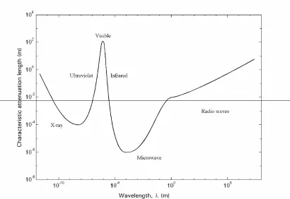
A graph illustrating the characteristic attenuation length of electromagnetic energy in seawater is presented in figure 4. This is the distance at which the amplitude of a propagating wave is reduced to 1 e of its initial value [41, 46]. The region of greatest transparency is around the optical wavelengths but these cannot penetrate the opaque seabed and are strongly scattered by suspended particles.
where χe is the electric susceptibility of the dielectric and εr is the relative permittivity. The permittivity of
Figure 4 The characteristic attenuation length of electromagnetic energy propagating
through seawater [47].
At high frequencies (for wavelengths λ < 10-8 m), where the frequency of the incident radiation will be close to the natural frequency of oscillating electric dipoles, the radiation scattered from a buried target will reach a peak. The classical limit for scattering from free electrons, known as Thomson scattering [48], is hω << m ce 02 (where h=h 2π and h is Planck’s constant). Quantum theory must be used for incident radiation having a wavelength that is less than this limit (λ < 2.424 × 10 -12 m).
It is within this wavelength range that Compton scattering3 occurs. Compton back-scatter imaging has successfully been used to detect land mines buried to depths of up to 7.5 cm in dry soil [49]. However, a practical source of X-rays of sufficiently high
3 It was shown by Compton that there is an increase in the wavelength of high energy photons (X-ray or
16
power to penetrate through up to 1.5 m of water-saturated sediment does not exist at the present time [50].
3.2 Nuclear Magnetic Resonance Imaging
The magnetic moment of an atom is the vector sum of the magnetic moments of the orbital motions and the spins of all the electrons in the atom. In 1897 the Irish physicist, Larmor, showed that the application of an aligning force (torque) to a spinning object causes a circular motion, known as ‘precession’. When subjected to an external magnetic field, the magnetic moment of an atom precesses at a frequency known as the ‘Larmor frequency’. This is directly proportional to the strength of the applied field [51].
Any material under the influence of a magnetic field may exhibit the distinctive Larmor resonance resulting from the precession of circulating electric currents (these being due to nuclear or electronic spin, or electron orbits). For a large number of nuclei, the net induced nuclear magnetisation is proportional to the magnetic field strength.
A strong magnetic field may be produced in a volume of material (such as the seabed) by passing an electric current through a coil of wire surrounding it. After a short time (~ second) a small bulk nuclear magnetisation will have developed, aligned in the same direction as the magnetic field. If the field is removed abruptly, by reducing the current in the coil to zero, the only remaining field is that of the Earth. Each of the nuclei experiences a small torque which attempts to realign it in the direction of the Earth’s magnetic field, but the property of spin possessed by the magnetisation ensures that it precesses at around 2.1 kHz [52]. This may be detected because of the effect it has on the dormant coil. Essentially, the coil is next to a freely rotating magnet and so, as demonstrated by Faraday, a small electromotive force will be induced in the coil [53].
on the requirements of the size of the device and the stability and homogeneity of the magnetic field in the target volume [54].
• Permanent magnets. These can generate fields of up to 0.3 tesler over volumes of many litres. Of primary concern are their temperature stability and weight, which can be up to 10 tonnes. To ensure field stability, temperature control better than 1 millidegree is required.
• Resistive Magnets. A medical, whole-body imaging NMRI scanner, generating a modest internal field of 0.15 tesler, can consume up to 60 kW of electrical power. Hence, there is a design compromise between weight and power consumption, though most designs weigh less than 10 tonnes.
• Superconducting Magnets. These represent the majority of magnets manufactured for medical NMRI systems. They possess the advantages of very high fields (up to 10 tesler) and excellent stability. However, the establishment of the magnetic field requires a large amount of energy (~ megajoules).
The volume resolution of the image, ∆V, for a range of nuclei in a uniform magnetic field, B0, can be approximated from the following expression [55]:
B V M
T a n
I abs EM
r 0
0
5 12
16 15
∆ = Ψ ⎛
⎝ ⎜ ⎞ ⎠ ⎟ πκ ρ τ (10)
where ΨI is the intrinsic signal-to-noise ratio, M0 is the induced nuclear magnetisation, κ is Boltzmann’s constant, Tabs is the absolute temperature in the sample volume, aEM is the coil radius, ρ is the resistivity of the sample volume, n is the number of sample measurements and τr is the relaxation time.
The induced nuclear magnetisation for one kilomole of substance in a volume of 1 m3 and in a field of 1 tesler is given by
(
)
M h I I
Tabs 0 0 2 2 1000 1 3
= ην +
κ
(11)
18
Consider the magnetisation of the hydrogen nuclei of water at 4 °C in a field of 1 tesler. The specific gravity of water is taken to be unity and the molecular weight to be 18. Thus, one litre of water weighs 1 kg and contains 1 000 / 18 moles. Using the above equation (where ν0 = 42.5749 MHz and I = 1/2), the magnetisation of a 1 mol l-1 solution is 3.1348 × 10⁻⁵ A m-1. Therefore, the magnetisation of water is
M0 = 3.1348 × 10-5× 2 × 1 000 / 18 = 1.742 × 10⁻³ A m-1.
The extra factor of 2 is introduced because there are two atoms of hydrogen per water molecule.
The expression in equation (10) applies to a uniform magnetic field such as that produced inside a medical scanner. In order to obtain sub-bottom images of the seabed, an alternative arrangement is required. A solution would be to use a magnetic coil positioned close to the surface of the seabed such that the imaging volume would still be within the ‘fringe field’ of the magnet (i.e., the field outside of the coil). The drawback to this approach is that the fringe field is, generally, much weaker and less uniform than the field at the centre of the coil.
A reasonable estimate of the field strength necessary to achieve a volume resolution of 1 ml using a surface coil can be obtained using equation (10). If the radius of the coil, aEM, is 1.5 m and given ΨI = 30:1, ρ = 1 Ω m, n = 256 and τr = 25 ms, a magnetic field strength of around 1.4 tesler is required. Only a superconducting magnet would be capable of generating such a high field strength (as noted above). The cost of deploying such a magnet, weighing several tonnes, from an underwater platform makes this technique unfeasible.
3.3 Acousto-Optic
Interaction
• The Faraday Effect. The propagation of light through a material can be influenced by an external magnetic field. In particular, the plane of vibration of linearly polarised4 light incident on a piece of glass is rotated when a strong magnetic field is applied in the direction of propagation. This relationship between electromagnetism and light was discovered by Faraday in 1845 and is also known as the magneto-optic effect [56].
• The Kerr and Pockels Effects. An isotropic transparent substance becomes birefringent when placed in an electric field. In other words, the material displays two different indices of refraction, one parallel and one perpendicular to the applied field. This effect was discovered by Kerr in 1875 [56]. Another important electro-optical effect was studied by Pockels in 1893. In certain crystals that lack a centre of symmetry, the induced birefringence is proportional to the first power of the applied electric field. Of the 32 classes of crystal symmetry, the 20 piezo-electric classes may exhibit the Pockels effect [56].
• Photo-Elasticity. Normally transparent isotropic substances can be made optically anisotropic by the application of mechanical stress. This is the oldest known non-linear optical interaction, also known as the ‘elasto-optic effect’, having been discovered by Brewster in 1816 [58]. Pockels gave a phenomenological formulation of the effect in 1890 that was regarded as adequate until recently5. In 1914, Brillouin predicted that light could be scattered by thermal fluctuations. This was related to the photo-elastic effect by considering the fluctuations as thermally-excited acoustic waves. The diffraction of light from coherently generated acoustic waves (‘acousto-optic diffraction’) was later observed [59].
• Micro-Bending Losses. The EM field of a guided wave in an optic fibre penetrates into the fibre cladding. At a bend, the field at the outside has to travel
4 Light is described as being ‘linearly’ (or plane) polarised if its electric field resides entirely in one plane, the
‘plane of vibration’. If the electric field vector rotates with constant angular frequency and constant magnitude in the direction of propagation, then the radiation is described as being ‘circularly’ polarised. If its magnitude changes, the radiation is ‘elliptically’ polarised [57].
5 The Pockels formulation has been shown to be inadequate when applied to shear deformations in birefringent
20
faster than that at the inside to maintain the phase relationship in the mode. At some distance from the fibre the speed of the wave will reach the speed of light in the surrounding medium, requiring energy at larger radii to be radiated. The proportion of optical power in the bend region that is dissipated in this way increases rapidly as the bend radius decreases [4].
Systems based on the magneto- and electro-optic effects are impractical for the detection of buried fibre optic cables. The attenuation of EM waves in seawater is very large over most of the frequency spectrum (300 dB m-1 at 1 GHz [29]) and a magnet capable of producing a significant magnetisation at a range of 1.5 m in water-saturated sand would be too costly to deploy.
Systems based on the photo-elastic effect and micro-bending losses seem far more promising. If an acoustic source mounted on an ROV were to be focused upon the cable, the stresses generated within the fibre could cause an observable change in the optical back-scatter profile. Alternatively, a directional, ship-mounted acoustic source of sufficiently high power (such as one designed to remotely detonate underwater mines [60]) might be used to first locate, or even map, the cables.
It is estimated that an acoustic pressure amplitude at the cable in excess of 100 kPa at a frequency of around 100 kHz would be required to achieve an observable effect [61]. The details of the acousto-optic phenomena that could be exploited, and the practicalities of their use in a real system, will be presented in a later report [61].
4 Summary
Non-invasive acoustic and electromagnetic techniques have been compared. The evidence suggests that acoustic systems are likely to be of greater use in the underwater environment.
Subsequent reports [61-64] detail various facets of the study to investigate the detection of targets buried in saturated sediment, primarily through acoustical or acoustics-related methods. Although steel targets are included for comparison, the major interest is in targets (polyethylene cylinders and optical fibres) which have a poor acoustic impedance mismatch with the host sediment. The reports will discuss the features which would be important considerations in the design of a detection system. They include a description of the construction and testing of an experimental rig and the associated signal processing system [62]. The laboratory apparatus includes a physical model of an area of the seafloor that is typical of the environment in which cables are buried. The nature of the acoustic transmission media are considered carefully, with a view to designing an effective transducer system [62]. The design of the laboratory test system will be described in the second report of this series [62]. It comprised a large, filled steel tank, part-filled with water-saturated sand. The average depth of the sediment was 50 cm, and the total depth of water and sediment within the tank was 116 cm. A pair of focused, acoustic transducers were designed and fabricated from a pressure-release material. These were mounted above the sediment and positioned using an automated, computer-controlled system [62].
22
The relatively high attenuation associated with the sediment had obvious implications for the transducer system. It was necessary for the source to develop a high sound pressure level in order for acoustic energy to penetrate into the sediment. The required amplitude is dependent on the reverberation level within the medium (since volume reverberation acts to mask acoustic signals back-scattered by the target), and the scattering strength of the target. The background noise level and the dynamic range of the receiver system were also important. If the background noise is relatively low, the required source level is dependent on the sensitivity of the receiver.
Geometrically-focused acoustic reflectors were used in the laboratory. This provided a cost-effective way of achieving a relatively high acoustic power and a narrow beamwidth, with a single hydrophone acting as either a source or receiver. (It should be noted that this solution was specifically intended for laboratory use. If the techniques described in this report were to be used in the field, a ruggedised transducer system would be required.) The performance of the transducers was modelled using ray tracing theory. It was noted that this theory does not take account of rim and surface diffraction effects. These were kept to a minimum by specifying a close surface tolerance of less than 1/20 of a wavelength. The free-field performance of the transducers was found to be in good agreement with that predicted by the model [62].
Those properties of the seawater-seabed interface which could seriously degrade the performance of a detection system will also be discussed in the third report in this series [63]. The fourth report will discuss the signal processing requirements of the detection system [64]. Both waveform-dependent and target-dependent processing techniques are considered. The latter of these requires knowledge of the scattering properties of the object being sought. Hence, the theory of resonant scattering from cylinders and spheres will be reviewed. By calculating the back-scattering cross-sections of the targets, it will be shown how it is possible to select an optimal frequency range for the detection system. The report will show how these results can be incorporated directly into the detection algorithms in an attempt to make them target specific [64].
experiments proved to be very successful in detecting objects buried between 25 and 30 cm deep in the sediment.
Matched filtering was shown to be useful in an environment dominated by noise or clutter. This was an important finding in light of the investigation undertaken in the third [63] report of the series, where it was noted that surface roughness can give rise to an increase in both background noise and clutter at the receiver [64].
The fourth report will show how target optimisation techniques resulted in a small increase in the average signal-to-noise ratio at the output of the system, and better localisation of the targets within the sediment. However, in terms of overall performance, this approach did not perform significantly better than waveform dependent optimal filtering [64].
The fourth report will report on how synthetic aperture techniques were also investigated in an attempt to achieve the best possible performance from the system. In that study the synthesised aperture approach has the potential for achieving a high signal-to-noise ratio and good localisation of buried targets, but only if the return signals can be accurately aligned. Unfortunately, the positional error in the laboratory apparatus and the small number of measurement positions used to form the synthetic aperture meant that no significant improvement in performance was actually observed [64].
For completeness, it should also be noted that there are a number of post-processing techniques that would, ordinarily, be used in a detection system such as this. These include time-averaging and integrating the output of the filtering stages, and envelope detection to extract the return signal. However, these techniques are well-known and, therefore, are only of passing interest in this investigation [64].
24
optic fibre sensors, and acousto-optic interactions are explained. It should be possible to detect the footprint of an acoustic beam as it passes over a cable if the source has the effect of modifying the optical transmission properties of the fibres in the cable. That is to say, the cable can be used to ‘sense’ the footprint of the acoustic source, which acts as a beacon. This approach has two advantages: It allows detection over a similar range to existing systems, i.e., a range of up to 20 m. Also, it can provide an alternative to the acoustic detection system in the event that the acoustic system has difficulty locating the target.
The theory surrounding optic fibre sensors, and the optical time-domain reflectometer (OTDR) in particular, will be presented in the fifth report in the series [61]. Acousto-optic interactions are also considered, including some of the non-linear Acousto-optical processes which used in distributed sensing applications [61].
Two related phenomena will be given special consideration in the fifth report in the series. It is noted that the frequency shift associated with the Brillouin interaction is dependent on variations in strain. Similarly, strain-induced changes in length and refractive index (referred to as the acousto-optic effect) can affect the optical phase within a fibre. Furthermore, it will be shown that the pressure sensitivity of an optic fibre is related to the compressibility of its cladding. Thus, the fifth report in the series will conclude that non-metallised fibre optic cables would lend themselves to use as distributed strain sensors [61].
The sensitivity (∆φrad / φrad ∆p0) of glass fibres at an optical wavelength of 1 500 nm was estimated to be around 10-15 Pa-1 for the Brillouin effect, and around 10-10 Pa-1 for the acousto-optic effect. Given that a change of around 1 part in 107 can be detected using interferometric techniques, it was estimated that an acoustic pressure amplitude in excess of 100 kPa would be required to achieve a measurable effect [61].
At the end of all these investigations reported in this series, the following conclusions can be drawn. Although the laboratory experiments were successful in validating the feasibility of the system, there remains scope for further experimental development. For instance, it has been left to future studies to confirm the acoustic pressure amplitude required to produce a measurable effect in a buried cable. In addition, the following operational difficulties were identified in private communication with engineers at Cable & Wireless:
• It was noted that if the acoustic source were to be mounted on a remotely operated vehicle (ROV), control decisions would be based on information coming from the ROV’s own guidance system and the acousto-optic measurement system. Therefore, a continuous link would be required between the two systems. This could present problems in terms of the cost of maintaining the link, and in the maximum permissible response time of the ROV (which was reported to be less than half a second).
• Optical signals could be significantly distorted by repeater stations between the end of the fibre (the point of measurement) and the acoustically-modulated region of the fibre. Therefore, it may be necessary for the detection system to be connected to the submarine repeater nearest to the cable break. This presents obvious difficulties from an operational point-of-view.
This series of reports is based upon the PhD work of R. C. P. Evans [65-69].
References
[1] Barrett J M, “Transoceanic Cables Connecting the World”, Sea Technology, pp. 15 - 17, May 1993.
[2] Westwood J, “What’s driving the market?” International Ocean Systems Design, Volume 2, Number 3, pp. 4 - 6, May / June 1998.
26
[4] Dunlop J, Smith D G, Telecommunications Engineering, Van Nostrand Reinhold (UK) Co. Ltd., pp. 399 - 400, 1984.
[5] Hecht E, Optics, 2nd Edition, Addison-Wesley Publishing Company, pp. 170 - 176, 1987.
[6] Cable & Wireless private communication.
[7] Barnes C C, Submarine telecommunication and power cables, IEE Monograph Series 20, Peter Peregrinus Ltd, p. 197, 1977.
[8] Charles R J, “Dynamic Fatigue of Glass”, Journal of Applied Physics, Volume 29, Number 12, pp. 1657 – 1662, December 1958.
[9] Kojima N, Miyajima Y, Murakami Y, Yabuta T, Kawata O, Yamashita K, Yoshizawa N, “Studies on designing of submarine optical fiber cable”, IEEE Journal of Quantum Electronics, Volume QE-18, Number 4, pp. 733 - 740, April 1982.
[10] Rourke M D, Jensen S M, Barnoski M K, “Fiber parameter studies with the OTDR”, Hughes Research Laboratories, Malibu, CA 90265. (Bendow, Mitra, Fibre Optics, pp. 255 - 268, Plenum Press, 1978.)
[11] Graham J, The Penguin Dictionary of Telecommunications, Penguin Books, 1983.
[12] Chapman D A, “Erbium-doped amplifiers: the latest revolution in optical communications”, IEE Electronics & Communication Engineering Journal, Volume 6, Number 2, pp. 59 - 67, April 1994.
[13] Dettmer R, “Fibre amplifier comes ashore”, IEE review, Volume 40, Number 3, p.136, May 1994.
[14] Sze S M, Semiconductor Devices Physics and Technology, pp. 252 - 255, John Wiley & Sons, 1985.
[15] “Submarine networks will wire up the world”, Fibre Systems, Volume 1, Number 7, pp. 24 - 25, December 1997.
[16] Barnes C C, Submarine telecommunication and power cables, IEE Monograph Series 20, Peter Peregrinus Ltd, p. 136, 1977.
[17] Beatty C, “Where are we with GPS and GLONASS?” International Ocean Systems Design, Volume 2, Number 5, pp. 4 - 7, September / October 1998. [18] Noguchi K, “A 100 km long single-mode optical-fiber fault location”, Journal
[19] “ROVs set depth and distance records”, International Ocean Systems Design, Volume 2, Number 4, p. 27, July / August 1998.
[20] ROV Review 1993-94, WAVES magazine, Windate Enterprises Inc., 5th Edition, p. 136.
[21] Cable & Wireless private communication.
[22] ROV Review 1993-94, WAVES magazine, Windate Enterprises Inc., 5th Edition, p. 148.
[23] White M O, “Radar cross-section: measurement, prediction and control”, IEE Electronics & Communication Engineering Journal, Volume 10, Number 4, pp. 169 - 180, August 1998.
[24] Jacomb T P B, “Detection of non-metallic fibre optic cable buried in the seabed”, Report No. SP74 94 / 95, Dept. of Mechanical Engineering, University of Southampton, April 1995.
[25] Cayia B C, “AUVs for deepwater surveys?”, International Ocean Systems Design, Volume 2, Number 3, pp. 14 - 15, May / June 1998.
[26] “Chirpy profiler”, International Ocean Systems Design, Volume 2, Number 3, p. 18, May / June 1998.
[27] Kock W E, Radar, Sonar, and Holography. An Introduction, Academic Press, New York and London, 1973.
[28] Hamilton E L, “Compressional-wave attenuation in marine sediments”, Geophysics, pp. 620 - 646, August 1972.
[29] Daniels D J, Gunton D J, Scott H E, “Introduction to subsurface radar”, IEE Proceedings, Volume 135, Part F, Number 4, pp. 278 - 320, August 1988.
[30] Malecki I, Physical Foundations of Technical Acoustics, Pergamon Press, Oxford, Chapter 6, 1969.
[31] Leighton T G, The Acoustic Bubble, Academic Press Ltd, London, pp. 295 - 298, 1994.
[32] Flax L, Gaunard G C, Überall H, “Theory of Resonance Scattering”, (Mason W P, Thurston R N, Physical Acoustics, Volume XV, Part B, Academic Press, pp. 191 - 294, 1981.)
28
[34] IUSD Sonar Survey, International Underwater Systems Design, A. P. Publications, Ltd, Volume 19, Number 4, pp. 12 - 21, July / August 1997.
[35] Press release, “New AT&T sonar device can find fibre cable buried in seabed”, AT&T TODAY, (US Edition), June 10, 1992.
[36] Earp R L, “A Real-Time Digital Signal Processor for the Enhanced Bottom Sonar System”, Proceedings of Oceans '91 (IEEE 91CH3063-5), pp. 1239 - 1245, Honolulu, Hawaii, 1-3 October, 1991.
[37] Bannon R T, Earp R L, “The Enhanced Bottom Sonar System (EBSS) DSP-1 Real-Time Digital Signal Processor”, Proceedings of Oceans '91 (IEEE 91CH3063-5), pp. 1235 - 1237, Honolulu, Hawaii, 1-3 October, 1991.
[38] Lamprecht D F, Plekker E, “A Novel Technique for Sub-Bottom Profiling”, Sea Technology, pp. 35-40, September 1994.
[39] Dobbs E R, Electromagnetic Waves, Routledge & Kegan Paul, pp. 99 - 103, 1985.
[40] Pierce A D, Acoustics: An Introduction to Its Physical Principles and Applications, McGraw-Hill Book Company, Chapter 9, 1981.
[41] Duffin W J, Electricity and Magnetism, 3rd Edition, McGraw-Hill Book Company (UK) Ltd, pp. 402 - 404, 1980.
[42] Duffin W J, Electricity and Magnetism, 3rd Edition, McGraw-Hill Book Company (UK) Ltd, Chapter 13, 1980.
[43] Duncan T, Physics, 2nd Edition, John Murray (Publishers) Ltd, p. 11, 1987. [44] Dobbs E R, Electromagnetic Waves, Routledge & Kegan Paul, pp. 55 - 61,
1985.
[45] Cole K S, Cole R H, “Dispersion and absorption in dielectrics. I. Alternating current characteristics”, J. Chem. Phys., Volume 9, pp. 341 - 351, 1941.
[46] Dobbs E R, Electromagnetic Waves, Routledge & Kegan Paul, p. 79, 1985. [47] Williams J, Optical Properties of the Sea, United States Naval Institute Series in
Oceanography, pp. 38 - 41, 1970.
[48] Dobbs E R, Electromagnetic Waves, Routledge & Kegan Paul, Section 13.4, 1985.
[50] Welbourne L, “Power Viewing”, New Scientist, pp. 24 - 26, September 27, 1997.
[51] Oxford Dictionary of Physics, Third Edition, (Edited by A Isaacs), Oxford University Press, 1996.
[52] Chen C-N, Hoult D I, Biomedical Magnetic Resonance Technology, Adam Hilger, Bristol, Chapters 1 and 3, 1989.
[53] Duncan T, Physics, 2nd Edition, John Murray (Publishers) Ltd, pp. 310 - 312, 1987.
[54] Duffin W J, Electricity and Magnetism, 3rd Edition, McGraw-Hill Book Company (UK) Ltd, pp. 348 - 351, 1980.
[55] Chen C-N, Hoult D I, Biomedical Magnetic Resonance Technology, Adam Hilger, Bristol, pp. 127 - 132, 1989.
[56] Hecht E, Optics, 2nd Edition, Addison-Wesley Publishing Company, pp. 314 - 321, 1987.
[57] Hecht E, Optics, 2nd Edition, Addison-Wesley Publishing Company, pp. 270 - 274, 1987.
[58] Nelson D F, Electric, Optic, and Acoustic Interactions in Dielectrics, John Wiley & Sons, New York, Chapter 13, 1979.
[59] Xu J, Stroud R, Acousto-Optic Devices: Principles, Design, and Applications, John Wiley and Sons, Inc., New York, Chapter 2, 1992.
[60] Mullins J, “Mine smasher”, New Scientist, p. 11, 18 October 1997.
[61] R C P Evans and T G Leighton, Studies into the detection of buried objects (particularly optical fibres) in saturated sediment. Part 5: An acousto-optic detection system. ISVR Technical Report No. 313 (2007).
[62] T G Leighton and R C P Evans, Studies into the detection of buried objects (particularly optical fibres) in saturated sediment. Part 2: Design and commissioning of test tank. ISVR Technical Report No. 310 (2007).
[63] R C P Evans and T G Leighton, Studies into the detection of buried objects (particularly optical fibres) in saturated sediment. Part 3: Experimental investigation of acoustic penetration of saturated sediment. ISVR Technical Report No. 311 (2007).
30
investigations into the acoustic detection of objects buried in saturated sediment ISVR Technical Report No. 312 (2007).
[65] R C P Evans, Acoustic penetration of the seabed, with particular application to the detection of non-metallic buried cables. PhD Thesis, University of Southampton (September 1999).
[66] Evans R C. Leighton T G, “The Detection of cylindrical objects of low acoustic contrast buried in the seabed”, J. Acoust. Soc. Am., Vol. 103, p. 2902, 1998. [67] Evans R C,. Leighton T G, “The Detection of Cylindrical Objects of Low
Acoustic Contrast Buried in the Seabed”, Proceedings of the 16th International Congress on Acoustics and 135th Meeting of the Acoustical Society of America
(ICA/ASA ‘98), Edited by Kuhl P K and Crum L A, pp. 1369 - 1370, 1998. [68] Evans R C, Leighton T G, “An experimental investigation of acoustic
![Figure 1 The structure of a typical lightweight fibre optic cable [6].](https://thumb-us.123doks.com/thumbv2/123dok_us/8494518.345519/16.595.129.545.72.352/figure-structure-typical-lightweight-fibre-optic-cable.webp)