Microfinance institutions and efficiency

&KUEWUUKQP2CRGTUKP

#EEQWPVKPICPF(KPCPEG

Microfinance Institutions and Efficiency

Bego

=

a Gutiérrez Nieto

Departamento de Contabilidad y Finanzas

Universidad de Zaragoza

Carlos Serrano Cinca

Departamento de Contabilidad y Finanzas

Universidad de Zaragoza

and

Cecilio Mar Molinero

IOC

Universitat Polit

3

cnica de Catalunya

and

School of Management

University of Southampton

Number AF04-20

Microfinance institutions and efficiency

By

Begoña Gutiérrez Nieto

Departamento de Contabilidad y Finanzas Universidad de Zaragoza

[email protected]

Carlos Serrano Cinca

Departamento de Contabilidad y Finanzas Universidad de Zaragoza

[email protected]

Cecilio Mar Molinero IOC

Universitat Politècnica de Catalunya and

School of Management University of Southampton

[email protected] [email protected]

Microfinance institutions and efficiency

Abstract

Microfinance Institutions (MFIs) are special financial institutions. They have both a social nature and a for-profit nature. Their performance has been traditionally measured by means of financial ratios. The paper uses a Data Envelopment Analysis (DEA) approach to efficiency to show that ratio analysis does not capture DEA efficiency.

Special care is taken in the specification of the DEA model. We take a methodological approach based on multivariate analysis. We rank DEA efficiencies under different models and specifications; e.g., particular sets of inputs and outputs. This serves to explore what is behind a DEA score.

The results show that we can explain MFIs efficiency by means of four principal components of efficiency, and this way we are able to understand differences between DEA scores. It is shown that there are country effects on efficiency; and effects that depend on Non-governmental Organization (NGO)/non-NGO status of the MFI.

Introduction

Microcredit is the provision of small loans to very poor people for self-employment projects that generate income. It is a new approach to fight poverty. In its heart are new financial institutions, often non-profit organisations, whose aim is to serve those people who would not have access to a loan from a traditional trading bank.

The fact that Microfinance Institutions (MFIs) tend not to operate in the same way as traditional banks does not mean that they are not interested in profitability and efficiency issues. However, existing tools to assess the performance of traditional banking institutions may not be appropriate within this new context.

How can we assess if a MFI is efficient? How should we compare MFIs? How far is existing knowledge on traditional financial institutions appropriate in order to understand the behaviour of MFIs? These are the issues that are addressed in the current paper.

Microcredit and Microfinance Institutions

It has long been argued that commercial banks have not provided for the credit needs of relatively poor people who are not in a condition to offer loan guarantees but who have feasible and promising investment ideas that can result in profitable ventures; Hollis and Sweetman (1998). Meeting this need is of interest to governments, charitable institutions, and socially responsible investors. New financial institutions have arisen that are in touch with the local community, that can obtain information about the loan taker at low cost, and that often are not only interested in profit but also on the creation of jobs, women’ employment, development, and green issues. These new financial intermediaries, the MFIs, provide small loans to poor people who can offer little or no collateral assets. But the provision of such microcredit is not limited to not-for-profit organisations. Traditional financial institutions can, and often do, make loans to the deprived as part of a socially responsible investment policy.

The best known innovation arising from microfinance programs is peer group loan methodology, in which members accept joint liability for the individual loans made. This joint responsibility approach results in low levels of default, but there are other reasons for successful repayment rates: dynamic incentives, regular repayment schedules and collateral substitutes; Morduch (1999).

Microcredit institutions have mushroomed in countries with less developed financial systems. The Microcredit Summit Campaign formed by donors, policymakers and more than 2500 MFIs, claimed to have helped 41.6 million of the poorest people around the world by 31 December 2002 (Daley-Harris, 2003). Their goal is to reach 100 million of the world poorest families by 2005. Moreover, the United Nations declared 2005 as the Year of Microcredit.

institutions that receive no subsidies; and Grameen Bank in Bangladesh, now acting in more than 50 countries.

Assessing microcredit institutions

Microcredit emerges as a new approach to fight poverty. But, is the money lent by MFIs efficiently managed? There is much literature on bank efficiency, but very little on microfinance efficiency. Should we assess microfinance institutions efficiency the way banks do, taking into account financial inputs and outputs? This tends not to be the case: Morduch (1999) observes that discussions on microcredit performance almost ignore financial matters.

Yaron (1994) suggested a framework, based on the dual concepts of outreach and sustainability, that has became popular in the assessment of MFIs performance; Navajas et al. (2000), Schreiner and Yaron (2001). Outreach accounts for the number of clients serviced and the quality of the products provided. Sustainability implies that the institution generates enough income to at least repay the opportunity cost of all inputs and assets; Chaves and González-Vega (1996). It is difficult to think of a sustainable MFI with poor financial management; Johnson and Rogaly (1997). Sustainability has two levels: operational and financial (see, for example CGAP, 2003).

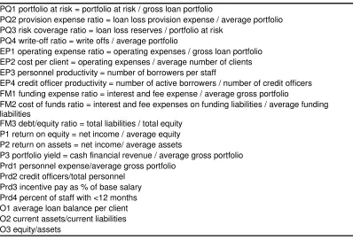
These are grouped in terms of portfolio quality, efficiency and productivity, financial management, profitability, productivity and others. Table 2 shows the values of these ratios in 30 Latin American MFIs.

Table 1 and Table 2 about here

The efficiency/productivity ratios reflect “how efficiently an MFI is using its resources, particularly its assets and personnel” (CGAP, 2003). Thus, efficiency ratios compare a measure of personnel employed with a measure of assets. Institutions can choose as assets either average gross loan portfolio, or average total assets, or average performing assets. CGAP describes as performing assets “loans, investments, and other assets expected to produce income”. Personnel may be defined as the total number of staff employed or the number of loan officers. In this paper we are going to use a different definition of efficiency, based on DEA, and we will compare traditional ratio based measures with DEA efficiencies. It will be shown that they are not the same thing, and that ratio analysis is no substitute for efficiency analysis as defined by the micro economic theory of production functions.

DEA efficiency and financial institutions

and Ravisankar (2000), Seiford and Zhu (1999), and Worthington (2004). The literature continues to grow all the time.

One advantage of DEA (nonparametric) over parametric approaches to measure efficiency is that this technique can be used when the conventional cost and profit functions cannot be justified; Berger and Humphrey (1997). DEA performs multiple comparisons between a set of homogeneous units. For an introduction to the theory of DEA see Thanassoulis (2001), Charnes et al. (1994), or Cooper et al. (2000).

For the purposes of this paper, it will be useful to make a distinction between model and specification in a DEA context. Different philosophical approaches as to what a financial institution does, and what is meant by efficiency lead to different models; see Berger and Mester (1997) for a full discussion. Two basic models are prevalent in the literature: intermediation and production; Athanassoupoulos (1997). Specification will refer to a more restricted concept: the particular set of inputs and outputs that enter into model definition.

Under the intermediation model, financial institutions collect deposits and make loans in order to make a profit. Deposits and acquired loans are considered to be inputs. Institutions are interested in placing loans, which are traditional outputs in studies of this kind; see, for example Berger and Humphrey (1991). Under the production model, a financial institution uses physical resources such as labour and plant in order to process transactions, take deposits, lend funds, and so on. In the production model manpower and assets are treated as inputs and transactions dealt with -such as deposits and loans- are treated as outputs. See, for example, Vassiloglou and Giokas (1990), Schaffnit et al. (1997), Soteriou and Zenios (1999).

and had to be excluded as a possible variable in the data set since the technique to be applied, DEA, requires homogeneous data for all the MFIs. Many MFIs obtain funds from the market (loans) or receive grants. Other issues become relevant in the selection of inputs and outputs. For example, some MFI receive subsidised loans at an interest rate that is below the market.

It follows that the selection of inputs and outputs is crucial in the financial institution modelling. Berger and Humphrey (1997) suggest that one could assess efficiency under a variety of output/input specifications, and see the way in which calculated efficiencies change as the specification changes. This is sensible, but they do not provide guidelines on how to choose between specifications. In fact, specification searches are common in the modelling of financial institutions; examples are Oral and Yolalan (1990), Vassiloglou and Giokas (1990), and Pastor and Lovell (1997).

A major problem with the selection of inputs and outputs in a DEA model is that there is no statistical framework on which significance tests can be based. The neat approach of variable selection that is used in regression, based on t statistic values, has no parallel in DEA. One may be tempted to use as many inputs and outputs as one may think to be relevant, but some of them will be correlated, perhaps highly so. Parkin and Hollingsworth (1997) review the problems that variable selection creates in DEA. Jenkins and Anderson (2003) warn against the use of correlated inputs and outputs in a DEA model. An important issue is that the number of 100% efficient units increases with the number of inputs and outputs in the model, and adding irrelevant variables may change the results obtained; Dyson et al. (2001), Pedraja Chaparro et al. (1999). Specification search methods in DEA have been proposed by Norman and Stocker (1991), Pastor et al. (2002), and Serrano Cinca and Mar Molinero (2004).

bivariate statistical analysis which throws light on the similarity between models, extreme observations, and the reasons why a particular MFI achieves a particular level of efficiency with a particular specification. This will be discussed in detail in the empirical example presented below.

Microfinance in Latin America

Most of the research on banking efficiency has concentrated on US and developed countries. So far, neither DEA nor other parametric or non-parametric frontier techniques have been used to evaluate the efficiency of microfinance institutions. Here we depart from this trend, and analyse thirty Latin American MFIs from Bolivia, Colombia, Dominican Republic, Ecuador, Mexico, Nicaragua, Peru and Salvador. Some of them are for profit institutions and others are not profit oriented. Some MFIs are just specialised banking institutions, while others are Non-Governmental Organisations (NGOs). The question arises of whether this difference influences efficiency, or the way in which efficiency is achieved.

According to Miller (2003), some of the most experienced, developed, and diverse MFIs around the world can be found in Latin America. Using 2001 and 2002 data from 124 worldwide MFIs (provided by the MicroBanking Bulletin), almost half of them from Latin America, the author draws several conclusions: MFIs from this region have more assets, are more leveraged, and make use of an increasingly growing share of commercial funds than institutions from other regions. Lapenu and Zeller (2002) complete this vision: comparing African, Asian and Latin America MFIs, they find that the number of institutions and the number of clients remain small in Latin American MFIs compared to Asian. However, Latin American MFIs mobilise a good amount of savings and loans in comparison to Asian MFIs. Finally, Latin America records the largest volume per transaction although rural outreach remains low.

the data is measured in monetary units (thousand of dollars), except the number of credit officers and the number of loans outstanding.

Selection of inputs and outputs

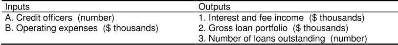
The selection of inputs and outputs in the model was based on Yaron’s (1994) outreach and sustainability framework. The number of loans outstanding (output) and the gross loan portfolio (output) were selected as measures of outreach. The two aspects of sustainability, operational and financial, guided the selection of a further input and output. Interest and fee income (output) was taken as an indicator of operational sustainability, as a MFI that fails to collect enough income is not viable in the long term. Financial sustainability was captured through operating expenses. In essence, the collection of fee and interest income is necessary for survival, but such survival cannot be long lasting if this income is collected at high cost. In common with other similar studies, the number of credit officers was also used as an input.

The inputs selected in this study are credit officers and operating expenses. A production model would suggest the inclusion of the first input, while the second input is consistent with an intermediation model. Jansson et al. (2003) define loan officers as “ personnel whose main activity is direct management of a portion of the loan portfolio” . Our choice of input could have been total staff, but this would have included people whose activity is unrelated to the MFI activity. The number of employees has been proposed as an input by Berger and Humphrey (1997), Dekker and Post (2001), Desrochers and Lamberte (2003), Leon (1999), and Tortosa-Ausina (2001) among others. Operating expenses –or similar inputs have been suggested by Berger and Humphrey (1997), Cuadras-Morató et al. (2001), Laeven (1999), Pastor (1999) and Worthington (1998). Operating expenses are “ expenses related to the operation of the institution, including all the administrative and salary expenses, depreciation and board fees” ; Jansson et al. (2003).

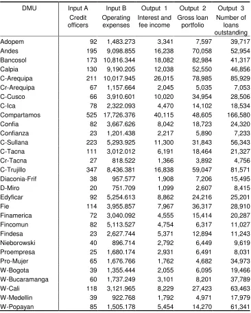
intermediation orientation, whereas the number of loans outstanding is associated with a production orientation. We wish to emphasize that the gross loan portfolio and the number of loans outstanding appeared as components of MFI efficiency ratios in Table 1. Interest and fee incomes are used by Pastor (1999). Gross loan portfolio or similar measures are often mentioned: Berger and Humphrey (1997), Desrochers and Lamberte (2003), Laeven (1999), Lozano-Vivas (1998), Leon (1999), Tortosa-Ausina (2001), and Worthington (1998). Finally, the number of loans outstanding is mentioned by Berger and Humphrey (1997), Budnevich et al. (2001) and Tortosa-Ausina (2001). As there is some difficulty in getting data for the number of loans processed in a given period, we use instead the stock of loans. Table 4 gives the values of inputs and outputs for the MFIs in the sample1.

Table 3 about here

Table 4 about here

Specifications and DEA efficiencies

to gross loan portfolio, contained in the list recommended by the consensus group of rating agencies, donors, banks, and voluntary organizations.

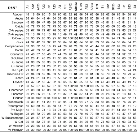
Other views of the way in which a MFI operates can be generated by using different combinations of inputs and outputs. Efficiency ratios are a particular case obtained when only one input and only one output enter into the specification. It is, of course, possible to think of all possible combinations of inputs and outputs. The total number of possible specifications with two inputs and three outputs is 21. The complete list of specifications can be seen in Table 5.

DEA efficiencies for each MFI were calculated using the CCR model of constant returns to scale; Charnes, Cooper, and Rhodes (1978). The results are given in Table 5.

Table 5 about here

Visual examination of Table 5 reveals some important features. Two MFIs (W-Popayan, an NGO and Findesa, a non-bank financial institution) are 100% efficient under many specifications. On the other side, some MFI achieve low scores under most specifications. No MFI is efficient under all specifications, highlighting the fact that the selection of inputs and outputs and, therefore, the view of what constitutes efficiency in this sector is a matter of importance. If we take, for example, W-Popayan, we find that it is 100% efficient under 18 specifications, meaning that it is an excellent institution, but its efficiency drops below 30% under A1, A2 and A12. We conclude that W-Popayan is good in any specification that contains either input B or output 3, indicating that this MFI is good at generating lots of loans with low operating expenses. A counter example is Fie, a non-bank financial institution, whose scores tend to be low, but becomes 100% efficient under 4 specifications: AB12, AB123, AB2, AB23. This indicates that, although Fie can take action to improve its efficiency, it has some strong points that deserve further attention.

addition, if two MFIs achieve the same efficiency score under a given specification they may do so following very different patterns of behaviour: there is no single path to efficiency in MFI. Exploring what is behind a DEA score is the objective of the next sections.

Multivariate analysis of DEA efficiency results

Serrano Cinca and Mar Molinero (2004) propose a specification search methodology based on treating the data in Table 5 as a multivariate data set. Other examples of the use of this approach are Serrano Cinca et al. (2004a), and Serrano Cinca et al. (2004b). This involves treating specifications as variables and MFIs as cases in a Principal Components Analysis (PCA). For an account of PCA see, for example, Chatfield and Collins (1980).

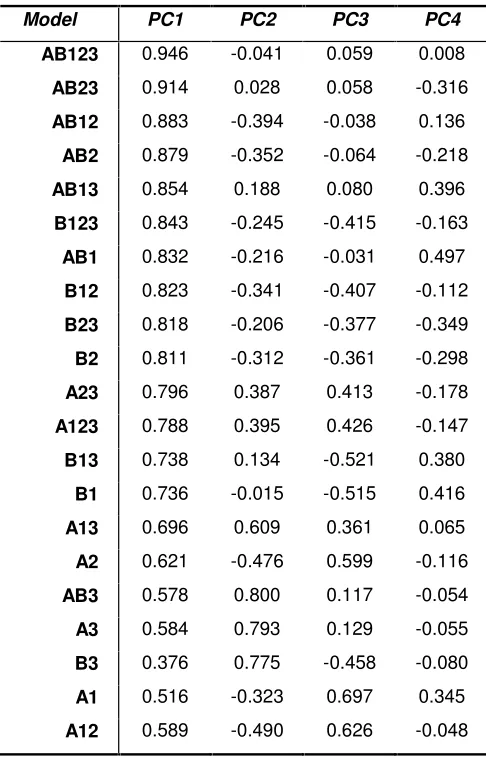
The first principal component, accounting for 57% of the variance, has an associated eigenvalue of 12.1; the second component accounts for a further 18% of the variance with an associated eigenvalue of 3.8; the third component, in turn accounts for 15% of the variance with an eigenvalue of 3.1; finally, there is only one more eigenvalue greater than 1, at 1.3, accounting for 6.4% of the variance. In total, the first four principal components account for 97% of the variance. This suggests that only four numbers (components) are required to explain why a particular MFI achieves a certain level of efficiency under all specifications.

components 1 and 2 can be seen in Figure 1, and component loadings in principal components 2 and 3 can be seen in Figure 2.

Table 6 about here

Figure 1 about here

Figure 2 about here

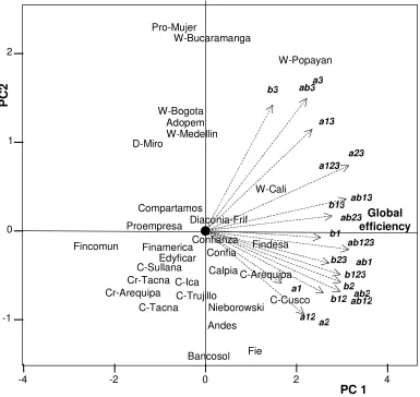
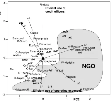
If we look at Figure 1 while taking into account the numbers in Table 5, some interesting features appear. W-Popayan, Findesa, C-Cusco, that are efficient under many specifications, appear at the right hand side of the figure. At the other extreme of the figure we find MFIs such as Cr-Arequipa and Fincomun, that achieve low levels of efficiency under most specifications. This is in line with our observation that the first principal component provides an overall rating in terms of efficiency. We could approach the understanding of the remaining components in a similar vein. For example, the second component appears to be associated with Non-Governmental Organisation (NGO) status, as all the MFIs with a positive score in this component are NGOs, and all the MFIs with a negative value of the component, with the exception of Nieborowski, are non-NGOs. Towards the top of Figure 2 we find MFIs whose efficiency is higher under specifications that contain input A (credit officers) than under specifications that contain input B (operating expenses). The most extreme example is Findesa. Findesa is 100% efficient under all models that contain input A, but its efficiency drops considerably when this input is excluded. This would suggest that the third principal component is associated with the efficient use of input A versus the efficient use of input B. However, it is dangerous to perform this type of labelling exercise without the help of a formal tool. In order to interpret the meaning of the components and in order to highlight the information contained in the figures, we resort to the technique of Property Fitting (Pro-Fit).

particular characteristic of a MFI is taken as a property. A line is drawn pointing in the direction towards the value of the property increases. For example, in Figure 1, if we calculate the efficiency of the various MFIs under specification B3, we find that W-Popayan is associated with the highest value, while Fincomun and Bancosol show the lowest values. B3 efficiency takes intermediate values in the remaining MFIs, increasing as we approach W-Popayan and decreasing as we approach Bancosol. Thus, a line from the origin towards W-Popayan, and away from Bancosol, would provide an indication of how B3 efficiency changes within Figure 1. A good introduction to Pro-Fit can be found in Schiffman et al. (1981). For some examples of the use of Pro-Fit within a management science context see Mar Molinero and Serrano Cinca (2001) and Serrano Cinca et al (2004a).

Pro-Fit lines have been calculated for all the specifications and displayed in Figures 1 and 2. Goodness of fit statistics associated with the Pro-Fit lines is given in Table 7. Figures 1 and 2 will now be interpreted in the light of the information contained in the directional vectors.

Table 7 about here

The first principal component has already been identified as an overall measure of efficiency that summarises all the models. This can be clearly seen in Figure 1, where all the lines associated with the different specifications are at acute angles with the horizontal axis, indicating positive correlation between the value of the first component score for each MFI and efficiency, in whatever specification efficiency is measured. In Figure 1, the label “ global efficiency” has been attached to the first component.

The second principal component has been already interpreted as being related to NGO status, and this is clear in Figure 2 where the shaded area contains all the MFIs with NGO status.

input B in their definition are associated with downward pointing directional vectors. The third principal component clearly reflects the different strategies followed by MFIs in their search for efficiency, opposing those that follow a policy of being efficient in the use of credit officers- positive values of the third principal component- and those that follow a policy of being efficient in their operating expenses – negative values of the third principal component. In Figure 2 we also see that Findesa can be considered to be a discordant observation. Indeed, Findesa is an extreme case of performance related pay, since 99% of credit officers’ salary is due to incentive pay, and this is reflected in our results.

Principal Component 4 was found to be associated with input 2- gross loan portfolio. Specifications that contain output 2 in their definition produce vectors that point towards the negative end of the fourth principal component, while specifications that exclude this output produce vectors that point towards the positive side. This is sending the message that the inclusion or exclusion of this output affects efficiency values.

In summary, when describing a MFI from the point of view of efficiency, we need to refer to at least four characteristics, or principal components of efficiency. The first principal component refers to an overall assessment of efficiency under all possible models, and gives a ranking of MFIs. The second component refers to the NGO status. The third principal component is associated with inputs and reveals which MFIs have an approach to efficiency based on credit officers, and which ones approach efficiency by concentrating on operating expenses. The fourth principal component is associated with the inclusion or exclusion of an output in the model: gross loan portfolio.

3 where the difference appears most clearly. W-Popayan is at the bottom of Figure 2 indicating efficient use of credit officers, while Findesa is located towards the top of the same figure, indicating efficient use of operating expenses. Both W-Popayan and Findesa achieve similar scores with respect to Principal Component 4.

Non-governmental organisations and country effect

Two aspects of MFIs will now be examined: their country of operation, and their non-governmental (NGO) status. We will start with the NGO status.

Given the aims and objectives of MFIs - the fight against poverty, self-help, and the promotion of women’s status -, it is not surprising to discover that many of them are NGOs. In fact, very often an organisation starts as an NGO, and when it becomes well established in the microfinance world, changes into a non-banking financial institution. But are NGOs more or less efficient than non-NGOs MFIs? Is there anything in the way they achieve efficiency that distinguishes them?

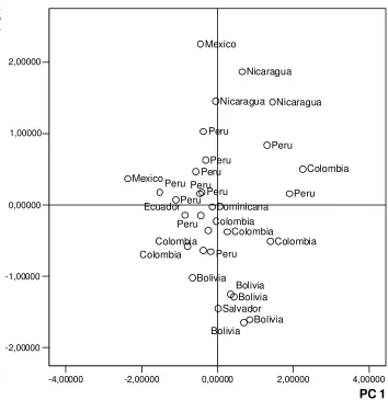
We now turn our attention to the country effect. There is a country effect, best seen in Principal Component 4. Figure 3 plots component scores in principal component 1 versus principal component 4. The names of the MFIs have been replaced with the names of the countries in which MFIs operate. We can see that there is very little overlap between the countries. From top to bottom, all Nicaraguan MFIs appear together; all but one Peruvian MFIs appear together; all but one Colombian MFIs appear together; and all Bolivian MFIs appear together. Nothing can be said about Salvador, Ecuador, and the Dominican Republic, since these countries are represented by just one MFI each. There is no right to left grouping of countries in Figure 3, indicating that country of origin and overall efficiency are unrelated. Remembering that Principal Component 4 is associated with output 2 (gross loan portfolio), one would conclude that efficiency of MFIs in Bolivia is associated with building large portfolios, while efficiency of MFIs in Nicaragua has to be assessed in terms of the number of loans or the amount of interests and fees collected by the MFI. In fact, Bolivia has one of the more developed microfinance markets, where margins are narrowing and this is resulting in mergers and acquisitions within the MFI industry, Silva (2003).

Figure 3 about here

DEA efficiency and ratio analysis

Up to now we have been working with DEA efficiency. We have been able to rate MFIs in terms of overall DEA efficiency; we have seen that there are effects associated with NGO status; and we have observed country effects. The question remains of what the DEA analysis adds to our knowledge of microfinance institutions? Have we observed effects that would have remained hidden if we had used traditional ratio analysis? This will be the object of the current section.

It is clear that there is redundancy in a set of 21 ratios, and that it should be possible to use a smaller number of factors in order to describe what is special about a given MFI. For this reason, ratios have been treated as variables and MFIs as observations and principal component analysis has been performed. Seven principal components were found to be associated with eigenvalues greater than one, accounting for 79% of the total variance in the data.

We have now reasoned as follows. Seven factors are needed to describe a MFI from the point of view of ratio analysis. Some of these factors are probably related to efficiency, in whatever form this is defined. Indeed, ratios EP1 to EP4 are known in the trade as “ efficiency and productivity ratios” . If efficiency is captured by the ratios, there will be at least one principal component that reflects efficiency. Of course, this definition of efficiency does not have to coincide with DEA efficiency, but one expects that if a MFI is efficient from the point of view of ratio analysis, it will also be efficient from the DEA point of view. The fact that some DEA specifications coincide with ratio definitions make us think that the two approaches will be related. But in this paper we have shown how to define a measure of overall efficiency taking into account all possible specifications. Does ratio analysis capture in any way such measure of overall efficiency?

To answer this question we have computed Pearson correlation coefficients between component scores obtained from the ratios in Table 2, and principal components obtained from efficiency scores in Table 5. These are summarised in Table 8.

Table 8 about here

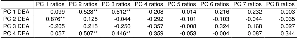
country effect, is correlated with the second and the third principal components of the ratios. If we look at component correlations, not shown here, we find that the first principal component of the ratios is correlated with EP3 (number of borrowers per staff), EP4 (number of borrowers per credit officer), FM3 (debt/equity ratio), O1 (average loan balance per client) and O3 (equity/assets ratio); the second principal component of the ratios is correlated with EP1 (operating expense ratio), FM1 (funding expense ratio), FM2 (cost of funds ratio), and Prd1(Personnel expense/average gross portfolio). Of all efficiency ratios, only EP1 appears to be associated with the overall measure of DEA efficiency, and its effect is relatively low, as the correlation of EP1 with the first principal component of the ratios is 0.75, and the correlation of the second principal component of the ratios with the first principal component of DEA efficiencies is -0.53. We have to conclude that efficiency and productivity ratios are only vaguely related to efficiency from the DEA point of view. What are we to conclude? DEA efficiency is well based on Economic Theory, while ratios are only consensus indicators. Everyone can make up his/her own mind, but we lean towards DEA efficiency.

Conclusions

DEA has long been applied to the measurement of financial institutions efficiency. Here we have used it to assess efficiency of MFIs, which have a banking side and a social side. We have suggested a methodological approach that goes behind a DEA measure and explains the scores obtained under different choices of models and specifications.

We have obtained DEA efficiencies for every combination of inputs and outputs of 30 Latin American MFIs. This way, we can see that the level of efficiency achieved by a MFI depends on the specification chosen. So the choice of a particular model or specification is relevant for efficiency assessment.

understand why a MFI achieves a level of efficiency under a given specification, or which are the paths to efficiency followed by a group of MFIs.

Finally, there is no reason why we should be fanatic believers in a DEA efficiency world, but the converse is also true. Efficiency and productivity ratios that have emerged from the deliberations of a committee need not be associated with efficiency nor with productivity. We have shown that our approach to efficiency analysis not only produces an overall ranking of MFIs in terms of the use they make of inputs and outputs, but also reveals features that distinguish NGOs from non-NGO institutions, that we can explain the reasons why some MFIs are or are not efficient, and that there are country effects in the data.

References

Athanassopoulos, A. D. (1997): Service quality and operating efficiency synergies for management control in the provision of financial services: Evidence from Greek bank branches. European Journal of Operational Research, 98, 300-313

Bala, K. and Cook, W. D. (2003) Performance measurement with classification information: an enhanced additive DEA model. Omega, 31, (6), 439-450

Berger, A.N., and Humphrey, D.B. (1991): The dominance of inefficiencies over scale and product mix economies in banking. Journal of Monetary Economics, 28, 117-148 Berger, A. N. and Humphrey, D. B. (1997): Efficiency of financial institutions: International survey and directions for future research. European Journal of Operational Research 98, 175-212

Berger, A.N., and Mester, L.J. (1997): Inside the black box: what explains differences in the efficiencies of financial institutions? Journal of Banking and Finance, 21, 895-947 Brockett, P.L.; Cooper W.W.; Golden L.L.; Rousseau J.J.; and Wang Y.Y. (2004): Evaluating solvency versus efficiency performance and different forms of organization and marketing in US property - liability insurance companies. European Journal of Operational Research, 154 (2), 492-514

CGAP (2001): Resource Guide to Microfinance Assessments. CGAP Focus Note nº 22, Washington D.C., Consultative Group to Assist the Poorest

CGAP (2003): Microfinance consensus guidelines. Definitions of selected financial terms, ratios and adjustments for microfinance, 3rd edition. Washington D. C., Consultative Group to Assist the Poorest

Charnes, A.; Cooper, W. W. and Rhodes, E. (1978): Measuring the efficiency of decision making units. European Journal of Operational Research, 2, 429-444

Charnes, A.; Cooper, W.W.; Lewin, Y.A.; and Seiford, M.L. (Eds) (1994): Data Envelopment Analysis: theory, methodology, and applications. Kluwer Academic Publishers

Chatfield, C.; and Collins, A.J. (1980): Introduction to multivariate analysis. Chapman and Hall. London. UK

Chaves, R. and González-Vega, C. (1996): The design of successful financial intermediaries: evidence from Indonesia. World Development, 24, (1), 65-78

Cuadras-Morató, X. Fernández Castro, A. and Rosés, J. R. (2001): Productividad, Competencia e Innovación en la Banca Privada Española (1900-1914), Economic working paper 364, Department of Economics and Business, Universitat Pompeu Fabra, Spain

Daley-Harris, S. (2003): State of the Microcredit Summit Campaign Report 2003, Microcredit Summit Campaign, Washington D. C.

Dekker, D. and Post, T. (2001): A quasi-concave DEA model with an application for bank branch performance evaluation. European Journal of Operational Research, 132, 296-311

Desrochers, M.; and Lamberte, M. (2003): Efficiency and Expense Preference in Phillippines’s Cooperative Rural Banks. Working paper 03-21 CIRPÉE (Centre Interuniversitaire sur le risque, les politiques économiques et l’emploi), Québec, Canada Dyson, R.G.; Allen, R.; Camanho, A.S.; Podinovski, V.V.; Sarrico, C.S.; and Shale, E.A. (2001): Pitfalls and protocols in DEA. European Journal of Operational Research, 132, 245-259

Hartman, T. E.; Storbeck, J. E. and Byrnes, P. (2001): Allocative efficiency in branch banking. European Journal of Operational Research, 134, 232-242

Hollis, A. and Sweetman, A. (1998): Microcredit: What Can we Learn form the Past? World Development, 26, (10) 1875-1891

Jansson, T. et al. (2003): Performance indicators for microfinance institutions. Technical Guide, 3rd _{edition, Microrate and Inter-American Development Bank,} Washington D.C.

Jenkins, L.; and Anderson, M. (2003): A multivariate statistical approach to reducing the number of variables in data envelopment analysis. European Journal of Operational Research, 147, 51-61

Johnson, S.; and Rogaly, B. (1997): Microfinance and Poverty Reduction. Oxford and London, Oxfam and ACTIONAID

Kuosmanen, T. and Post, T. (2001): Measuring economic efficiency with incomplete price information: with an application to European commercial banks. European Journal of Operational Research, 134, 43-58

Laeven, L. (1999): Risk and Efficiency in East Asian Banks, 2255 Research on Financial Domestic System Working Paper, World Bank, Washington D. C.

Leon, J. (1999): Eficiencia en costos en los bancos comerciales de México: una aplicación de la aproximación no paramétrica DEA, unpublished paper presented at the Latin American Econometric Association Meeting, Cancún, México

Lozano-Vivas, A. (1998): Efficiency and technical change for Spanish banks. Applied Financial Economics, 8, 289-300

Luo, X. (2003): Evaluating the profitability and marketability efficiency of large banks: An application of data envelopment analysis. Journal of Business Research, 56, (8), 627-635

Mar Molinero, C.; and Serrano Cinca, C. (2001): Bank failure: a multidimensional scaling approach. European Journal of Finance, 7, 165-183

Miller, J. (2003): Benchmarking Latin America microfinance [on line] microfinancegateway.org

<http://www.microfinancegateway.org/content/article/detail/3820> (16/01/04)

Morduch, J. (1999): The microfinance promise. Journal of Economic Literature, 37, 1569-1614

Navajas, S.; Schreiner, M.; Meyer, R. L.; González-Vega, C.; and Rodríguez-Meza, J. (2000): Microcredit and the poorest of the poor: Theory and Evidence from Bolivia. World Development, 28, (2), 333-346

Norman, M.; and Stocker, B. (1991): Data Envelopment Analysis: the assessment of performance. John Wiley and Sons, Chichester, UK

Oral, M., and Yolalan, R. (1990): An Empirical Study on Measuring Operating Efficiency and Profitability of Bank Branches. European Journal of Operational Research, 46, 282-294

Paradi, J. C. and Schaffnit, C. (2003): Commercial branch performance evaluation and results communication in a Canadian bank––a DEA application. European Journal of Operational Research, 156 (3), 719-735

Parkin, D.; and Hollingsworth, B. (1997): Measuring production efficiency of acute hospitals in Scotland, 1991-94: validity issues in data envelopment analysis. Applied Economics, 29, 1425-1433

Pastor, J. M. (1999): Efficiency and risk management in Spanish banking: a method to descompose risk Applied Financial Economics, 9, 371-384

Pastor, J.M., and Lovell, C.A.K. (1997): Target setting in a bank branch network. European Journal of Operational Research, 98, 290-299

Pastor, J. M., Ruiz Gomez, J.L. and Sirvent, I. (2002): A statistical test for nested radial DEA models. Operations Research, 50 (4), 728-735

Pedraja Chaparro, F.; Salinas Jimenez, J., and Smith, P. (1999): On the quality of Data Envelopment Analysis model. Journal of the Operational Research Society, 50, 636-645

Pille, P. and Paradi, J. C. (2002): Financial performance analysis of Ontario (Canada) Credit Unions: An application of DEA in the regulatory environment. European Journal of Operational Research, 139, (2), 339-350

Saha, A., and Ravisankar, T.S. (2000): Rating of Indian commercial banks: A DEA approach. European Journal of Operational Research, 124, 187-203

Schaffnit, C., Rosen, D. and Paradi, J. (1997): Best practice analysis of bank branches: An application of DEA in a large Canadian bank. European Journal of Operational Research, 98, 269-289

Schiffman, S.S.; Reynolds, M.L.; and Young, F.W. (1981): Introduction to Multidimensional Scaling: Theory, Methods and Applications. Academic Press, London Schreiner, M. and Yaron, J. (2001): Development Finance Institutions. Measuring their subsidy. The World Bank, Washington D. C.

Seiford, L.M. and Zhu, J. (1999): Profitability and marketability of the top 55 U.S. commercial banks. Management Science, 45 (9), 1270-1288

Serrano Cinca, C.; and Mar Molinero, C. (2004): Selecting DEA specifications and ranking units via PCA. Journal of the Operational Research Society, 55, 521-528 Serrano Cinca, C.; Mar Molinero, C.; and Chaparro, F. (2004a): Spanish savings banks: a view on intangibles. Knowledge Management Research and Practice. Forthcoming Serrano Cinca, C.; Fuertes Callen, Y.; and Mar Molinero, C. (2004b): Measuring DEA efficiency in Internet companies. Decision Support Systems. Forthcoming

Silva, S. (2003): Microfinance institutions win a coveted seal of approval, Microenterprise Americas, 12-17

Soteriou, A. and Zenios, S.A. (1999): Operations, quality and profitability in the provision of banking services. Management Science, 45 (9), 1221-1238

Thanassoulis, E. (2001): Introduction to the theory and application of data envelopment analysis. Kluwer Academic Publishers, Dordrecht, The Netherlands

Vassiloglou, M. and Giokas, D. (1990): A study of the relative efficiency of bank branches: An application of data envelopment analysis. The Journal of the Operational Research Society, 41, 591-597

Von Pischke, J. D. (2002): Microfinance in Developing Countries. In: Carr, J. H. y Tong, Z. Y. (Eds) Replicating Microfinance in the United States, Washington: Woodrow Wilson Center Press, 65-96

Worthington, A. (1998): The determinants of non-bank financial institution efficiency: a stochastic cost frontier approach. Applied Financial Economics, 8, 279-287

PQ1 portfolio at risk = portfolio at risk / gross loan portfolio

PQ2 provision expense ratio = loan loss provision expense / average portfolio PQ3 risk coverage ratio = loan loss reserves / portfolio at risk

PQ4 write-off ratio = write offs / average portfolio

EP1 operating expense ratio = operating expenses / gross loan portfolio EP2 cost per client = operating expenses / average number of clients EP3 personnel productivity = number of borrowers per staff

EP4 credit officer productivity = number of active borrowers / number of credit officers FM1 funding expense ratio = interest and fee expense / average gross portfolio

FM2 cost of funds ratio = interest and fee expenses on funding liabilities / average funding liabilities

FM3 debt/equity ratio = total liabilities / total equity P1 return on equity = net income / average equity P2 return on assets = net income/ average assets

P3 portfolio yield = cash financial revenue / average gross portfolio Prd1 personnel expense/average gross portfolio

Prd2 credit officers/total personnel Prd3 incentive pay as % of base salary Prd4 percent of staff with <12 months O1 average loan balance per client O2 current assets/current liabilities O3 equity/assets

Table 1. The 21 ratios and their definitions

DMU PQ1 PQ2 PQ3 PQ4 EP1 EP2 EP3 EP4 FM1 FM2 FM3 P1 P2 P3 Prd1 Prd2 Prd3 Pr4 O1 O2 O3 Adopem 0.037 0.02 1.025 0.002 0.155 387.789 226 431 0.047 0.136 0.8 0.007 0.003 35.7 0.076 0.526 0.8 0.229 191 4.7 0.509 Andes 0.06 0.035 1.161 0.014 0.137 189.492 69 248 0.026 0.054 10 0.33 0.03 0.258 0.087 0.276 0.237 0.162 1451 1.9 0.086 Bancosol 0.12 0.045 0.726 0.013 0.132 210.876 74 239 0.028 0.054 5.6 0.049 0.007 0.223 0.068 0.311 0.389 0.222 2008 2.1 0.148 Calpia 0.031 0.034 1.393 0.003 0.19 205.556 136 360 0.018 0.04 5 0.17 0.028 0.276 0.091 0.377 0.41 0.27 1122 1.9 0.143 C-Arequipa 0.061 0.032 1.122 0.005 0.135 148.869 129 336 0.037 0.064 5.2 0.547 0.08 0.393 0.073 0.384 0.11 0.231 1122 1.2 0.148 Cr-Arequipa 0.057 0.034 0.99 0.011 0.248 203.063 48 91 0.058 0.127 4.2 0.264 0.054 0.487 0.134 0.526 0.5 0.447 825 5.7 0.187 C-Cusco 0.048 0.015 1.173 0.001 0.123 1560.900 129 400 0.031 0.054 5.2 0.593 0.085 0.356 0.073 0.323 0.11 0.157 1333 1.2 0.155 C-Ica 0.169 0.001 0.876 0 0.173 1500.884 91 237 0.041 0.077 3.9 0.325 0.058 0.349 0.091 0.385 0 0.291 761 1.3 0.193 Compartamos 0.01 0.028 5.128 0 0.391 113.787 182 317 0.064 0.155 1.7 0.61 0.21 1.016 0.262 0.573 0.5 0.421 292 2.8 0.341 Confia 0.017 0.054 1.644 0 0.217 1909.873 99 256 0.075 0.132 6.3 0.498 0.059 0.49 0.125 0.385 0.65 0.296 890 1.3 0.13 Confianza 0.048 0.053 0.863 0.018 0.235 2090.002 133 287 0.06 0.108 4.2 0.181 0.036 0.513 0.113 0.463 0.12 0.244 894 3.5 0.182 C-Sullana 0.87 0.022 0.993 0.017 0.182 99.262 83 253 0.061 0.111 5.2 0.352 0.055 0.42 0.083 0.328 0.12 0.308 565 1.4 0.154 C-Tacna 0.061 0.012 0.883 0.001 0.167 169.844 61 166 0.062 0.092 5.2 0.316 0.052 0.398 0.079 0.366 0.123 0.26 1004 1.3 0.154 Cr-Tacna 0.094 0.007 0.941 0.01 0.223 2026.796 74 166 0.039 0.091 2.9 0.216 0.051 0.39 0.13 0.444 0 0.244 904 3.2 0.241 C-Trujillo 0.052 0.028 0.94 0 0.159 134.940 68 192 0.038 0.074 5.8 0.441 0.067 0.367 0.079 0.354 0.054 0.326 885 1.3 0.141 Diaconia-Frif 0.155 0.059 0.38 0.001 0.142 65.232 194 408 0 0 0 0.062 0.06 0.297 0.086 0.475 0 0.288 465 48.8 0.982 D-Miro 0.009 0.016 1.885 0 0.322 97.713 157 421 0.019 0.062 0.6 0.171 0.119 0.607 0.186 0.374 0.64 0.505 310 2.3 0.581 Edyficar 0.075 0.022 0.851 0.051 0.226 214.961 92 274 0.037 0.097 3 0.205 0.047 0.399 0.137 0.335 0.076 0.36 961 1.8 0.233 Fie 0.069 0.058 1.263 0.015 0.114 149.430 98 242 0.027 0.063 6.3 0.156 0.021 0.24 0.065 0.405 0.515 0.3 1318 2.5 0.13 Finamerica 0.113 0.02 0.29 0.004 0.198 165.682 90 257 0.046 0.083 5.9 -0.36 -0.049 0.271 0.103 0.350 0.144 0.228 833 1.3 0.136 Fincomun 0.036 0.023 1.004 0.016 0.849 502.138 54 134 0.074 0.073 3.7 -0.019 -0.003 0.934 0.565 0.398 0.67 0.301 573 1.4 0.196 Findesa 0.02 0.034 0.87 0.005 0.224 265.590 114 489 0.094 0.203 4.2 0.152 0.032 0.506 0.139 0.232 0.99 0.242 1147 14.5 0.187 Nieborowski 0.036 0.039 0.729 0.005 0.151 1011.806 97 239 0.038 0.08 2.7 0.803 0.215 0.571 0.081 0.407 0.8 0.267 670 4.6 0.258 Proempresa 0.105 0.07 0.794 0.012 0.269 238.407 107 292 0.053 0.108 3.6 0.05 0.011 0.498 0.129 0.368 0.032 0.338 889 2.8 0.208 Pro-mujer 0.002 0.008 13.995 0.002 0.364 47.629 173 538 0.017 0.082 0.6 0.046 0.034 42.2 0.186 0.322 0 0.302 134 20.3 0.612 W-Bogota 0.021 0.022 0.866 0.006 0.248 79.032 210 479 0.058 0.142 2.9 0.035 0.01 0.41 0.128 0.438 0.414 0.348 327 2.4 0.252

W-Bucaramanga 0.008 0.012 1.008 0.002 0.241 510.437 296 629 0.067 0.143 2.9 0.039 0.011 0.449 0.114 0.471 0.509 0.388 218 2.2 0.249

W-Cali 0.012 0.014 2.576 0.002 0.126 57.969 260 497 0.047 0.144 1.7 0.184 0.071 0.346 0.07 0.524 0.3 0.311 468 2.6 0.356 W-Medellin 0.024 0.015 0.929 0.006 0.196 55.545 187 451 0.047 0.123 1.6 0.098 0.037 0.383 0.115 0.415 0.433 0.298 283 3.4 0.378 W-Popayan 0.01 0.006 1 0 0.115 274.482 354 724 0.03 0.16 0.6 0.247 0.16 0.433 0.062 0.489 0.78 0.038 233 5.5 0.629

Inputs Outputs

A. Credit officers (number) 1. Interest and fee income ($ thousands)

B. Operating expenses ($ thousands) 2. Gross loan portfolio ($ thousands)

3. Number of loans outstanding (number)

DMU Input A Credit officers Input B Operating expenses

Output 1 Interest and

fee income

Output 2 Gross loan

portfolio

Output 3 Number of

loans outstanding

Adopem 92 1,483.273 3,341 7,597 39,717

Andes 195 9,098.855 16,238 70,058 52,954

Bancosol 173 10,816.344 18,082 82,984 41,317

Calpia 130 9,190.205 12,038 52,550 46,856

C-Arequipa 211 10,017.945 26,015 78,985 85,929

Cr-Arequipa 67 1,157.664 2,045 5,035 7,053

C-Cusco 66 3,910.601 10,020 34,954 28,506

C-Ica 78 2,322.093 4,470 14,102 18,534

Compartamos 525 17,726.376 40,115 48,605 166,580

Confia 82 3,667.626 8,042 18,723 24,320

Confianza 23 1,201.438 2,217 5,890 7,233

C-Sullana 223 5,293.925 11,300 31,843 56,343

C-Tacna 111 3,012.012 6,191 18,464 21,327

Cr-Tacna 27 818.522 1,366 3,892 4,756

C-Trujillo 347 8,436.381 16,838 59,047 81,571

Diaconia-Frif 38 957.577 1,908 7,206 15,495

D-Miro 20 751.709 1,099 2,607 8,415

Edyficar 92 5,254.613 8,862 24,216 25,201

Fie 114 3,955.857 7,967 36,317 28,910

Finamerica 72 3,040.092 4,555 15,414 20,287

Fincomun 82 5,113.527 4,754 6,317 11,027

Findesa 23 2,627.744 5,371 12,894 11,243

Nieborowski 40 896.714 2,792 6,449 9,619

Proempresa 25 1,680.174 2,931 6,491 8,031

Pro-Mujer 65 1,676.766 1,762 4,682 34,973

W-Bogota 39 1,355.444 2,055 6,095 19,466

W-Bucaramanga 60 1,737.249 3,101 8,201 37,789

W-Cali 118 3,121.965 8,229 27,423 63,463

W-Medellin 39 922.768 1,792 4,971 17,979

W-Popayan 85 1,505.178 5,454 14,270 61,341

DMU

13 _B2 _B23 _B3

Adopem 16 16 60 60 15 60 60 62 62 66 66 54 66 66 62 62 66 66 54 66 66

Andes 36 64 64 48 64 64 38 66 85 85 66 85 85 38 49 81 81 49 81 81 14

Bancosol 45 86 86 47 86 86 33 67 90 90 67 90 90 33 46 81 81 46 81 81 9

Calpia 40 72 73 60 72 73 50 55 75 78 60 75 78 50 36 60 60 36 60 60 13

C-Arequipa 53 67 76 71 67 76 56 97 97 97 97 87 88 56 72 83 83 72 83 83 21

Cr-Arequipa 13 13 18 18 13 18 15 49 49 49 49 46 46 15 49 49 49 49 46 46 15

C-Cusco 65 95 95 80 95 95 60 100 100 100 100 100 100 60 71 94 94 71 94 94 18

C-Ica 24 32 42 39 32 42 33 64 66 66 64 66 66 33 53 64 64 53 64 64 20

Compartamos 33 33 52 52 16 45 44 78 78 78 78 30 45 44 62 62 62 62 29 29 23

Confia 42 42 53 53 41 52 41 81 81 81 81 56 57 41 61 61 61 61 54 54 16

Confianza 41 46 57 55 46 57 44 70 70 70 70 55 60 44 51 52 52 51 52 52 15

C-Sullana 22 26 41 40 26 41 35 66 66 66 66 65 65 35 59 63 63 59 63 63 26

C-Tacna 24 30 35 33 30 35 27 66 67 67 66 66 66 27 57 65 65 57 65 65 17

Cr-Tacna 22 26 32 31 26 32 25 56 56 56 56 52 52 25 46 50 50 46 50 50 14

C-Trujillo 21 30 41 37 30 41 32 62 75 75 62 75 75 32 55 74 74 55 74 74 24

Diaconia-Frif 22 34 63 59 34 63 56 63 81 81 63 81 81 56 55 79 79 55 79 79 40

D-Miro 24 24 61 61 23 61 58 52 52 61 61 38 61 58 40 40 40 40 37 37 27

Edyficar 41 47 52 50 47 52 38 65 65 65 65 51 56 38 47 49 49 47 49 49 12

Fie 30 57 57 43 57 57 35 70 100 100 70 100 100 35 56 97 97 56 97 97 18

Finamerica 27 38 50 45 38 50 39 55 56 56 55 56 56 39 41 53 53 41 53 53 16

Fincomun 25 25 26 26 14 22 19 37 37 37 37 14 22 19 26 26 26 26 13 13 5

Findesa 100 100 100 100 100 100 68 100 100 100 100 100 100 68 56 56 56 56 52 52 11

Nieborowski 30 30 41 41 29 41 33 94 94 94 94 77 77 33 86 86 86 86 76 76 26

Proempresa 50 50 59 59 46 58 44 71 71 72 72 48 60 44 48 48 48 48 41 41 12

Pro-Mujer 12 13 74 74 13 74 74 33 33 74 74 30 74 74 29 29 51 51 29 51 51

W-Bogota 23 28 72 70 28 72 69 53 53 72 70 49 72 69 42 47 47 42 47 47 35

W-Bucaramanga 22 24 87 87 24 87 87 59 59 87 87 51 87 87 49 50 53 53 50 53 53

W-Cali 30 41 82 78 41 82 74 84 95 95 84 95 95 74 73 93 93 73 93 93 50

W-Medellin 20 23 65 65 23 65 64 60 60 65 65 58 65 64 54 57 57 54 57 57 48

W-Popayan 28 30 100 100 30 100 100 100 100 100 100 100 100 100 100 100 100 100 100 100 100

Model PC1 PC2 PC3 PC4

AB123 0.946 -0.041 0.059 0.008 AB23 0.914 0.028 0.058 -0.316 AB12 0.883 -0.394 -0.038 0.136

AB2 0.879 -0.352 -0.064 -0.218

AB13 0.854 0.188 0.080 0.396 B123 0.843 -0.245 -0.415 -0.163

AB1 0.832 -0.216 -0.031 0.497

B12 0.823 -0.341 -0.407 -0.112

B23 0.818 -0.206 -0.377 -0.349

B2 0.811 -0.312 -0.361 -0.298

A23 0.796 0.387 0.413 -0.178

A123 0.788 0.395 0.426 -0.147

B13 0.738 0.134 -0.521 0.380

B1 0.736 -0.015 -0.515 0.416

A13 0.696 0.609 0.361 0.065

A2 0.621 -0.476 0.599 -0.116

AB3 0.578 0.800 0.117 -0.054

A3 0.584 0.793 0.129 -0.055

B3 0.376 0.775 -0.458 -0.080

A1 0.516 -0.323 0.697 0.345

A12 0.589 -0.490 0.626 -0.048

Model Directional cosines F Adj R2

J1 J 2 J 3 J 4

A1 0.09 -0.06 0.12 0.06 243.19 0.971

(16.30)** (-10.20)** (22.01)** (10.91)**

A12 0.14 -0.11 0.15 -0.01 330.95 0.978

(21.64)** (-18.00)** (22.99)** (-1.76)

A123 0.17 0.08 0.09 -0.03 307.00 0.977

(27.90)** (13.98)** (15.07)** (-5.21)**

A13 0.14 0.12 0.07 0.01 691.59 0.990

(36.79)** (32.20)** (19.09)** (3.46)*

A2 0.15 -0.11 0.14 -0.03 398.28 0.982

(24.98)** (-19.15)** (24.09)** (-4.68)**

A23 0.17 0.08 0.09 -0.04 432.07 0.983

(33.34)** (16.20)** (17.30)** (-7.44)**

A3 0.12 0.16 0.03 -0.01 620.98 0.988

(29.28)** (39.71)** (6.48)** (-2.74)

AB1 0.15 -0.04 -0.01 0.09 466.47 0.987

(36.18)** (-9.39)** (-1.34) (21.61)**

AB12 0.17 -0.08 -0.01 0.03 132.07 0.948

(20.77)** (-9.26)** (-0.89) (3.20)*

AB123 0.16 -0.01 0.01 0.00 55.93 0.883

(14.91)** (-0.64) (0.93) (0.13)

AB13 0.13 0.03 0.01 0.06 80.48 0.916

(15.91)** (3.50)* (1.49) (7.37)**

AB2 0.20 -0.08 -0.01 -0.05 112.06 0.939

(19.11)** (-7.65)** (-1.39) (-4.74)**

AB23 0.17 0.01 0.01 -0.06 97.85 0.930

(18.65)** (0.58) (1.18) (-6.46)**

AB3 0.12 0.16 0.02 -0.01 690.00 0.990

(30.52)** (42.22)** (6.18)** (-2.87)**

B1 0.11 0.00 -0.08 0.06 307.43 0.977

(26.07)** (-0.54) (-18.24)** (14.74)**

B12 0.16 -0.07 -0.08 -0.02 211.64 0.967

(24.29)** (-10.05)** (-12.01)** (-3.32)*

B123 0.15 -0.04 -0.08 -0.03 193.16 0.964

(23.79)** (-6.91)** (-11.73)** (-4.60)*

B13 0.11 0.02 -0.08 0.06 264.74 0.973

(24.28)** (4.40)* (-17.14)** (12.50)**

B2 0.17 -0.07 -0.08 -0.06 244.50 0.971

(25.69)** (-9.89)** (-11.44)** (-9.44)**

B23 0.17 -0.04)** -0.08 -0.07 258.94 0.973

(26.65)** (-6.72)** (-12.28)** (-11.38)**

B3 0.08 0.16 -0.09 -0.02 142.26 0.951

(9.15)** (18.89)** (-11.16)** (-1.95)

** Significant at the 0.01 level. * Significant at the 0.05 level

PC 1 ratios PC 2 ratios PC 3 ratios PC 4 ratios PC 5 ratios PC 6 ratios PC 7 ratios PC 8 ratios

PC 1 DEA 0.099 -0.528** 0.612** -0.208 -0.014 0.216 0.232 0.003

PC 2 DEA 0.876** 0.125 -0.044 -0.292 -0.101 -0.103 -0.044 -0.035

PC 3 DEA -0.205 0.215 -0.250 -0.357 -0.008 0.324 0.168 0.027

PC 4 DEA 0.057 0.507** 0.446** 0.359 -0.053 -0.004 0.087 0.344

** Significant at the 0.01 level (bilateral)

P

C

2

-4 -2 0 2 4

PC 1 -1 0 1 2 Adopem Andes Bancosol Calpia C-Arequipa Cr-Arequipa C-Cusco C-Ica Compartamos Confia Confianza C-Sullana C-Tacna Cr-Tacna C-Trujillo Diaconia-Frif D-Miro Edyficar Fie Finamerica Fincomun Findesa Nieborowski Proempresa Pro-Mujer W-Bogota W-Bucaramanga W-Cali W-Medellin W-Popayan a1 a12 a123 a13 a2 a23 a3 ab1 ab12 ab123 ab13 ab2 ab23 ab3 b1 b12 b123 b13 b2 b23 b3 Global efficiency

P

C

3

-1 0 1 2

-2 -1 0 1 2 3 Adopem Andes Bancosol Calpia C-Arequipa Cr-Arequipa C-Cusco C-Ica Compartamos Confia Confianza C-Sullana C-Tacna Cr-Tacna C-Trujillo Diaconia-Frif D-Miro Edyficar Fie Finamerica Fincomun Findesa Nieborowski Proempresa Pro-Mujer W-Bogota W-Bucaramanga W-Cali W-Medellin W-Popayan PC2 Efficient use of

credit officers

Efficient use of operating expenses

a1 a12 a123 a13 a2 a23 a3 ab1 ab12 ab123 ab13 ab2 ab23 ab3 b1 b12 b123 b13 b2 b23 b3

NGO

-4,00000 -2,00000 0,00000 2,00000 4,00000

PC 1

-2,00000 -1,00000 0,00000 1,00000 2,00000

P

C

4

Dominicana

Bolivia

Bolivia Salvador

Peru

Peru

Peru

Peru

Mexico

Nicaragua

Peru

Peru Peru Peru

Peru

Bolivia Ecuador

Peru

Bolivia Colombia

Mexico

Nicaragua Nicaragua

Peru

Bolivia

Colombia ColombiaColombia Colombia

Colombia

1_{Some of the data had to be deduced from the Microrate source as follows:}

A: Credit officers

Credit officers=Number of clients outstanding/Number of clients per credit officer

B: Operating expense

Operating expense= (Total operating expense/average gross portfolio)*average gross portfolio To obtain the average gross portfolio, we take the gross portfolio data from adjusted comparison table 2002 and 2003.