PLANAR ELECTROMAGNETIC
SENSORS:
CHARACTERIZATION AND
EXPERIMENTAL RESULTS
A Project Report
submitted in partial fulfilment of the
requirements for the Degree of
m
INFORMATION AND TELECOMMUNICATIONS ENGINEERING
B
y
CHINTHAKA P. G
OO
NERATNE
Massey niversity
INSTITUTE OF INFORMATION SCIENCES AND TECHNOLOGY
MASSEY UNIVE
R
S
I
TY
To my parents:
Mahendra Gooneratne
and
A
BSTRACT
ACKNOWLEDGEMENTS
I'm infiniteiy gratefui to my supervisor, Dr. Subhas Mukhopadhyay for giving me the opportunity to do my masters study, continuously supervising my research work,
providing valuable advice and expert guidance, and above all for his technical, financial and emotional support.
I would like to thank the Institute of Information Sciences and Technology (IIST)
and Massey University Technical Assistance Award (UTA), for providing me financial support to pursue my studies. My special thanks go to Mr. G. Sen Gupta for his help and guidance related to microcontroller programming.
Part of the work presented in this thesis was done in close consultation with Associate Professor Roger Purchas. I would like to thank him for his valuable advice and insightful input into the research. I would also like to acknowledge the Institute of Food Nutrition and Human Health (IFNHH) for providing samples for experimentation.
I would like to acknowledge the efforts of Mr. Ken Mercer and Mr. Colin Plaw for their help on technical matters. I would like to thank Mr. Humphrey O'Hagan for his help on mechanical fabrication.
On a personal level I would like to thank Associate Professor Ravi Gooneratne
and Dr. Anoma Gooneratne, my Uncle and Aunty, for all the help and support they have
given me. I would like to thank Ms. Margaret..-]. Humphrey ancLM.rs. lexandrn G. Cook (Nana), for providing me a place to stay, constant encouragement and for all the
interesting and informal talks, which were always a welcome and refreshing break from study. I would like to acknowledge Mr. Joe Manning for being kind enough to proof read my thesis. Many thanks go to all my friends and my twin brothers, Dinuk and Dinal, for
helping me in various ways.
Finally and most importantly I would like to thank my parents for their unconditional love and support. Thank you for all the sacrifices you have made to give me a better chance in life.
CONTENTS
ABSTRACT
ACKNOWLEDGMENTS CONTENTS
LIST OF FIGURES LIST OF TABLES
iii
iv V viii xii
CHAPTER 1 INTRODUCTION 1
1.1 Introduction... 1
1.2 Sensors and Non-Destructive Sensing ... 4
1.3 Sensing based on Planar Electromagnetic Sensors . . . .. . .. . .... .. .. . .. . 8
1.4 Organization of the Thesis . . . 9
CHAPTER 2 DESCRIPTION OF THE SENSORS 11 2.1 Introduction ... 11
2.2 Planar Meander and Mesh type Sensors ... 11
2.3 Design and Fabrication of Sensors ... 12
2.4 Planar lnterdigital Sensors ... 15
2.5 Design and Fabrication of lnterdigital Sensors ... 17
2.6 Conclusion ... 19
CHAPTER 3 FINITE ELEMENT MODELING OF SENSORS 21 3.1 Introduction ... 21
3.2 Analysis of Planar Meander Sensor ... 24
3.3 Analysis of Planar Mesh Sensor ... 30
3.4 Analysis of Planar lnterdigital Sensor ... 33
3.5 Conclusion ... 36
CHAPTER 4 EXPERIMENTAL CHARACTERIZATION 37 4.1 Introduction ... 37
4.3 Experimental Results ... 38
4.3.1 Impedance Characteristics of Mesh, Meander and lnterdigital Se-nsors ... 38
4.3.2 Experiments with Materials ... 40
4.3.2.1 lnterdigital Sensor ... 40
4.3.2.2 Mesh Sensor ... 42
4.3.2.3 Meander Sensor ... 43
4.4 Conclusion ... 44
CHAPTER 5 EXPERIMENTS WITH MILK
45
5.1 Introduction ... 455.2 Experimental Setup ... 46
5.3 Experimental Results ... .46
5.3.1 Mesh and Meander Sensors ... 46
5.3.2 lnterdigital Sensor ... .48
5.4 Data Analysis ... 50
5.4.1 Obtaining Linear and Quadratic Equations ... 50
5.4.2 Estimated Results ... 51
5.5 Conclusions ... 52
CHAPTER 6 EXPERIMENTS WITH SAXOPHONE REEDS 53 6.1 Introduction ... 53
6.2 Experimental Setup ... 53
6.3 Experimental Analysis ... 54
6.4 Conclusion ... 57
CHAPTER 7 ELECTROMAGNETIC INTERACTION OF PLANAR INTERDIGITAL SENSORS WITH PORK BELLY CUTS 59 7 .1 Introduction ... 59
7.2 Initial Experiments ... 60
7.2.1 Experiment ... 61
7.2.2 Analysis of Results ... 63
7.2.3 Discussion ... 64
7.3 Second Set of Experiments ... 64
7.3.1 Sensors and Pork Samples ... 64
7.3.2 Experimental Setup ... 66
7.3.3 Analysis of Results ... 66
7.3.4 Data Analysis ... 71
7.4 Final Experiments on Pork Belly ... 77
7.4.1 More Experiments ... 77
7.4.2 Analysis of Results ... 77
7.4.3 Data Analysis ... 82
7.5 Effect of Temperature ... 87
7.6 Conclusion ... 88
CHAPTER 8 DEVELOPMENT OF A LOW COST SENSING SYSTEM 89 8.1 Introduction ... 89
8.2 Excitation System ... 89
8.3 Data Acquisition System ... 92
8.3.1 Experimental Results ... 94
8.4 Conclusion ... 96
CHAPTER 9 CONCLUSIONS AND FUTURE WORK
97
9.1 Conclusions ... 979.2 Recommendations and Future Work ... 100
LIST OF FIGURES
2.1
Configuration of planar electromagnetic sensors: (a) Mesh type
and (b) Meander Type.
.
.
.
.
.
.
. . .
. .
.
.
.
.
. .
.
.
.
.
.
.
.
. .
. .
.
.
.
. . .
. . .
.
. .
.
.
. 11
2.2
Structure of the sensor ...
.
... 12
2.3
Schematic diagram of mesh type sensor.
..
...
13
2.4
Schematic diagram of meander type sensor. ...
...
...
.
.. 14
2.5
Fabricated meander type sensors ... 14
2.6
Fabricated mesh type sensors
....
...
...
..
..
...
...
...
...
.
.
.
.
...
..
.
15
2. 7
An
interdigital sensor can be
visualized
as a parallel plate
capac-itor
whose
electrodes open up to provide
a
one sided access to
the
MUT ...
.
...
.
...
15
2.8
lnterdigital sensor
structure, where
the electrodes follow
a
finger-like or digit-finger-like pattern ...
.
.
..
....
.
16
2.9
Electric field formed between driven and ground electrodes for
different
wavelengths
...
.
...
.
...
..
..
....
.
..
17
2.10 Schematic diagram of interdigital type sensor...
...
17
2.11
Fabricated
interdigital
type sensors ...
.
....
..
....
...
.
...
.
.
.
18
3.1
FEMLAB model na
vigat
or.
..
...
..
..
.
..
....
.
..
..
.
...
.
... 21
3.2
Model of meander
type
sensor ..
..
.
...
...
.
...
...
....
.
...
..
...
25
3.3
Geometry of meander type sensor .
.
..
.
....
.
...
.
...
.
26
3.4
Window for boundary setting ...
.
...
..
.
.
27
3.5
Window
for
sub-domain
setting
..
...
....
...
.
...
...
.
...
. 27
3.6
Mesh of the model
.
.
...
.
..
...
.
... 28
3
.
7
Solve menu ...
...
...
...
..
28
3.8
Solved meander model
...
.
...
29
3.9
Variation of reactance
with
frequency
...
.
...
.
...
....
....
..
.
30
3 .10 Model of mesh type sensor
..
.
...
.
...
...
...
.
..
..
..
..
.
31
3.11 Solved mesh model ...
.
...
.
...
...
.
...
32
3.12 Variation of reactance
with
frequency
..
...
.
..
...
...
...
...
..
.
33
3 .13 Geometry of interdigital type sensor
...
.
...
34
3.14 Solved interdigital model
...
...
.
...
....
.
.
35
3.15 Variation
ofreactance
with frequency
...
...
.
...
36
4.1
Experimental setup for planar sensor characterization ... 37
4.2
Transfer impedance characteristics of meander type sensor
...
39
4.3
Transfer
impedance characteristics
of
mesh type sensor.
...
...
39
4.4
Impedance characteristics of interdigital type sensor
...
39
5 .1
Impedance vs Cream graph for mesh and meander type sensor ... 4 7
5.2
Phase vs Cream graph for mesh and meander type sensor ... 47
5.3
Impedance characteristics for three types of sensors at 100 kHz .. 48
5.4
Impedance vs Cream graph for interdigital type sensor with 100.Q
series resistance ... 48
5.5
Phase vs Cream graph for interdigital sensor with 100.Q series
resis-tance ... 49
5.6
Impedance vs Cream graph for interdigital sensor with 4.7k.Q series
resistance ... 49
5.7
Phase vs Cream graph for interdigital sensor with 4.7kn series
resistance . . . ... 50
6.1
Tenor and Alto saxophone reeds, different sections of the reed and
a saxophone ... 5 3
6.2
Experiment using interdigital sensor ... 54
6.3
Impedance of interdigital sensor for different reeds at 40 kHz ... 54
6.4
Impedance of interdigital sensor for different reeds at 75 kHz ... 55
6.5
Impedance of interdigital sensor for different reeds at 100 kHz ... 55
6.6
Impedance of interdigital sensor for different reeds at 1MHz ... 56
6. 7
Impedance of interdigital sensor for different reeds at 10MHz ... 56
7.1
Fabricated interdigital type sensor. ... 60
7 .2
Experimental setup for fat measurement ... 60
7.3
Pork samples for test. ... 61
7.4
Signals corresponding to sensor in air ... 62
7.5
Signals corresponding to sensor placed on fat ... 62
7.6
Signals corresponding to sensor placed on muscle ... 62
7. 7
Impedance of the sensor obtained from experiment 1 ... 63
7.8
Impedance of the sensor obtained from experiment 2 ... 63
7.9
Impedance of the sensor obtained from experiment 3 ... 63
7 .10 Impedance of the sensor obtained from experiment 4 ... 63
7. 11 Experimental setup for second experiment ... 65
7.12 Pork belly sample dimensions ... 65
7.13 Sensor 1 characteristics for pork belly samples at orientation 1 .... 67
7.14 Sensor 1 characteristics for pork belly samples at orientation 2 .... 67
7.15 Sensor 1 characteristics for pork belly samples at orientation 3 .... 67
7.16 Sensor 1 characteristics for pork belly samples at orientation 4 .... 67
7.17 Sensor 2 characteristics for pork belly samples at orientation 1 .... 68
7.18 Sensor 2 characteristics for pork belly samples at orientation 2 .... 68
7.20 Sensor 2 characteristics for pork belly samples at orientation 4 ....
68
7.21 Sensor 3 characteristics for pork belly samples at orientation 1
...
68
7.22 Sensor 3 characteristics for pork belly samples at orientation 2
..
.. 68
7
.23
Sensor 3 characteristics for pork belly samples at orientation 3
.... 69
7.24 Sensor 3 characteristics for pork belly samples at orientation 4 .... 69
7.25 Sensor 1 characteristics at 5 kHz for pork belly samples at
orientation 1 ...
.
...
...
.
...
.
...
.
...
.. 69
7.26 Sensor 1 characteristics at 5 kHz for pork belly samples at
orientation 2 ...
.
...
69
7.27
Sensor 1 characteristics at 5 kHz for pork belly samples at
orientation 3
...
..
....
.
....
..
...
..
.. 70
7.28 Sensor 1 characteristics at 5 kHz for pork belly samples at
orientation 4.
.
...
.
..
..
.
.
.
....
..
...
..
.
...
...
70
7.29 Sensor 2 character
istics at 5 kHz for pork belly samples at
orientation 1 ...
.
...
.
...
..
.
.
...
..
....
.
70
7.30 Sensor 2 characteristics at 5 kHz for pork belly samples at
orientation 2
...
.
...
.
..
...
.
...
..
...
...
..
....
....
... 70
7.31 Sensor 2 characteristics at 5 kHz for pork belly samples at
orientation 3 .
...
..
.
..
....
.
..
.
...
.
...
...
...
....
.
...
.
..
.
..
.
..
.
.
.
...
..
70
7.32
Sensor 2 characteristics at 5 kHz for pork belly samples at
orientation 4
...
.
..
...
.
.
...
..
..
....
....
...
...
.
..
..
..
...
70
7.33 Sensor 3 characteristics at 5 kHz for pork belly samples at
orientation 1 ...
....
...
.
...
..
..
..
...
...
..
...
.
.
..
..
.
....
.
...
71
7.34 Sensor 3 characteristics at 5 kHz for pork belly samples at
orientation 2
...
..
...
.
...
.
...
.
....
...
...
.
..
.
..
.
.
.
..
..
... 71
7.35
Sensor 3 characteristics at 5 kHz for pork belly samples at
orientation 3
.
.
..
.
....
...
.
..
.
...
...
....
...
...
.
...
..
71
7.36
Sensor 3 characteristics at 5 kHz for pork belly samples at
orientation 4
...
..
..
.
.
...
...
.
..
.
...
..
.
.
..
..
... 71
7. 3 7 Sensor 1 characteristics for pork belly samples at orientation 1
... 77
7.38 Sensor 1 characteristics for pork belly samples at orientation 2
...
.
77
7.39 Sensor 1 characteristics for pork belly samples at orientation 3
....
78
7.40 Sensor
1
characteristics for pork belly samples at orientation 4
.
..
.
78
7.41 Sensor 2 characteristics for pork belly samples at orientation 1
....
78
7.42 Sensor 2 characteristics for pork belly samples at orientation 2 ...
.
78
7.43 Sensor 2 characteristics for pork belly samples at orientation 3 .
.
.. 79
7.44 Sensor 2 characteristics for pork belly samples at orientation 4
....
79
7.45 Sensor 3 characteristics for pork belly samples at orientation 1 .... 79
7.46 Sensor 3 characteristics for pork belly samples at orientation 2 .... 79
7.4 7 Sensor 3 characteristics for pork belly samples at orientation 3 .... 80
7.48 Sensor 3 characteristics for pork belly samples at orientation 4 .... 80
7.49 Sensor 1 characteristics at 5 kHz for pork belly samples at
orientation 1 ... 80
7.50 Sensor 1 characteristics at 5 kHz for pork belly samples at
orientation 2 ... 80
7.51
Sensor 1 characteristics at 5 kHz for pork belly samples at
orientation 3 ... 80
7.52 Sensor 1 characteristics at 5 kHz for pork belly samples at
orientation 4 ... 80
7.53 Sensor 2 characteristics at 5 kHz for pork belly samples at
orientation 1 ... 81
7.54 Sensor 2 characteristics at 5 kHz for pork belly samples at
orientation 2 ... 81
7.55 Sensor 2 characteristics at 5 kHz for pork belly samples at
orientation 3 ... 81
7.56 Sensor 2 characteristics at 5 kHz for pork belly samples at
orientation 4 ... 81
7.57 Sensor 3 characteristics at 5 kHz for pork belly samples at
orientation ... 81
7.58 Sensor 3 characteristics at 5 kHz for pork belly samples at
orientation 2 ... 81
7.59 Sensor 3 characteristics at 5 kHz for pork belly samples at
orientation 3 ... 82
7.60 Sensor 3 characteristics at 5 kHz for pork belly samples at
orientation 4 ... 82
7.61
Variation of impedance of the sensor with temperature ... 87
8.1
Sensors and instrumentation ... 90
8.2
Frequency vs Tuning Voltage ... 91
8.3
SiLab microcontroller C8051F020 based data acquisition system.92
8.4
Amplifier circuit used in experimental setup ... 93
8.5
Pork belly samples at 5 kHz at orientation
1. ...
94
8.6
Pork belly samples at 5 kHz at orientation 2 ... 95
8.7
Pork belly samples at 5 kHz at orientation 3 ... 95
LIST OF TABLES
1. 1
Signal domains
with examples
...
..
..
.
....
.
... .1
2.1
Meander sensor
parameters ...
...
...
... 13
2.2
Mesh sensor
parameters ...
..
..
..
...
..
... 13
2.3
Interdigital sensor
parameters
...
..
.
....
.
...
..
... 17
3.1
Symbols
used in the
derivation
...
22
4.1
Interdigital results at 84MHz ...
..
...
....
.
...
.
.
.
...
.
....
.40
4.2
Interdigital percentage change compared to air at 84MHz
..
.
...
..
41
4.3
Interdigital
results at
91MHz ..
..
...
.
...
..
.
.
...
..
. .41
4.4
Interdigital percentage change
compared to air at 91MHz
...
41
4.5
Mesh results at 84MHz
....
....
...
.
..
...
..
.
..
..
...
.
...
...
...
.
....
....
. 42
4.6
Mesh
results
at 91MHz
....
.
...
.
..
..
...
.
... 42
4
.7
Mesh percentage
change compared to air at 84MHz
...
.
.
.
...
....
42
4.8
Mesh percentage change compared to air at 91MHz .
.
..
..
...
. 42
4
.
9
Meander results at 84MHz
.
..
.
..
.
.
..
..
...
..
.
...
...
...
..
... 43
4.10 Meanderresultsat91MHz
...
.
...
.
.
.
....
.
....
43
4.11 Meander percentage change compared to air at 84MHz .
.
.
..
...
.
...
.
43
4.12 Meander percentage change compared to air at 91MHz ...
.
.
.
...
.44
5 .1
Sensor
with
1 00Q resistor in
series with
the
sensing
coil.
.
.
.
.
...
50
5.2
Sensor with 4.7kQ resistor in series with the sensing coil. .
..
.
.
..
...
51
5.3
Cream percentage estimation from sensor with l00Q resistor in
series with the sensing
coil. ...
....
..
..
.
...
...
....
....
..
51
5.4
Cream
percentage
estimation from sensor with 4. 7 kQ resistor in
series
with the sensing coil
...
...
.
...
.
...
...
...
....
...
52
7. 1
Sensor parameters
...
.
....
.
....
.
...
...
66
7.2
Fat content
from
chemical analysis
...
72
7.3
ceffand
R:
for
sensor
1. ...
...
...
..
73
7.4
ceffandR:
for sensor 2
.
...
..
..
.
...
.
...
....
..
...
..
... 74
7.5
ceffandR:
for
sensor
3
... 75
7.6
Estimation
of
fat
and protein content.
...
76
7.7
Fat
estimation from sensor 1 results
...
83
7.8
Fat estimation from sensor 2 results ... 84
7.9
Fat estimation from sensor 3 results ... 86
1.1
Introduction
CHAPTER 1
INTR
OD
UCTI
O
N
Sensors are widely used in scientific research and as an integral part of commercial products and automated systems. A sensor is a device which is used to record the presence of
something or changes in something. Sensors gather information from the environment and act
as transducers, converting the energy form associated with the information that is sought into a form in which it can be easily processed [1]. The energy forms typically involved in sensing
processes include chemical, electrical, magnetic, acoustic, mechanical, optical and thermal.
Table 1.1: Signal domains with examples [1]
Energy Form Examples
(Bio )Chemical Composition, Concentration, pH, Reaction rate
Electrical Current, Voltage, Electric field, Conductivity, Permittivity
Magnetic Magnetic field, Magnetic Flux, Permeability Acoustic Wave velocity, Spectrum, Wave(amplitude, phase)
Mechanical Acceleration, Force, Stress, Pressure, Torque, Mass, Density Optical Wave velocity, Refractive Index, Refractivity, Absorption
Thermal Temperature, Flux, Specific Heat, Thermal conductivity
Sensors are classified into passive or active sensors [2]. Passive sensors can only be used when naturally occurring energy is available. Hence for all reflected energy, this can take place only when the sun is illuminating the earth. Given that the amount of energy is large enough to be recorded, naturally emitted energy such as thermal infrared can be detected anytime of the day.
Sensors are calibrated for certain conditions and are capable of reporting changes at
certain speeds. Many sensors need to be amplified to be useful [ 1]. Sensors are either direct indicating ( e.g. mercury thermometer) or are paired with an indicator (usually indirectly
through an analog to digital converter, a computer and a display) to make it easier to read
values. In general, most sensors fall into one of two categories: digital and analog sensors.
Digital sensors involve representation of quantities in discrete units. The output signal is a
digital representation of the input signal, and has discrete values of magnitude measured at
discrete times. The logic level output of the digital sensor must be compatible with the digital
receiver. Some standard logic levels include transistor-transistor logic (TTL) and
emitter-coupled logic (ECL). Examples of digital sensors include switches and position encoders. Some
digital sensors are more complicated. These sensors produce pulse trains of transitions between
the O volt state and the 5 volt state. With these types of sensors, the sensor's measurement is
conveyed through the frequency characteristics or shape of this pulse train.
Analog sensors produce an output signal that is directly proportional to the input signal,
and is continuous in both magnitude and in time. The sensors employed by the author for
experimentation measures impedance (magnitude) and phase (time). Physical variables that are
continuous in nature such as air flow, temperature and speed can be measured by analog
sensors. Examples of analog sensors include resistance temperature devices (RTD),
microphones and strain gauges. Disadvantages of analog type sensors are crosstalk or electrical
system noise as well as performance reductions over transmitting the analog signal over long
distances.
The general properties of a good sensor are:
• optimum measurement accuracy (not as good as possible, but as good and as
accurate as necessary)
• durability
• ease of calibration and reconditioning
• sensitivity and good resolution
• selectivity
• provision of reproducible measurements
• fast response (important for control)
• continuous operation
• insensitivity to electrical and other environmental interference
• low operation and maintenance cost
• acceptance by users
• meet safety requirements
Sensors play an important part in real-world systems, straddling a variety of applications
such as industrial, medical, robotic, military, consumer and automotive applications. Sensors
are critical to today's society since they provide the connection between the "real" world and
the world of process control and computers. The overall accuracy and the reliability of the
control system is determined by the sensors accuracy. Environmental concerns along with
health and safety issues have necessitated in an increased use of sensors in the areas discussed
above. Sensor technology has been successful in improving energy efficiency and service and
product quality and reducing emissions [2]. Selecting a sensor depends on many factors such as
availability, cost, power consumption, environmental conditions etc. Sensors are integral when
it comes to controllability, reliability and profitability of a process [l, 2].
Sensor technology follows a pattern of continuous development and many prototypes
will be introduced destined for success on the long run. The feasibility of a sensor technology is
determined by various factors. The main factors that sensor manufactures will keep in mind
when designing sensors are: cost reduction, reliability, system compatibility, safety in
hazardous/hostile environments and non-invasive/non-intrusive design.
Sensing devices have been traditionally developed by employing trial-and-error
techniques rather than following a solid scientific approach. Many of the sensor technologies
that are in use today apply complex mixtures of several different materials, where the principles
of functionality of each component is not known or well understood [3]. Furthermore, the
degeneration methods that lead to aging behavior are not fully understood in most cases. For
the successful implementation of novel sensor technologies it is therefore essential to have a
good grasp of sensing mechanisms and their degradation behavior. This will aid in the
development of advanced, affordable, reliable and novel technologies that will have a major
impact on today's society. Fundamental understanding of the material characteristics is also
important in selecting the appropriate combination of sensing elements to achieve selectivity in
complex array structures [3]. Hence, important sensor performance parameters such as stability,
sensitivity and selectivity must be improved, even in the case of commercially available
products (1]. These parameters depend mainly on the physical and chemical characteristics of
the materials that were used to build the sensing device.
There is a high demand for novel sensors that are able to cope m extreme
hostile/hazardous environments [4]. Novel technologies which are reliable m extreme
environments are continuously being researched and developed. However, the specifications
and the boundaries for sensing systems are becoming more demanding ( e.g. example operation
of sensors to detect landmines in harsh environments). It is therefore important to understand
the sensing mechanisms and how they operate in each case. The miniaturization of such devices
seems to be the next step in sensor technology, and the importance of designing materials with
controlled microstructures was clearly shown in the semiconductor industry's paradigm.
1.2 Sensors and Non-Destructive Sensing
Non-destructive testing (NDT) or Non-destructive evaluation (NDE) has evolved over
the years to become one of the critical measurement techniques in industry today. It is a very
broad and an interdisciplinary field that can be used to detect defects and measure physical or
mechanic characteristics of a material or component, independent of orientation. It is a reliable
and a cost effective way to detect and evaluate structural components and systems and seeing if
they are performing to their potential. The popularity and acceptance of NDT as a measurement
technique is due to the fact that the system or material under test is not harmed or damaged
during testing, and thus the integrity of the object under test is retained [25]. In an age where
health and safety standards in industry have reached high limits, the importance of NDT is even
more. NDT has the potential to stop many disasters that are waiting to happen. Typical
engineering failures such as airplane crashes, pipeline explosions, reactor failures, machine
failure, bridge failure and trains derailing can be successfully avoided with NDT. NDT is used
many areas including automotive, nuclear, aviation, aerospace, construction, petro-chemical,
electronics, food industry, medical science, power, transportation and the metal industry [24,
25]. There are NDT applications at almost any stage in the production or the lifecycle of a
The demand for highly reliable and high performance inspection techniques during
manufacturing, production and use of a system or structure is increasing daily. Hence the
number of suitable inspection techniques is also on the rise. Shown below are a few of the most
commonly used methods in NDT.
• Visual and Optical Testing [5,6]
This is the most basic NDT inspection method. The methods range from visual
examiners checking the object of interest for visible imperfections, to computer
controlled camera systems which automatically recognize and measure features
of the system under test.
• Radiography Testing [7]
In radiography testing, penetrating gamma or x-rays are employed to analyze the
defects and internal features of the object under consideration. A source of
radiation is required when an object is being tested with radiography techniques.
Normally an X-ray machine or a radioactive isotope is used for this purpose.
• Magnetic Particle Testing [8]
In magnetic particle testing a magnetic field is induced in a ferromagnetic
material. The surface is then dusted with iron particles, which are either dry or
suspended in liquid. Testing is done so that defects in the material under test can
be observed. When a surface or a near surface flaw is detected, magnetic poles
are produced or the magnetic field is distorted so that the iron particles are
attracted and concentrated. This paves the way for visible detection of defects on
the surface of the material.
• Ultrasonic Testing [9]
Ultrasound detection involves the transmissions of sound waves with a
frequency higher than 20 kHz into a medium. These sound waves are then reflected on boundaries between materials with different acoustical properties.
The detection of imperfections or the location of changes in material properties
are achieved this way.
• Penetrant Testing [11]
A solution that contains a visible or fluorescent dye is used to coat the object that
is being tested. After excess solution is removed from the surface of the object it
is left in surface breaking defects. The penetrant is then removed from the
defects using a developer. The next step involves detecting the imperfections. In
the case of fluorescent dyes, imperfections are visible when ultraviolet light is
used to make the bleed out fluoresce brightly. Visible dyes on the other hand
have vivid color contrasts between the penetrant and the developer, which makes
it easier to see "bleedout".
• Leak Testing [10]
A leak can be flow of a gas or liquid through the wall of a vessel, due to holes or
cracks in the system. There are various techniques that are used to detect and
locate leaks in pressure vessels, pressure containments and structures. Methods
such as gauge measurements, liquid and gas penetrant techniques, soap-bubble
tests and electronic listening devices can be used for detection.
• Acoustic Emission Testing [12]
The structural or the material integrity of the object under test is based on the
short energy of acoustic energy called "emissions" that are emitted, when the
object is stressed. Special receivers are used to detect these acoustic emissions.
The intensity of the emissions as well as the arrival time to collect information
about the source of the energy, such as their location can be used to evaluate the
• Electromagnetic Testing [13]
There are several methods such as eddy current inspection, remote field testing,
flux leakage and Barkhausen noise that use the electromagnetism as the principle
of operation. Eddy current testing (ECT) is the most commonly used method of
inspection. The principles of ECT is used for the mesh and meander type sensors
that have been used by the author.
Electromagnetic induction is the root of ECT. The English scientist Michael Faraday
discovered electromagnetic induction in 1831. The brilliance of Faraday was instrumental in
discoveries such as electromagnetic induction, electromagnetic rotations, the magneto-optical
effect, diamagnetism and many others. In 1879, metals of different conductivity and
permeability were tested with a coil, and the changes in the coil were recorded by Welsh
Professor David Edward Hughes. However it was not until World War 2 that these effects were
put into practical use for the inspection of materials. The now widely used and well understood
ECT was pioneered by Friedrich Forster in the 1940s. He was an important figure in the
introduction of ECT as a non-destructive method of inspection.
ECT has developed rapid! y since its practical introduction in the 1940s. ECT can be performed
on any material that is electrically conducting. A brief overview of the industries and the areas
that use ECT is shown below [24].
• Metal Industry - for the inspection of cracks, defects and any other flaws and
their characterization, wall thickness, quality assurance, fatigue estimation,
determination of hardness and coating thickness testing etc in steel production
and steam and pressure vessel construction.
• Power stations - Conventional and nuclear power plants
• Civil engineering - inspection of bridges, concrete structures, infrastructure due
to aging
• Aviation - fat_igue estimation in aircraft surface and other parts
• Pipe inspection - inspection of pipes and piping systems in industrial plants
Unlike volumetric techniques such as radiography and ultrasonic, ECT, like liquid
penetrant and magnetic particle techniques is a surface technique, and can only be used to
detect surface and near surface defects.
In the case of testing materials with poor electrical conductivity Dielectric Analysis
(DEA) techniques have been used [27-32]. DEA is based on the principles of electrostatics.
Electrostatics is one of the oldest branches of physics, and it continues to this day to be an ever
emerging field, and an important part of our daily lives. DEA techniques are non-destructive
and can be used to relate molecular motions observed in an electrical field, to a variety of
polymeric properties. Capacitive sensing dielectrometry is used to provide information for
materials with poor conductivity in electroquasistatic applications [29]. Through measurements
of the material electrical properties such as dielectric constant, conductivity, loss tangent or
complex permittivity, information on things such as layer thickness, thermal conductivity,
presence of defects, porosity and cure state can be obtained.
Dielectric analysis as a measurement tool in industry started more than 20 years ago,
and is developing rapidly in industry today. Some of the industries and areas that dielectric
analysis is used are shown below.
• Metal Industry - material characterization, presence of defects
• Pharmaceutical Industry - coating thickness of tablets, size of tablets
• Paper Industry estimation of moisture and fiber concentrations in paper pulp
• Landmine detection detection and imaging of plastic landmines
• Food Industry - estimating dielectric properties of various types of meat
1.3 Sensing based on Planar Electromagnetic Sensors
The sensors designed and fabricated for the non-contact measurement of material
properties are of planar type and can be used in curved, bent surfaces. The operation principle is
based on the electromagnetic field. A high frequency electric or magnetic field is created by the
exciting coil of the sensor in the system under test. The system usually interacts with the high
frequency electric [27-32] or magnetic field [15-21, 24-26] and modifies either or both. The
coil itself (24]. The modified field is usually manifested by a change of impedance or transfer
impedance of the sensor (26]. The impedance or the change of impedances is related to the
system properties in a very complex way. The impedance is used for the indirect determination
of system properties. The detailed description and operating principle of the sensors are
discussed in chapter 2.
1
.4
Organi
z
ation of th
e T
he
s
i
s
This thesis is organized into nine chapters. After the general introduction in chapter 1,
chapter 2 describes the configuration and operating principle of planar electromagnetic sensors.
The fini te-element-m{)del form-t11 at-ion-for t-he---e-haree-tefiz-a-ti0H---e-f-all-t11ree types-o-f---sen50rs,
meander, mesh and interdigital configuration is described in chapter 3. Chapter 4 describes the
experimental characterization of the sensors. The application of the sensors for the non-invasive
determination of fat content in milk has been investigated and the details are given in chapter 5.
The application of the sensors for the quality inspection of saxophone reeds is described in
chapter 6. The main contribution of the work done for this thesis is the experiments conducted
to observe the interaction of planar sensors to pork belly cuts, and the non-invasive estimation
of fat content of pork meat, which is described in chapter 7. Chapter 8 describes the
development of a low cost sensing instrumentation system based on the Cygnal 8051 CF020
mixed signal microcontroller. Finally the work is concluded in chapter 9.
CH
A
PTER2
D
E
SCRIPTIO
N
OF TH
E
SE
N
SORS
2.1
Introduction
Three types of sensors, meander, mesh and interdigital, have been designed and
fabricated to study the interaction of these sensors on conducting, magnetic and dielectric
materials. The sensors are of planar type and have a very simple structure. They have been
fabricated using simple printed circuit board (PCB) fabrication technology. The operating
principle of these sensors is based on the interaction of the electromagnetic field generated
by the sensors with the neighboring materials under investigation [25]. Meander, mesh,
interdigital or a combination of the three can be used depending on the application.
2.2 Planar Meander and Mesh t
y
pe Sensors
The representation of the sensors is shown in figure 2.1. The sensor consists of two
coils: one coil is known as the exciting coil and the other coil is known as the sensing coil.
The exciting coil carries high frequency current and generates a high frequency
electromagnetic field on the system under test. The induced electromagnetic field in the
testing system will generate eddy currents on the system under test, given that the material
under test is of conducting or magnetic type. Due to the flow of eddy current the induced
field in the testing system will modify the generated field, and the resultant field will be
detected by the pick-up coil or sensing coil, which is placed above the exciting coil [24-26].
crac
X
(a) Mesh type (b) Meander type
Figure 2.1: Configuration of planar electromagnetic sensors
The sensor can be either of a meander type or of a mesh type, the type of sensors to
be chosen depending on the applications. Meander type sensing coils used for testing the
integrity of materials has been reported in [17-19, 24-26]. If the meander type sensor is used
to detect cracks in a metal, the disadvantage is that the performance of the sensor is not
independent of the alignment of the cracks or non-homogeneity of the material structure (in
the process of evaluating material integrity), with respect to the sensor configuration (figure
2.1 b) [26]. To overcome this problem the mesh type sensor (figure 2.1 a) has been developed
[22-26]. In the mesh type sensor the eddy currents take a more circular pattern thus
dismissing the geometry/alignment effects encountered in meander type sensors, with the
material under test.
The structural configuration of the planar type sensor is shown in Fig. 2.2. The
exciting coil and the sensing coil are separated by a polyimide film of SOµm thickness. In
order to improve the directivity of flux flow a magnetic plate ofNiZn is placed on top of the
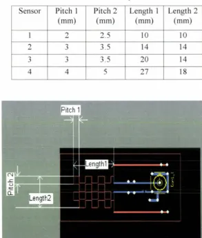
sensing coil [24]. The size of the sensor depends on the number of pitches used in that. The
optimum pitch size depends on the application [14].
•
Sensing coil Polyimide film (50 µm)Figure 2.2: Structure of the sensor
2.3 Design and Fabrication of Sensors
Three meander type and four mesh type sensors of varying lengths and pitches (table
2.1 and 2.2) were designed on Protel DXP 2004. The sensor schematics are shown in figure
Table 2.1: Meander sensor parameters
Sensor Pitch Length
(mm) (mm)
1 2 20
2 5 25
3 6 30
[image:27.574.180.371.95.219.2]4 8 40
Table 2.2: Mesh sensor parameters
Sensor Pitch 1 Pitch 2 Length 1 Length 2
(mm) (mm) (mm) (mm)
1 2 2.5 10 10
2 3 3.5 14 14
,.,
3 3.5 20 14
.)
4 4 5 27 18
Figure 2.3: Schematic diagram of mesh type sensor
[image:27.574.125.419.250.595.2]Figure 2.4: Schematic diagram of meander type sensor
It is seen from the diagrams that the coils are connected to a Bayonet Neill
Concelman (BNC) connector. The BNC connector is normally connected to a AC voltage
source through a coaxial cable. The AC voltage source drives the exciting coil. Since the
resistance of the coil is very low the sensing voltage is measured across a resistor of an
appropriate value. The two coils ( exciting and sensing) are designed on top of each other but
on opposite sides. On the schematics above the colour blue represents the exciting coil while
red represents the sensing coil. The exciting coil cannot be seen as the sensing coil overlaps
Figure 2.6: Fabricated mesh type sensors
2.4 Planar lnterdigital Sensors
The operating principle behind the interdigital sensor is very similar to the one observed in a parallel plate capacitor [29]. Figure 2. 7 shows the relationship between a parallel plate capacitor and an interdigital sensor, and how the transition occurs from the capacitor to a sensor. There is an electric field between the positive and negative electrodes and figure 2.7a, band c shows how these fields pass through the material under test (MUT).
Thus material dielectric properties as well as the electrode and material geometry affect the capacitance and the conductance between the two electrodes.
(a) (b) (c)
Figure 2.7: An interdigital sensor can be visualized as a parallel plate capacitor whose
electrodes open up to provide a one sided access to the MUT
The electrodes of an interdigital sensor are coplanar [29]. Hence, the measured
capacitance will have a very low signal-to-noise ratio. In order to get a strong signal the
electrode pattern can be repeated many times. This leads to a structure known as an
interdigital structure. The term "interdigital" refers to a digit-like or finger-like periodic
pattern of parallel in-plane electrodes, used to build up the capacitance associated with the
electric fields that penetrate into a material sample [29]. This is shown in figure 2.8 and the
side view shown in figure 2.9. In figure 2.8 one set of electrodes are connected or driven by
an AC voltage source while the other set are connected to ground. An electric field is
formed between the driven and the ground electrodes. This can be seen more clearly in
figure 2.9. It can be seen that the depth of penetration of the electric field lines vary for different wavelengths. The wavelength (A) of interdigital sensors is the distance between
two adjacent electrodes of the same type. In figure 2.9 there are three lengths ( /1, /2 and /3)
showing the different penetration depths with respect to the wavelength of the sensor.
Planar interdigitated array electrodes have many applications such as gas detection
[28], determining components in aqueous solutions [30], estimation of fiber, moisture and titanium dioxide in paper pulp [31, 32] and complex permittivity characterization of materials [27].
AC Voltage
Source
Gr
o
und
----
'
,,,.
'
l
.... .,,,-- - -
'
-
•
'
/
'
/'
···
'
..
.
.
..
··
··
..
\.
.
~ ~\
.. •
··
!
.
'\
Flexible
Electrode
Backplane
Figure 2.9: Electric field formed between driven and ground electrodes for different
wavelengths
2.5 Design and Fabrication of Interdigital Sensors
Four interdigital sensors of different wavelengths and lengths were designed on
Protel DXP 2004. The sensor parameters are shown in table 2.3 below. The sensor schematic is shown in figure 2.10.
Table 2.3: Interdigital sensor parameters
Sensor Wavelength, A Length
(mm) (mm)
1 5 20
2 6 30
,.,
8 40
.)
4 10 50
Figure 2.10: Schematic diagram of interdigital type sensor
The schematic diagram in figure 2.10 shows an interdigital sensor with 9 electrodes.
The BNC connector is connected to an AC voltage source, which in turn is connected to 4 electrodes as shown above. These four electrodes act as the excitation/driving electrodes.
The other five electrodes are connected to ground. When there is a material between the electrodes the electric fields from the driving electrodes penetrates through most of the material that is under test, and then terminates on the sensing electrodes. The electric field lines are affected by the dielectric properties of the material under test [27, 29, 31, 32]. Thus the potential or the current at the sensing electrodes is also a function of the material's dielectric properties. The advantage of using interdigital sensors is that it has on! y one sided access to the material under test [29]. Fabricated sensors are shown in figure 2.11.
2.6 Conclusion
Three different types of planar electromagnetic sensors are described in this chapter:
meander, mesh and interdigital configuration. The sensors are used for the estimation of
material properties in a non-invasive way, non-destructive way. The sensors generate a high
frequency electromagnetic field by carrying an alternating current. The generated
electromagnetic field interacts with the material under test and is modified. The modified
field is measured and is used for the estimation of system properties in an indirect way.
CHAPTER3
FINITE ELEMENT MODELING OF SENSORS
3.1
Introduction
In this chapter the characterization of all types of sensors, meander, mesh and
interdigital types have been carried out using finite element modeling. Before experimentation
all three sensors are modeled to analyze the distribution of electric field and magnetic flux. The
finite element software FEMLAB by COMSOL is used to model and analyze the field
distribution of all three types of sensors. FEMLAB solves all kinds of sci en ti fie and engineering
problems based on partial differential equations (PDEs).
Model Navigator
Space dimension: j3D
_j FEMLAB
I
I.::~ _j Electromagnetics Module
•-_:_i Statics • @i&MS#iiifflffi
t
•
Quasi-Statics, Small Currentst
.
Electromagnetic Waves•~ _J Acoustics
~ _:_i Diffusion
t
_J Electromagnetics±
_:_i Fluid Dynamics:e-
:J Heat Transfert
_:_i Structural Mechanics,+,-_J PDE Modes
Dependent variables: jV2 Ax2 Ay2 Az2 psi2
Application mode name: jqav2
.:.J
rMultiphysicsAdd Remove
_JGeom1 ~
L • ,,m&bJiftUDI
Dependent variables: V tAx tAy t ... Application Mode Propertie...
j
Add Geometry...
j
Ruling application mode: jauasi-Statics (qav)
Element: jA- Vector, V - Linear
.:.J
Multiphysics OK CancelApplication l\•tode Properties .~ ~
Properties- - - ~
Default element type: A-Vector, V - Linear
a
Analysis type: jTime-harmonic
Potentials: jElectric and magnetic Gauge fixing:
Ion
r
Apply changes to all application modesOK Cancel j
Figure 3 .1: FEMLAB model navigator
In the model navigator "Multiphysics" is chosen since electric and/or magnetic fields
are used to model the three types of sensors. Electromagnetics Module in 3-D mode is selected
and then Quasi-statics (qav) mode is chosen as shown in figure 3.1.
One of the effects of Maxwell's equation is that there is no synchronization between the
changes of the electromagnetic field and changes in time of currents and charges. Due to the
finite speed of propagation of electromagnetic waves the changes of the fields are always not in
line with respect to the changes of the sources. Quasi-static approximation involves ignoring
this effect, and obtaining electromagnetic fields by considering stationary currents at every
instant. The approximation can be considered valid given that the variations in time are small,
and that the models are considerably smaller than the wavelength.
Quasi-static analysis is used for the modeling of the three types of sensors. In
quasi-static analysis it is assumed that
aD
=
o
[3.1]at
Hence Maxwell's equations can be written as:
'vxH=J =a(E+vxB)+f
oB
'vxE=--'v•B=O
'v•D=p
'v•J=O ot
Table 3.1: Symbols used in the derivation
Symbol
H Magnetic field Strength
Je Externally applied current density
O' Electrical conductivity
E Electric field intensity
V Velocity of the conductor B Magnetic flux density
p Volume charge density
D Electric flux density
[3.2]
[3.3]
[3.4]
[3.5]
It is important that the currents and the electromagnetic field vary slowly in a quasi-static
approximation.
Using the definitions of the potentials,
B="vxA
aA
E=-'v'V--at
And the relationship between magnetic field, magnetic field strength and
Magnetization (M)
Ampere's law can be rewritten as
~ I ~
a - + 'y' X (µ; 'y' X A -M)- av X (V X A)+ dVV-;: Je,,
a,
[3.7]
[3.8]
[3.9]
[3.1 O]
Where A= magnetic vector potential and µ0 is the magnetic permeability of free space
Taking the divergence of the equation above gives the equation of continuity
aA
- "v.(a- - av x (V x A)+ dVV -P) = 0
at
[3 .11]In the "Application Mode Properties" dialog box the default element type is given as
A-Vector and V-Linear. Equations 3.10 and 3.11 give a system of equations for A and V.
A time harmonic analysis is chosen as the "Analysis Type" and both electric and magnetic
fields are chosen as the potentials. "Gauge Fixing" is turned on. Gauge transformation involves
a variable transformation of the potentials. The electric and magnetic fields are not uniquely
defined through the electric and magnetic potentials (equations 3.7 and 3.8).
Introducing two new potentials
A= A+ "v\f'
V
=
V -a\f'
a,
[3.12]
When substituted into equations 3.7 and 3.8 they give the same electric and magnetic fields,
E
= _
aA _vv
=
o(A -
V\J') _vcv
+al£')at at at
8A ~
- - - V V
ar
[3.13]~ ~
B
=
V X A= V X (A - V\J')=
V X A [3 .14]A particular gauge is chosen to obtain a unique solution. This means that constraints are
put on \J'. A constraint can also be put on V.A. If both V.A and V x A are given a vector field
can be uniquely defined up to a constant (Helmholtz's theorem). Coulomb gauge ( V.A =O) is
used.
The inductance (mesh and meander) and capacitance (interdigital) are calculated for a
range of frequencies. Hence Time-Harmonic Quasi-Statics is used. In 3-D time-harmonic
quasi-statics, both the electric and magnetic fields are used as the potentials. There is full coupling
between both the fields.
The equations are
- V.((jwo- - oi2&0)A - av x (V x A)+ (a-+ jw&0)VV -(P + jwP))
=
0 [3.15]where w 2 x n xf (frequency)
co is the angular frequency and/is the frequency
D = &0E
+
P is used for the electric field, where P is electric polarization3.2 Analysis of Planar Meander Sensor
The meander sensor has winding tracks [ 15, 17-19, 24] on the sensor substrate as shown
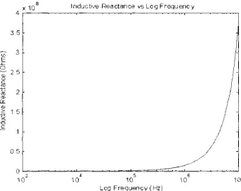
in figure 3.2. The aim of the modeling is to calculate the inductance of the meander coil for a
frequency range of 1 kHz to 10MHz, when placed in an environment. From the inductance the
inductive reactance can be calculated and the plotted against the frequency to see their
sl-StatlCCJ (qav): mecll'lder.fl ~. ~~
!:le !adt QptlOnS Qraw Phl'_,ics ~ :;ave ~ o cessrg ~ tjei,
-D c;;;; Iii sf;. ii, e Ji;" 6& ,t ~ = ~=-~1.iil J.,> ii if.I '11-i/Q .c'aon ©-O>! t
~~
·
1-i p
. ±
1/.!:!.
13
.
~,
v
·
.,.
I• ..
'@ s
~
Ii!
I!'!
k.
'OJ
(ii
l(-O!E33. -O.IE12. O.lll-l) S [GRio EQUAL CSYS
star,1 COMSO.., FEM.AB ... 1 !)FEM.doc.- - --· u,,,FEM.AII
-
=---Figure 3.2: Model of meander type sensor
The Reactance is calculated by
[3 .17]
where/is the frequency and Lis the inductance calculated from the model
:Memory: (156 . .t / 1£1U)
~~ 4:48PM
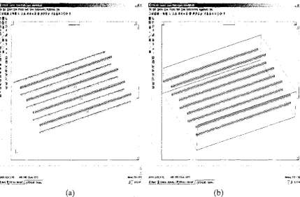
The meander sensor is modeled as shown above in figure 3.2. The large rectangular
block that surrounds the sensor acts as the environment the sensor is exposed to. The sensor is
initially modeled by individual blocks as shown in figure 3.3a. The individual blocks are then
connected together by creating a composite object of all the individual objects as shown in
figure 3.3b. The sensor block and the environment box are then made into one object as ·n
figure 3.4.
(aj ~)
Figure 3.3: Geometry of meander type sensor
In the "Boundary Settings" menu each boundary is defined according to the required
condition. The two sides of the sensor are provided an electric potential; one is assumed to be at
ground potential and the outer side is kept at a value of 1 V. All plates in the rectangular box
except the ones touching the sensor voltage and ground boundaries are set to "Electric
Insulation". All boundaries are set to "Magnetic Insulation" in the Magnetic Parameters menu.
The menu for setting the boundary conditions is shown in figure 3.4.
The electrical conductivity, relative permittivity and relative permeability are set in the
"Subdomain Settings" menu. The model has two subdomains: the sensor and the rectangular
box. Figure 3 .5 shows the window for setting the subdomain. There are two main regions,
copper and air. The frequency of operation can be set in the "Scalar Variables" dialog box.
,fie ~ ~ Q'- ~ ~ ~ toe!?'~ ~ ~
~
t
~•
.'-
- e,l_~_JD.A c ,e • Iii <a Jl>J:l,i,'.l,t-l 'l&ni.Jlaa n 0_~1 t flc-a P ,. [7 ~
a~
.
.
r_,,. ..
·
~
r11o1_..., ....
M..,.iicPn!MI..-. ~ • k P . - _ . . I
S.Clllc ~ ,_.,IN ""ttrltnl'
eo...i..., clOldeiofl jr:1tcrnc polN'II,.. ..:] o-...,. v•...t:•,,..._ ...
J.,
rciw,, I
v~ v,
i - - - -Rnr,nc,pa1W111t1 Eltctl'Cpoltmtl
~
'("1.S!Eih-~-0.135,0~l A.m {GACI feou•,1..ICSYs
fi:Jst.ar1l 1!,,1F94.e1oc-~.~Ul1FB'-9.AB-
OC!om-...,;;;;.451.,1u1
~ .. 9:
30»4-Figure 3.4: Window for boundary setting
E,le ~ Qpoons Q'"-Ph'pa ~ Sctw ~oonr,g ~ tleb
o"'i;i• , .. 111 •/..:.-6. 44 • ., ~ JOJ?Ji>'..-1-,1.,,1:,-,ogo, T
.
~fl
e-ll p ,.
,;, ~ •
.
.
ll>17
.
,.-•L-·
r:-
-
-l
= ~ . / ~-r,,•{9•"1•fcr•~\)'W-.fJ•O 6-o-•2;-.}'•V• lllo"\."1V• Al•nr•(V•~•(c,•,-fg\)'W•.f
l~a111 .. 11c1...
:::
1clC
::-.-::t~..::::;-
1
~
1
~
1
L.ilrwymM,nal.~ ~ r. ll•Mol'l,H r ••Mo"•
Qu,.... V"-IE•,...-r.1\(1,totiop,c) 1
C-8•._.,.H •B,
OncrlflN•
R .... ,..pe,m9Nilly
r I\ 1-.a1...,) rl ~. ,~,~, .~.~,- - - -Rtl•,.. ,. _ _.,
.
•. .,,--,---,----,...,,
-" • - - - . - -.... - - Vlllocily
.!SJ
~
!iie9,.,.-om.0CIM9) AlOSfGA!DfEotw.rCSYS
S<#t! l!!J-doc·---11.;fRM.AB--...
~ -,-S.9/74.l)
m~ .;;,,..
Figure 3.5: Window for subdomain setting
(-0.0435. -0.121, 0 058'2) AXIS' lGRlO ;eOUAL' fcsYs
/JttSt,rt! lilljFEMdo<: • MaosoL.11;1: COMSOL , FEM.AB .• jf;Ji FEM.AB • Geom ...
Figure 3.6: Mesh of the model
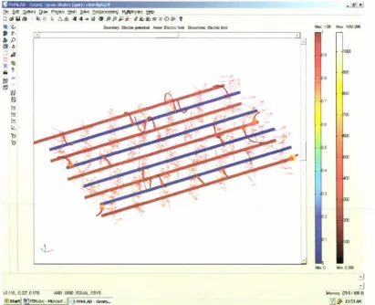
Figure 3.8 shows the solved meander sensor model for 500 kHz. The "tube streamlines" and the
arrows represent the magnetic flux density while the electric potential distribution is shown on
the surface of the sensor. While the electric potential ranges from O to 1 on the surface of the
sensor the magnetic flux density has a range from 4.026e-7 Tesla to 1.073e-4 Tesla.
tie !;iii: QplmS s!°"' l't-,,.cs !'!eS'1 ~
""'=ng
~""
t!OP Doi:" 5 it-, ~ .CS& at4=~ (JJ;)J;)jl,r •li2~aoooo, 1'• ~ ~ 8,ctric pottnrial ~<w. Magntdc tux den1~y StrHr'nin,: ~ ; e tux dtnsity
*
t-~ p ~~
"'
""~ ,;;;
'
@"'l!ll i!ll
~
::...
- --: ....
/ /
.. _;
-f-OOS-'5,-0.!B75,009AA} AXIS GAO EQUAL CSYS
CCM;Q., FBUll ... 111!!.]Fe.1.doc· Mio"ooof .•. 11,,FEH.AB-Geom •••
Figure 3.8: Solved meander model
Mu: 1.00 MIX: 1.073M
I xlo-'
.9
.8
.6
.5
.9
.8
.7
.6
.5
_,
.3
.2
.:J .:J Memory (154 7 / 100 ')
~~ 4:50PM
Once the solution is obtained different parameters can be calculated. For the meander sensor the
important paramete~ is the inductance. The inductance is calculated by
L = 2Wm
/ 2 [3.18]
where Wm is the magnetic energy stored, and I is the current flowing in the sensor.