Extraction and Recognition of Periodically Deforming Objects by Continuous, Spatio temporal Shape Description

Extraction and Recognition of Periodically Deforming Objects by Continuous,

Spatio-temporal Shape Description

S. D. Mowbray and M. S. Nixon

Electronics and Computer Science, University of Southampton,

Southampton, SO17 1BJ, UK

Abstract

We demonstrate a novel approach to modelling arbi-trary temporally-deforming objects using spatio-temporal Fourier descriptors. This is a continuous boundary descrip-tor, which can handle shapes that vary in a periodic man-ner (such as a walking subject). As such, we can handle non-rigid, moving shapes that self-occlude. We show how this approach has led to successful shape extraction and de-scription with both laboratory-sourced and real-world data. A consequence of exploiting temporal shape correlation in this approach has led to very good tolerance of noise and other positive performance factors. Further to this, our new approach holds sufficient descriptive power not only for ex-traction, but also for description purposes, and we have been pleased to note high recognition rates in human gait recognition on a large database.

1. Introduction

1.1

Finding Periodically-Deforming Objects

A prerequisite to being able to use an object’s shape as means of recognizing it is the ability to successfully detect the particular shapes of interest in an image sequence. This is not a trivial problem and one which has been studied in the past by means of utilizing various forms of the Hough transform. In particular, there are two spatio-temporal ver-sions of the Hough transform that extract shapes that move through time [13, 7]. Evidence-gathering techniques, such as these,votefor free parameters of the shape model, typ-ically the shape’s location in a Cartesian space, although other parameters such as scale and orientation may also be sought.

Previous approaches to finding moving shapes have only dealt with static shapes, whereas many shapes in the real-world, especially the shapes of live subjects, deform in a periodic manner as they move. Through the use of spatio-temporal Fourier descriptors, a new variant of the Hough transform is developed, which can extract moving,

de-formable objects from an image sequence (such as walking human subjects). This new evidence-gathering technique not only proves to inherit many desirable features from the standard Hough transform, such as its ability to deal with noise and occlusion, but also provides a continuous, spatio-temporal shape representation to deal with the effects of dis-cretisation, and the computational benefit of having a pa-rameter space with a fixed number of dimensions, whilst still being capable of describing arbitrary shapes, shape de-formation, and motion.

1.2

Gait as a Biometric

Recently, a significant amount of attention has been devoted to the use of human gait patterns as a biometric and to the analysis of human motion in general. Several models have been proposed for the description of the human body and also for the description of human gait [1, 6]. Human gait has many advantages over other biometrics, but perhaps its two most notable advantages are that it is non-invasive – of-fering a means to verify identity without a subject’s active participation, and that it offers a means of offering recogni-tion at a distance.

This study demonstrates a new, model-based approach that captures the full movement and deformation of the body, rather than just a specific body part, and by utilizing only the boundary information of the object.

2

Spatio-Temporal Fourier

Descrip-tors

Two-dimensional shapes are usually represented on a Carte-sian plane, where thexandyco-ordinates of the shape can be thought of as a function of the shape’s arc-length index,

l. If we define a mapping from the Cartesian plane to a complex plane, however, then we can represent a shape’s boundary as a complex function of arc-length:

c(l) =x(l) +j.y(l) (1)

Due to the periodicity ofc(l)it is possible to represent the shape’s boundary using a Fourier series, with the coeffi-cients of the series,axk,bxk,ayk, andbyk, being the Fourier

descriptors of the shape:

c(l) = ax0

2 +

∞

k=1

axkcoskl_L2π+bxksinkl_L2πdk+

j

ay0

2 +

∞

k=1

aykcoskl_L2π+byksinkl_L2πdk

(2) If we now consider a shape which deforms betweentand

T in time, we can model the periodicity of the deforming shapes, at arc-length indexlas

s(t, l) =s(t+T, l) (3)

Given this, it is possible to model the whole periodically deforming boundary of a shape in this shape sequence as a two-dimensional complex Fourier series:

s(t, l) = ∞

kt=0

∞

kl=0

ˆ

s(kt, kl)ej2π

t.kt

T +l.klL

dkldkt (4)

given here in complex form for brevity. The Fourier co-efficients of this series characterize one whole period of the shape’s movement.

If we consider the discrete case for a periodically de-forming and moving shape thenTis equivalent to the num-ber of images in one period of motion, L represents the length of the boundary of the object, indexed byl, and the Fourier coefficients, ˆs, can be calculated using a discrete, two-dimensional, complex Fourier transform.

ˆ

s(kt, kl) = 1

T.L

T

t=0

L

l=0

s(t, l)e−j2π

kt.t T +kl.lL

(5)

We have earlier investigated the descriptive properties of spatio-temporal Fourier descriptors [12] and now show that we can also use them as a basis to formulate a new extrac-tion technique with the capability of extracting periodically-deforming shapes from real-world imagery.

3. The Continuous Deformable Hough

Transform

3.1

Background

Many image sequences contain a significant amount of tem-poral correlation, a fact which is frequently utilized by video compression techniques. The Velocity Hough Trans-form (VHT)[13] was the first evidence-gathering technique to use this correlation to extract the optimal parameters of a linearly moving conic section. Simple extensions to the VHT made it possible to extract any shape and motion com-bination, given that both were able to be modelled paramet-rically.

The VHT was originally developed as an extension of the Hough Transform for circles by adding a velocity parameter into the formulae used to cast votes into the accumulator space. The original VHT extended the Hough transform for circles to include velocity, as follows:

ax=cx+r.cos(θ) +vx.t

ay =cy+r.sin(θ) +vy.t (6)

where ax anday are the coordinates of the vote to be

cast,cxandcyare the center coordinates of the circle to be cast into the accumulator,randθare the polar parameters of the circle in question,vxandvy describe the linear ve-locity of the circle andtrepresents a time reference relative to the start of the object’s motion.

During the voting process, the time reference,t, and the x-axis and y-axis velocities,vxandvy, are used to deter-mine the location of the center coordinates of the circle in the initial frame of motion, att= 0, therefore focusing all votes for the correct circle onto one set ofaxanday

coordi-nates. Thus, the coordinates voted for when using the VHT are the center coordinates(ax, ay)of the circle at its initial

time reference with a linear velocity described by(vx, vy).

The VHT was extended[7] to include a continuous shape model, using Elliptic Fourier Descriptors, to create the Con-tinuous Velocity Hough Transform (CVHT). Using a con-tinuous shape model ensures that discretisation errors, usu-ally associated with applying affine transformations to dis-cretized shape models, can be minimized, and also allows for undetermined points in a shape model to be interpolated with ease.

Deformable Hough Transform, which is specifically de-signed to deal with non-rigid, moving shapes.

3.2

Theory of The Continuous Deformable

Hough Transform

If we represent a spatio-temporal shape sequence, as de-scribed in section 2, as a complex Fourier descriptor matrix,

ˆ

s(kt, kl), then we can define a kernel that defines the shape of votes to be cast in the accumulator space for each feature point in a test image sequence (each edge pixel). This ker-nel is a combination of shape sequences, at various spatial, temporal, and motion scales.

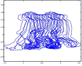
The basis for the CDHT kernel is a normalized shape se-quence descriptor, derived from Eq. 5. This is the complex spatio-temporal Fourier descriptor matrix of the shape we wish to find in the test sequence. The shape sequence de-scriptor is normalized so that the shape’s maximum height and width with respect to the whole image sequence are set to unity. One drawback to this normalization approach is that the aspect ratio of the shape is lost. There are rea-sons for this, however, particularly when the technique is applied to finding humans, as humans themselves do not have a fixed aspect ratio, and thus allowing non-uniform scaling of both width and height (and therefore justifying normalization of both) is applicable here.

The motion model, provided by the spatial DC compo-nents, is also normalized independently of shape size so that the linear distance that the shape travels (in its direction of motion) falls in the range[0,1), with the shape’s initial cen-ter of mass at the beginning of the shape sequence being

(0,0). An example of a reconstructed normalized shape se-quence descriptor is shown in Figure 1.

−1.5 −1 −0.5 0 0.5

−0.6 −0.4 −0.2 0 0.2 0.4 0.6 0.8

Figure 1: Example normalized shape sequence descriptor

During the following formal definition of the kernel of the CDHT, the normalized shape sequence descriptor ma-trix, as described above, will be referred to as the Shape Se-quence Template (SST). This is simply a matrix of spatio-temporal descriptors from which the algorithm can recon-struct a normalized trace of a shape sequence.

The CDHT kernel,ω¯, can thus be defined as being the rescaled version of aSST, for all scale values we wish to search for, transformed into the time domain:

¯

ω(t, l, xs, ys, ts, vs) = KT−1

kt=0

KL−1

kl=0

SST(_{kt, kl, xs, ys, ts, vs})e j2πkll

KL _dkl e j2πktt

KT _dkt

(7) where SST(kt, kl, xs, ys, ts, vs) is a scaling function

which scales the SST appropriately for the spatial scaling variables, xs andys, the temporal length of the sequence

(in frames),ts, and the ‘velocity’ scale factor,vs. The

sep-arate velocity scaling factor is required here, as we should not assume a relationship between shape-size and velocity, or sequence-length and velocity.

3.3

The CDHT Voting Process

The kernel defines the shape sequence of votes to be cast into the accumulator for each feature point (edge pixel) in a test image sequence. This is a combination of shape se-quences at varying spatial, temporal, and velocity scales.

Each sequence of votes is cast into the accumulator by offsetting it from the co-ordinates of each feature point in the test image sequence,IS, defined by

IS=λ¯(f,p)|f ∈Df, p∈Dp (8)

where λ¯(f,p) is a function that defines the feature points,pwith co-ordinates(px, py), in an image for each frame,f, in an image sequence, andDpandDfdefine the domains of pixels in an image and frames in an image se-quence respectively.

Given this, the accumulator vote function is defined as

Afp=

_¯

λ(f, px)− {ω¯(f−t, l, xs, ys, ts, vs)},

¯

λ(f, py)− {ω¯(f−t, l, xs, ys, ts, vs)}

(9) wheret∈Dt, l∈Dl, f ∈Df,p∈Dpforf ≥twhere

Dtis the domain of the possible temporal locations for the

start of the shape sequence andDlis the domain of the

arc-length parameter of each shape. Afpthen defines a set of

vote coordinates for which votes will be cast in the accumu-lator. It is necessary to decompose the kernel here into its real and imaginary parts, which determine the offsets along the x-axis and y-axis respectively of the feature point from the location of the vote in the accumulator.

With the accumulator vote function now defined, it is now necessary to define a matching function that will map the vote coordinates in setAfpinto the accumulator space.

simply increments a matched accumulator point by unity:

M(α,a) =

1 α=a

0 α=a (10)

This matching function is then applied toAfpfor a range

of parameter values, thus fully defining the continuous ver-sion of the CDHT as

CDHT(δ, t, xs, ys, ts, vs)=

l F t=0

F f=t

p

M(δ, t),λ¯(f,p)−ωdp df dt dl (11)

where

ω≡

{ω¯(f−t, l, xs, ys, ts, vs)}, {ω¯(f−t, l, xs, ys, ts, vs)}

(12)

In Eq. 11,δis the spatial translation vector andtis the temporal translation (in frames) to the center of mass of the first shape in the shape sequence. This continuous param-eter space is then sampled into a discrete paramparam-eter space, given by

DCDHT(δ, t, xs, ys, ts, vs)=

l∈Dl F t=0

F f=t

p∈Dp

M(δ, t),λ¯(f,p)−ω (13)

with the global maximum of this space being indexed by the estimated parameters of the shape-sequence model appearing in the image sequence.

3.4

Noise Analysis

The Hough transform and its derivatives are well known to be very robust to noise due to their implicit evidence-gathering properties. Noise tends to lead to false feature points in the image sequence, and as such, false loci of votes in the accumulator of the Hough transform. Conversely, however, any true feature points (edge pixels of the actual shape sequence) remaining after the addition of noise will also cast loci of votes in the accumulator, which should co-incide to provide a global maximum indexed by the correct parameters of the shape. So long as the global maximum of the accumulator is large enough to not be masked by the noise then the correct shape sequence parameters will be found.

The image sequence used in the noise performance tests was derived from the Fourier descriptor-based shape se-quence template of a real-world image sese-quence. Using this shape sequence template the test sequence was recon-structed at a low resolution in order to make the computa-tional demands of the performance tests detailed here feasi-ble. Although the test image sequence is not a true synthetic image sequence, as it is generated from imagery of the real-world, it can be considered to be synthetic as there is no

background noise, with the only feature pixels being from the shape sequence itself. Edge detection is obviously not necessary (and perhaps not desirable) on a synthetic image sequence such as this, as all we wish to compare is the effect of noise, rather than the performance of an edge detector at removing noise and detecting true edges. All real-world image sequences would obviously need to be edge detected prior to being used as input to the CDHT.

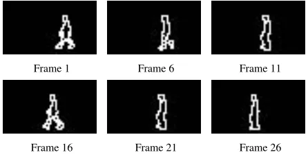
Selected frames from the test image sequence are shown in Figure 2

Frame 1 Frame 6 Frame 11

Frame 16 Frame 21 Frame 26

Figure 2: Synthetic Shape Sequence

The CDHT was tested for its robustness to noise using 11 noise levels, from 0% – 100%. An effective and ade-quate noise model for binary synthetic edge data (such as that used here) is to simply add false edge pixels to the background and false background pixels to true edges with equal probability (where a background pixel is assumed to be 0 and an edge pixel a 1), in effect, a form of salt and pepper noise. If we presume no previous knowledge of the image then we can assume each pixel has an equal prob-ability of being a background pixel or an edge pixel and therefore to add noise we can merely assign a pixel in the image to be either a background pixel or an edge pixel, with equal probability. For example, adding 10% noise would change roughly 5% of the background pixels into edge els and roughly 5% of the edge pixels into background pix-els. At 100% noise, the image would contain a purely ran-dom distribution of edge and background pixels, with any true background or edge pixels remaining only by chance. The varying noise levels used during testing, added to one frame from the test sequence, are shown in Figure 3.

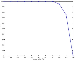
The result of the noise performance test using a set of fifty noisy sequences corrupted by varying levels of random noise is shown in Figure 4.

10% noise 20% noise 30% noise 40% noise 50% noise

60% noise 70% noise 80% noise 90% noise 100% noise

Figure 3: Frame 16 with varying noise levels added

0 10 20 30 40 50 60 70 80 90 100 0

10 20 30 40 50 60 70 80 90 100

Image noise (%)

Hit rate (%)

Figure 4: Noise performance

both spatially and temporally at noise levels of up to 80%. The ability to tolerate such extreme levels of noise is due to the global spatio-temporal evidence gathering nature of the CDHT. For example, if one frame in the CDHT is cor-rupted to a point where it is no longer recognizable, then this does not have such a great impact on the final result, whereas other evidence gathering techniques, such as the GHT are limited to the amount of information contained in one frame of an image sequence, which may prove to be in-sufficient to track the object correctly if the object becomes occluded.

3.5

Real-world image data

The above results indicate that the CDHT works well when given a synthetic input, but in practice edge detected im-ages sequences are never so well defined. Noise is usually always present in an image to some extent, and even the best edge detection techniques result in false edges being de-tected while true edges are not. Due to this, the CDHT was tested on the real-world image sequence, selected frames of which are shown in Figure 5.

The image sequence shown in Figure 5 was first edge de-tected using the Canny operator [3] to create a binary edge image, the input of which was fed directly into the CDHT. The Shape Sequence Template used to form the basis for the

Frame 1 Frame 7 Frame 13

Frame 19 Frame 25 Frame 31

Figure 5: Example real-world image sequence

CDHT was the same as that used during the synthetic noise performance tests, except that the direction of motion was left-to-right, rather than right-to-left – a transformation re-quiring only a simple flipping of the Shape Sequence Tem-plate and a sign inversion of the DC component. The re-sults of this test is shown in Figure 6, with the reconstructed Shape Sequence Template, scaled and offset by the param-eters found using the CDHT, overlaid on top of the original image sequence.

Frame 1 Frame 7 Frame 13

Frame 19 Frame 25 Frame 31

Figure 6: Results of the real-world data test

4

Human Gait Recognition

Access to the spatio-temporal frequency domain of the shape sequence provides a convenient method of analyz-ing fundamental structural properties of the shape sequence, and as such the spatio-temporal Fourier descriptors provide a good theoretical basis for discriminating between shape-sequences and therefore for classification and recognition of deformable objects.

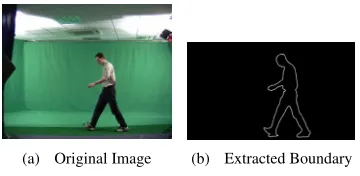
To test the recognition capabilities of this technique, spatio-temporal Fourier descriptors were calculated for each subject in the Large Gait Database at the University of Southampton [14]. This database consists of 115 subjects and 1062 sequences (only right-to-left walking sequences were used for this test). In order to extract the boundary for each shape in an image sequence background extrac-tion is first performed on each image (via chroma-keying), then each image is thresholded to produce a silhouette. The boundaries from each subject are then extracted by follow-ing the outer contour of each image, startfollow-ing from the top of the head, to produce a complex boundary signal (see Figure 7), from which the spatio-temporal Fourier descriptors are calculated.

(a) Original Image (b) Extracted Boundary

Figure 7: Boundary Extraction

The descriptors produced using the method described above contain a large number of elements. In order to use these descriptors for classification purposes it is necessary to reduce the number of descriptors for each subject. This is necessary for two reasons, firstly to extract only the descrip-tors that would be useful for classification, and secondly to reduce the dimensionality of the feature space, thus ensur-ing feasible classification speeds.

The primary aim of feature selection in this case is to minimize intra-subject variance and maximize inter-subject variance, in order to increase the Correct Classification Rate (CCR). To achieve this one can use a variation of the Bhat-tacharyya distance metric to measure inter-class separation due to mean-difference with respect to the class covariances [5]. The separation between the two classesaandb, for a given feature, is given by

Sa,b = [ma−mb]

a+

b

2

−1

[ma−mb]T (14)

wheremais the class mean and_ais the covariance matrix of classa, with equivalent terms for classb.

To gain a measure of a feature’s ability to separate classes successfully a mean value ofSwas determined for each feature as

¯ S= 1

D2

D

a=1

D

b=1

Sa,b (15)

whereD is the number of descriptors available. S¯is then proportional to the class separability measure of the given feature, with larger values ofS¯implying good class separa-bility.

Classification testing used twenty features selected us-ing the method described above as havus-ing the highest class separability values.

Classification was performed using a K-nearest neigh-bour classifier and cross-validated with the leave-one-out rule. This classifier assigns a test subject to be the same class as that of the modal class of thekthnearest neighbour-ing subjects to it. If no modal class is found, then the test subject is assigned to the class of the nearest neighbouring subject. The distance between classes is measured by the Euclidean distance,ED, given by

ED= N−1

n=0

(xn−yn)2 (16)

whereNis the dimensionality of the feature set, andxnand

ynare the values of thenthfeature of the samplesxandy respectively.

The classification results fork= 1andk= 3are shown in Table 1.

Table 1: Results of k-nearest neighbour classification

Database k CCR(%) SOTON 1 84.5 SOTON 3 86.2

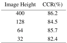
The performance and robustness of using Fourier de-scriptors for the recognition of deformable objects was eval-uated at varying resolutions, to simulate the effects of dis-tance. As mentioned in Section 1.2, human gait as a bio-metric has the unique advantage of being useful at vary-ing distances. To test the performance of spatio-temporal Fourier descriptors the effects of distance are simulated and performance testing is performed. The effect of distance is simulated by decreasing the spatial resolution of each image in an image sequence. The original images, which were at a resolution of 690 x 400, were scaled so that their heights were 128, 64, and 32 respectively. The results of classifi-cation at these resolutions, shown in Table 2, show that the image resolution can be relatively small without a great loss of resolution.

The fact that such a loss of spatial resolution results in only a small drop in recognition rate can be accounted for by the facts that the majority of the information in a given Fourier descriptor is contained in the low-level descriptors and that for a spatial boundary of lengthN we can obtain up toN₂ descriptors. Therefore, as long as we have a suffi-ciently large value ofN, an adequate number of descriptors can be obtained for recognition. This requirement is more than fulfilled, even at the low resolutions used here.

Table 2: Results of k-nearest neighbour classification (k=3) for varying resolutions

Image Height CCR(%) 400 86.2 128 84.5 64 85.7 32 82.4

5

Conclusions

The aim of this research was two-fold. In the first instance, the aim was to combine the powerful descriptive power of spatio-temporal Fourier descriptors with the robustness of the Hough transform, resulting in a new algorithm for the detection and extraction of deformable moving objects. The second aim was to test the capability of spatio-temporal Fourier descriptors to describe deforming moving shapes and to test their discriminatory power, in this case by ap-plying them to the field of automatic gait recognition. In summary, spatio-temporal descriptors provide a new multi-scale approach to describing temporally deforming shapes with the power to describe shape and deformation in a gen-eralized way, suitable for shape extraction, and also in a more detailed way, suitable for shape discrimination.

Acknowledgments

We gratefully acknowledge partial support by the Euro-pean Research Office of the US Army under Contract No. N68171-01-C-9002.

References

[1] J. K. Aggarwal and Q. Cai. Human Motion Analysis: A Review.CVIU, 73(3):428–440, March 1999.

[2] C. BenAbdelkader, R. Cutler, and L. Davis. Motion-based recognition of people in eigengait space. InProc. 5th FGR 2002, pages 254–259, 2002.

[3] J. Canny. A Computational Approach to Edge Detection.

IEEE Trans. PAMI, 8(6):679–698, 1996.

[4] J.P. Foster, M.S. Nixon, and A. Prugel-Bennett. Automatic gait recognition using area-based metrics. Pattern Recogni-tion Letters, 24(14):2489–2497, October 2003.

[5] K. Fukunaga.Introduction to Statistical Pattern Recognition. Morgan Kaufmann, 2 edition, 1990.

[6] D. M. Gavrila. The Visual Analysis of Human Movement: A Survey.CVIU, 73(1):82–98, January 1999.

[7] M.G. Grant, M.S. Nixon, and P.H. Lewis. Extracting mov-ing shapes by evidence gathermov-ing. Pattern Recognition, 35(5):1099–1114, May 2002.

[8] J.B. Hayfron-Acquah, M.S. Nixon, and J.N. Carter. Auto-matic gait recognition by symmetry analysis.Pattern Recog-nition Letters, 24(13):2175–2183, September 2003.

[9] P. S. Huang, C. J. Harris, and M. S. Nixon. Recognising humans by gait via parametric canonical space. Journal of Artificial Intelligence in Engineering, 13(4):359–366, 1999.

[10] A. Johnson and A. Bobick. A multi-view method for gait recognition using static body parameters. In Proc. 3rd AVBPA 2001, pages 301–311, June 2001.

[11] A. Kale, A. N. Rajagopalan, N. Cuntoor, and V. Kruger. Gait-based recognition of humans using continuous hmms. In

FGR02, pages 321–326, 2002.

[12] S. D. Mowbray and M. S. Nixon. Automatic Gait Recogni-tion via Fourier Descriptors of Deformable Objects. InProc. 4th AVBPA 2003, pages 566–573, 2003.

[13] J. M. Nash, J. N. Carter, and M. S. Nixon. Extracting moving articulated objects by evidence gathering. InProc. BMVC98, volume 2, pages 609–618, 1998.

[14] J. D. Shutler, M. G. Grant, M. S. Nixon, and J. N. Carter. On a large sequence-based human gait database.Proc. RASC02, pages 66–71, 2002.