Selecting and fitting graphical chain models to longitudinal data

Selecting and fitting graphical chain models to longitudinal data

Riccardo Borgoni, Ann M. Berrington and Peter W. F. Smith

Abstract

The aim of this paper is to demonstrate how graphical chain models can be used as effective tools in life course research focusing in particular on models for longitudinal prospective data. The substantive research question focuses on whether young motherhood is a pathway through which socio-economic disadvantage in childhood is related to poor self-reported health in adulthood among the 1970 British birth cohort. By breaking down large multivariate systems into simpler more tractable subcomponents and analysing them via local regressions, graphical models helps the understanding of complicated life course processes, show the intermediate relationships between predictors, and aid the understanding of the mechanisms through which potential confounding and mediating factors affect the outcome of interest.

Selecting and fitting graphical chain models to longitudinal data

Riccardo Borgoni, Ann M. Berrington and Peter W. F. Smith

Social Statistics Division and Southampton Statistical Sciences Research Institute

University of Southampton

Addresss for contact:

Riccardo Borgoni

Social Statistics

University of Southampton

Southampton

UK

SO17 1BJ

Tel: +44 (0)2380 595673

Fax: +44 (0)2380 593846

Email:

[email protected]

Date: March 2004

Abstract:

The aim of this paper is to demonstrate how graphical chain models can be used as effective tools in life course research focusing in particular on models for longitudinal prospective data. The substantive research question focuses on whether young motherhood is a pathway through which socio-economic disadvantage in childhood is related to poor self-reported health in adulthood among the 1970 British birth cohort. By

breaking down large multivariate systems into simpler more tractable subcomponents and analysing them via local regressions, graphical models helps the understanding of complicated life course processes, show the intermediate relationships between predictors, and aid the understanding of the mechanisms through which potential confounding and mediating factors affect the outcome of interest.

Keywords

: graphical modelling, path analysis, life course, health inequalities, attrition weights

Acknowledgements:

1. Introduction

Graphical models and chain graph models are powerful tools to investigate complex systems consisting of a large number of variables (Wermuth and Lauritzen, 1990). In spite of this there are few examples of their application in the literature. Notable exceptions are, for example, Mohamed et al. (1998), Magadi et al. (2002), Cheung and Anderson (2003). The aim of this paper is to demonstrate how graphical models can be used as effective tools in life course research focusing in particular on models for longitudinal prospective data. Graphical chain models are ideally suited to situations where we have prospective data collected in sweeps of a longitudinal survey. The temporal ordering of the data helps identifying the causal ordering of variables across the life course. Graphical models can investigate the complex pathways through which earlier life course experience are related to later experiences. Graphical chain modelling can help cope with attrition as the available sample can be use in each stage of the chain confining the potentially serious effect of drop-out to the late components of the chain. In contrast to structural equation models, graphical models are better able to handle categorical data - the type of data often collected within social science surveys. Depending upon the precise outcomes being modelled (binary, categorical, single outcome, multiple

outcome), we can use the most appropriate regression tool, be that a binary or multinomial logistic model, or a loglinear model where multiple outcomes are simultaneously modelled. There are some issues relating to the practicality of fitting graphical models, including the fact that, depending on model search criteria, they can be computationally expensive, and when considering high dimensional processes we can run into problems due to data sparseness. Here we suggest practical solutions to these problems using an example from a study investigating teenage motherhood as a pathway through which socio-economic disadvantage in childhood is related to poor self-reported health in adulthood.

2. Back ground of the study and the data

Our example comes from a research project investigating whether young motherhood acts as a mediating pathway through which social disadvantage in childhood is associated with poorer health in early adulthood. Using prospective data and graphical modelling we examine the pathways associated with becoming a young mother and the pathways between young motherhood and poor health in adulthood. In the following sections we describe the conceptual framework, and the data used in the analysis.

2.1 Conceptual Framework

This paper takes a life course approach viewing an individual’s experience as an outcome of their changing development and changing context (Elder, 1985). Young motherhood is seen as the result of a complex series of individual, family and societal factors. Consequences of early parenthood depend on these factors and on mediating factors following the birth, which may include living arrangements, financial

Figure 1: Conceptual Framework

Block 1:

Parental background

Birth order

Block 3:

Age at motherhood

Mother’s

age

first

birth

Region

of

birth Block

4:

Block

6:

Partnership

Health at

Ethnicity

Dissolution

age 30

Father’s

social

class

Block 2:

Parental

education

Childhood characteristics

Receipt of benefits

Social

housing

.

Ever in care

Family structure

Reading

ability

Locus

of

control

Parental aspirations for age

will

leave

school

Anti-social behaviour

Block 5:Current circumstances

Non-working household

Social network

Household composition

Social housing

Closeness to mother

Satisfaction with area

2.2 The 1970 British Birth Cohort Study

The study sample are a nationally representative sample of women born in Britain in 1970 who have been followed up from birth within the 1970 British Cohort Study (BCS70). See Ferri et al. 2003 for further details of the survey. In total the cohort has been surveyed at birth, age 5, 10, 16, 26 and most recently at age 301. In this paper we confine ourselves to using data from the birth, age 10 and age 30 sweeps. In this way we minimize missing data and loss from the survey, whilst keeping important information about parental background and childhood experiences of the cohort member. As for any longitudinal study there has been attrition from the sample. Of 7392 females born in Britain and who took part in the birth survey, 64% took part at age 30. For each block of the analysis we use all the available cases. Attrition weights are used to compensate for the disproportionate loss-to follow up of more disadvantaged subjects (Little and Rubin, 2002). See Appendix 1 for details of how the weights are estimated. Any remaining item non-response is dealt with by imputation. We first look to see whether the missing information is available in another sweep of the survey. If not, we use a hot deck procedure for which the donors are identified through the terminal nodes of a classification tree. (See Borgoni and Berrington, 2004 for a description of the multivariate imputation procedure.)

2.3 Outcome Variable – self reported general health

At age 302 subjects are asked “how would you describe your health generally?” Response categories were “excellent”, “good”, “fair” or “poor”. We use a binary outcome comparing those who report their health as “excellent” or “good”, with those who report their health has being either “fair” or “poor”. In our sample 15.2% (weighted estimate) of women report less than good health. This estimate is very similar to that obtained for women aged 25-34 in the 1998 English Health Survey (14%) (Office for National Statistics, 2000).

1

Wave non-response at the age 16 survey, which was conducted through schools, was particularly high due to a national teacher’s strike. The age 26 survey consisted of a short postal questionnaire and was also affected by high non-response.

2

2.4 Explanatory variables

Explanatory variables are chosen on the basis that they have previously been shown in the literature to be either associated with age at motherhood (Kiernan and Hobcraft, 1999; Maughan and Lindelow, 1997; Jafee, 2002; Cheesbrough, 2003), or with the development of social inequalities in health over the life course (Power and Manor, 1992; Power et al., 2002; Sacker et al., 2002).

Block 1 contains parental background and birth characteristics and includes whether the cohort member was a first or higher order birth, their own mother’s age at first birth (aged under 20, aged 20-24, 25 and above years), father’s occupational social class (professional and intermediate, junior non-manual, skilled manual, semi and unskilled, and no father figure), parental education (with those whose only parent (in the case of lone parents), or both parents (in two parent families) left school at or before age 16 being identified separately. Due to the small number of respondent’s in individual minority ethnic groups the respondent’s ethnicity is categorized into two broad groups: White or non-White.

each statement range from “does not apply” (score of 0) to “certainly applies” (score of 100). Reliability was high (Cronbach’s alpha was 0.80). The total score is the sum of the score on each of the items and those falling in the top 10% are identified as exhibiting behavioural problems.

Age at motherhood is entered as Block 3 (under 20 years, 20-23 years, 24-30 years, and not yet a parent). Block 4 identifies whether the respondent has experienced partnership dissolution. Block 5 contains adult circumstances including whether the respondent lives in family with no adult worker, whether they live in social housing, whether they are the lone adult in a household, whether they are satisfied with the area in which they live, whether they are (emotionally) close to their mother, and whether they have a supportive friend in whom they can fully confide.

3. Graphical modelling

A graphical model is a stochastic model specified via a mathematical graph. Recent monographs on this subject include Whittaker (1990), Cox and Wermuth (1996), Lauritzen (1996), Cowell et al. (1999), Edwards (2000) and Pearl (2000). Below we review some key ideas and the terminology of graph theory and

graphical modelling.

3.1 Graph Theory

A graph is a pair of sets G=(V,E) where V is a finite set of nodes (vertices) and E is a set of edges. Two nodes connected by an edge are called adjacent. The edge can be directed, also called an arrow, or

undirected. The edge connecting two nodes α and β is a direct edge pointing to β if (α, β) ∈ E but (β,α) ∉ E. If (α, β)∈E and (β,α)∈E then there is an undirected edge between α and β. A path is a sequence of adjacent

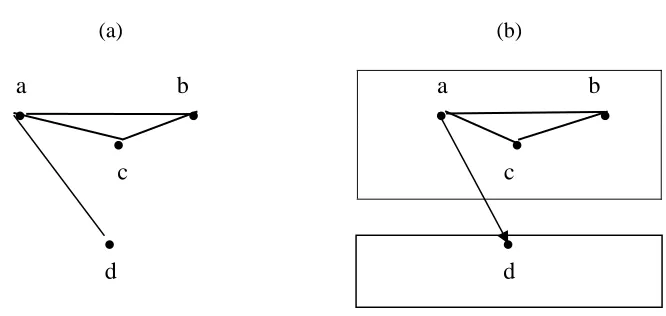
nodes. A graph is acyclic if it does not contain any directed cycle, a directed cycle being defined as a path from a node back to itself following a directed route (a direction preserving path). Figure 2a shows an acyclic graph G for which V={a, b, c, d} and E={(a,b), (b,a), (a,c), (c,a), (a,d), (d,a), (b,c), (c,b)}. The sequence of nodes a, b, c identifies one possible path from a to c. Removing (c,a) from E replaces the undirected edge between a and c with an arrow from a to c. This makes the graph cyclic as now the direction preserving path

A clique in a graph is a subset of nodes which induce a complete subgraph (i.e. a subgraph all of whose nodes are directly connected by an edge or an arrow) such that the addition of a further node makes the graph incomplete. The subgraph identified by the set of nodes {a, b, c} in Figure 2a, for instance, is a clique of the graph.

Figure 2: (a) An acyclic graph (b) A chain graph

(a) (b)

a

•

b

•

a

•

b

•

•

c

•

c

•

d

•

d

A chain graph is obtaining by partitioning the set of nodes in subsets called blocks or components. Nodes in different blocks are always joined by arrows while any edge is undirected for intra-block nodes. This component formulation excludes graphs with cycles. Nodes belonging to the same component are usually gathered into a box. Figure 2b shows a simple 2-block chain graph. A chain graph for which each component is a singleton is called a Direct Acyclic Graph (DAG). However, a chain graph may be more general than a DAG as here a mixture of directed and undirected edges is permitted.

3.2 Graphical models

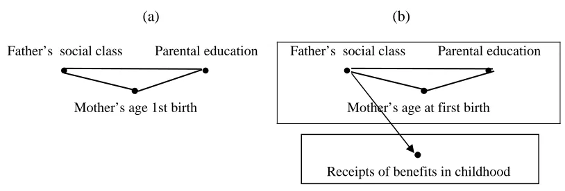
Here nodes represent random variables3 and undirected edges (lines) the interaction between pairs of variables. Asymmetric relationships between variables, i.e. one anticipates in some sense the other, are represented through arrows. Figure 3a depicts a hypothetical graphical model, including three variables considered later on in the paper, containing interactions between pairs of variables, namely father’s social class and parental education, father’s social class and mother’s age at first birth and finally mother’s age at first birth and parental education.

3

Figure 3: (a) a graphical model and (b) a chain graph

(a) (b)

Father’s social class

•

•

•

•

•

Mother’s age 1st birth

•

Mother’s age at first birth

•

Receipts of benefits in childhood

Figure 3b displays a two component chain graph model. A partial direction preserving path in a chain allows the representation of both direct and indirect effects. In Figure 3b for instance it is possible to identify a direct effect of father’s social class on the receipt of benefits in childhood, as well as an indirect effect of parental education on the receipt of benefits through father’s social class.

Fundamental to graphical modelling is the concept of conditional independence. Let X=(Xα, α∈V) be a collection of random variables regular enough to ensure the existence of conditional probabilities. A graphical model uses a graph with nodes in V to specify a set of conditional independence relationships amongst the elements of X. These relationships are called Markov properties and a graphical model is

sometimes called a Markov graphical model. In particular, in an undirected (conditional) independence graph an edge between αand β is not in V if and only if Xα is independent from Xβ given the rest.

More generally the conditional independence properties are based on the concept of separation. A set of nodes C⊂V separates the set of nodes A⊂V from the set of nodes B⊂V if every path from a node in A to a node in B must pass through C. Then the random variables in A are conditional independent of the random variables in B given those in C. A number of different but equivalent ways of defining the Markov properties of a graph exist (Whittaker, 1990). For example, in Figure 2a, the set C={a} separates A={b,c} from B={d}.

conditional independence is always represented by the lack of an edge between two nodes. The following two rules are often helpful for drawing conclusions from a graph:

1. any non-adjacent pairs of variables (i.e. not joined by an edge) are conditionally independent given the remaining variables in the current and previous blocks;

2. a variable is independent of all the remaining variables in the current and previous blocks after conditioning only on the variables that are adjacent.

For instance, for the graph in Figure 3b it follows from rule 1 that receipt of benefits is independent of parental education given mother’s age at first birth and the social class of the father. From rule 2, receipt of benefits is independent of parental education and mother’s age at first birth given the social class of the father, i.e. parental education and mother’s age at first birth affect the response only indirectly. Such variables are called indirect explanatory variables by Cox and Wermuth (1996).

One of the main advantages of graphical and chain graph models is that they allow one to break down a complex multivariate process into pieces more easily understandable and investigable via local statistical models. A number of different graphs, however, may be consistent with the same Markovian structure, i.e. they represent the same conditional independence structure. Graphs associated with the same factorization of the joint distribution are called Markov equivalent. A different meaning to the same probabilistic structure is conveyed by the nature of the edges (directed versus undirected) as mentioned above and by the presence of boxes. Arrows and boxes add a further and substantive meaning to the statistical model. A chain graph drawn with boxes is viewed as a substantive research hypothesis about direct and indirect relation amongst

A chain graph is a well recognised tool to specify causal relationships amongst processes (Pearl, 1995). The variables are ordered a priori, as shown, for example, in Figure 3b. The model is specified according to theory which may suggest associations or dependencies to be omitted from the graph. The presence of an edge or an arrow in the graph can then be empirically tested. Hence, tests for conditional independence can be used to eliminate non-significant pathways and simplify, to some extent, complicated multivariate problems. Whilst we are able to demonstrate associations consistent with hypothesized causal links we are unable, when fitting chain graphs to observational data, to prove causality. In life course research a number of different outcomes may be of interest. The researcher may be interested in, say, understanding the

antecedents of childhood behaviours, the determinants of events characterising the transition to adulthood, or in identifying direct and indirect explanatory variables of adult behaviours. A chain graph facilitates the modelling of these different processes through different components of the chain. The sequence of blocks up to a given component of the graphical chain models locally one or more events which can occur

simultaneously. By specifying the temporal ordering of events, as well as their causal interrelationship, graphical chain models fit naturally in the analysis of the life course, especially when using longitudinal prospective data.

4. Young motherhood and health in adulthood: building the model

4.1 Model specification

The graphical model analyses follow the approach of Mohamed et al. (1998). Variables are entered into the chain graph in a series of blocks (Figure 1). These blocks reflect the temporal ordering of the prospective data and the assumed causal ordering of the relationships. This modular structure enables computation of a complex overall model via a series of simpler regressions which may be of different type in different blocks because of the different nature of the variables involved.

Given a set of k categorical variables Y1,…,Yk defined on I1,…,Ik categories respectively a loglinear model can be specified as

∑ ∑ ∑

∑ ∑

∑

+

+

+

+

+

=

j s jr jr s

Y Y i i Y Y Y i i i k

j s i Y Y i i k j Y i i i k i i k r s j r s j s j s j i j k 1 , 1 1 1 1 1

log

µ

λ

λ

λ

λ

_L

λ

where

k

i i1L

µ

some of the parameters of the model must be set to zero or other constrains must be used (Agresti 2002). The previous model is called saturated because it has as many independent parameters as the number of cells in

the k-dimensional contingency table. Terms like are called main effects. Terms such as are

called interactions of second order (or two-way interactions) as they represent the joint effect of a pair of

variables on the expected frequency of a cell; terms like are called interactions of third order (or

three-way interactions) as they represent the joint effect of three variables on the expected frequency of a cell and so on. A model which includes only the main effects is a model of marginal independence between the k

variables. Conditional independence structure may be obtained by constraining to zero some of the higher order interactions, although not all the models obtained by setting to zero some interactions of higher order specify conditional independence. In the case of three variables Y

j

s j

Y i

λ

s j Y Y i i

λ

λ

1,Y2,Y3 for instance the following model

implies that Y1 is independent of Y2 given Y3:

3 2 3 2 3 1 3 1 3 3 2 2 1 1 3 2 1

log

µ

=

λ

+

λ

+

λ

+

λ

+

λ

+

λ

The model above can be written also as Y1Y3, Y2Y3, where the subset of variables separated by a comma

3 2

3 2 3 1

3 1 3

3 2

2 3

2 1

log

µ

=

λ

+

λ

+

λ

+

λ

+

λ

The lack of a second-order interaction between two variables and all higher order interactions containing these two variables implies conditional independence between the two variables and hence no edge in the corresponding graph.

There is an independence graph for all hierarchical loglinear model although not all the independence graphs identify a unique hierarchical model. The same graph is, for instance, associated with the two hierarchical models Y1Y3,Y2Y3and Y1Y3,Y2Y3,Y1Y2. If we wish to have a single model for each graph then we must restrict

ourselves to what have been called graphical loglinear models. A hierachical loglinear model is graphical if and only if its maximal terms correspond to cliques in the graph (Whittaker, 1990 proposition 7.3.1 p. 209). In other words it is the most complicated model with a given graph. Following the approach of Mohamed et al. (1998) and as advocated by Edwards (1989) the term graphical model is used in this paper to mean using a graph as a central tool when representing the relationships between the involved variables and not to mean restricting the models under consideration to the family of graphical loglinear models. Finally, note that three different types of loglinear models can be define according to the sample scheme used, namely a multinomial loglinear model (assuming the sample size to be fixed), a product multinomial loglinear model (assuming that some of the marginal totals are fixed), or a Poisson loglinear model (which imposes no restriction on the marginal totals). Most of the theory of loglinear models applies to all of these schemes. In this paper we focus on Poisson loglinear models.

binary response variable, a loglinear model is equivalent to a logit model (for more details see Agresti 2002 pp. 330-333). The intrinsic advantage of the loglinear approach is that it allows us to deal with a

polytomous, non-ordered response variable and allows us to model simultaneously more than one categorical response variable.

Variables in block 2 are simultaneously modelled through a loglinear model of this type allowing for potential interactions between pairs of block 2 variables. A drawback of this approach is that it requires saturating the predictors by including interactions between a large number of variables which, in turn, requires inclusion in the model of a large number of parameters. In order to cope with this we approximate saturation by including in the model all of the two-way interactions amongst the predictors.

In block 3 only a single categorical response is present and hence the regression can be a multinomial logistic regression with all of the variables in blocks 1 and 2 as predictors.

In block 4 we investigate how partnership dissolution depends upon birth circumstances, childhood characteristics, and age at parenthood. The response variable is here a single binary variable and hence the conditional probabilities can be modelled using a logistic regression. In the graphical representation of logistic regression models an edge between the response variable and an explanatory variable is missing from the independence graph if the m ain effect and all higher order interactions containing that variable are zero.

amongst the predictors. This is, clearly, a protective strategy as if an association is present then arrows should be found in both directions. In our analysis both arrows were significant in all but one case.

For block 6, the analysis of the health outcome, a logistic regression is used with all of the other variables entered as explanatory variables. The parameter estimates for the resulting model are shown in Table 1.

4.2 Model selection

After proposing our conceptual framework and ordering the variables, we do not rule out any of the potential associations between these selected variables. However, if a substantive understanding is to be achieved, having a parsimonious model consistent with the observed data is a valuable result, as for any statistical analysis investigating a large and complex system. In a graphical modelling approach conditional independence is regarded as an especially insightful simplification. From this perspective looking for a parsimonious model is a complementary phase to the structural specification of the model. Ideally, as we are not ruling out any edges in advance, a backwards elimination procedure starting from the saturated model seems to be the right way to proceed. In practice, the large number of variables means that a backward selection procedure starting with the saturated model is not feasible. Instead, we first find an initial model whose independence graph still contains all possible edges. Where possible the model which contains all the three-way interactions is used as the initial model. Then we use backwards elimination to obtain a more parsimonious model. When the model became too large and a backward procedure was not feasible we use a standard forward search. This approach is akin to that advocated by Cox and Wermuth (1996, pg 173).

5. Young motherhood and health in adulthood: empirical findings

5.1 Pathways into Young Motherhood

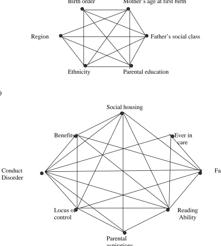
Figures 4a to 4c show the independence graphs for the first three steps of the analysis. Apart from birth order, all of the block 1 variables are mutually dependent (Figure 4a). Figure 4b shows that, at age 10, social housing, receipt of benefits, family structure, conduct disorder, reading ability and locus of control are mutually dependent. Ever having been in statutory care is associated with conduct disorder, reading ability and family structure, but is conditionally independent of the rest of the block 2 variables, given these three variables and the block 1 variables. The chain graph in Figure 4c depicts the significant inter-block

associations between blocks 1 and 2. Father’s social class has a direct, possibly causal, association with all of the block 2 variables, reflecting the strong continuity in social disadvantage between birth and childhood. Parental education and mother’s age at first birth are directly related to the risk of living in social housing at age 10. Socio-economic circumstances at birth are also directly related to the child’s individual attributes at age 10. Father’s social class, parental education and mother’s age at first birth all have direct, potentially causal, associations with the respondent’s reading ability, whilst father’s social class and parental education have a direct relationship with conduct disorder at age 10. Locus of control is dependent upon father’s social class, mother’s age at first birth and ethnicity, but is independent of parental education given the other variables in the first and second blocks.

Parental expectations that the child will leave school at age 16 are more common for children from manual or unsupported class backgrounds, those whose parents had themselves left school at 16 or before, those whose mothers became young parents, and those who were a second or higher order birth. Coming from a non-White background is related to an increased likelihood of receiving benefits, low reading ability, conduct disorder, having an external locus of control, and not living with two biological parents at age 10. After controlling for socio-economic circumstances, non-white children remain significantly more likely to experience statutory care4.

4

Figure 4: Independence graphs for the first three blocks (a) parental characteristics – intra-block associations; (b) childhood characteristics - intra-block associations; (c) socio-economic background factors prior to age at parenthood – inter-block associations

(a)

Birth

order

Mother’s

age

at

first

birth

Region

Father’s social class

Ethnicity

Parental

education

(b)

Social

housing

Benefits

Ever in

care

Conduct

Family structure

Disorder

Locus of

control

Reading

Ability

(c)

Ethnicity Mother’s age Father’s social Birth Parental Region

first birth class order education

Benefits Family Reading Locus Conduct Parental Social Ever in Structure ability of control disorder aspirations housing care

The chain graph in Figure 4c includes arrows linking region with a number of childhood circumstances and characteristics. However, all of the latter relationships, although statistically significant, are substantively very small and are not discussed further. Besides direct associations, all variables in the first block have indirect associations with variables in the second block. For example, parental education has an indirect association with receipt of benefits at age 10, since there is a path made up of a line (undirected edge) between parental education and father’s social class (see Figure 4a) and an arrow (directed edge) between father’s social class and receipt of benefits (see Figure 4c).

Figure 5 contains the chain graph depicting the pathways through which parental and childhood

characteristics are related to age at motherhood. In order to make the chain graph easier to read by reducing the number of edges displayed some variables within a block have been rearranged into sub-blocks.

Figure 5: Chain graph for antecedents of age at motherhood

Birth order

Ethnicity Mother’s age Father’s social Parental Region

first birth class education

Ever in care

Benefits Family Reading Locus of Conduct

structure ability control disorder

Parental Social

aspirations housing

For example, father’s social class, maternal age at first birth and ethnicity are all dependent upon each other and are all directly associated with receipt of benefits, family structure and reading ability. Instead of drawing individual lines between each of the individual variables we summarize the association by drawing an arrow from the first sub-block in block 1 to a second sub-block in block 2. When not all of the variables in a sub-block are directly related to another variable (or block), a single edge is drawn between the variable in the first block and the second variable (or sub-block). For example, father’s social class and ethnicity are related to experience of statutory care, but mother’s age at first birth is not. Therefore, we draw two arrows, one linking father’s social class and experience of statutory care, and one linking ethnicity and experience of statutory care.

Inspection of the chain graph in Figure 5 tells us that mother’s age at first birth, father’s social class, parental education, and region all have a direct association with age at motherhood, indicated by the arrows from these variables to block 3. These parental background factors also have an indirect relationship with age at motherhood through their association with childhood characteristics. In fact, all of the childhood characteristics, apart from experience of statutory care and locus of control are directly associated with age at motherhood. Experience of statutory care is indirectly associated with age at motherhood through its association with conduct disorder, reading ability and family structure, whilst locus of control is indirectly associated with age at motherhood because of its association with all of the other childhood variables (apart from experience of care).

Age at motherhood is conditionally independent of ethnicity given the other variables in blocks 1 and 2. In other words ethnic differences in age at motherhood are mediated by the poorer socio-economic backgrounds of non-white women and their subsequent childhood characteristics.

Figure 6: Chain graph for antecedents of less than good health

Birth order

Ethnicity Mother’s age Father’s social Parental Region

first birth class education

Ever in care

Benefits Family Reading Locus of Conduct

structure ability control disorder

Parental Social

aspirations housing

Age at motherhood

Partnership dissolution

Person to confide in

No work Social No other

family housing adult

Close to Satisfied mother with area

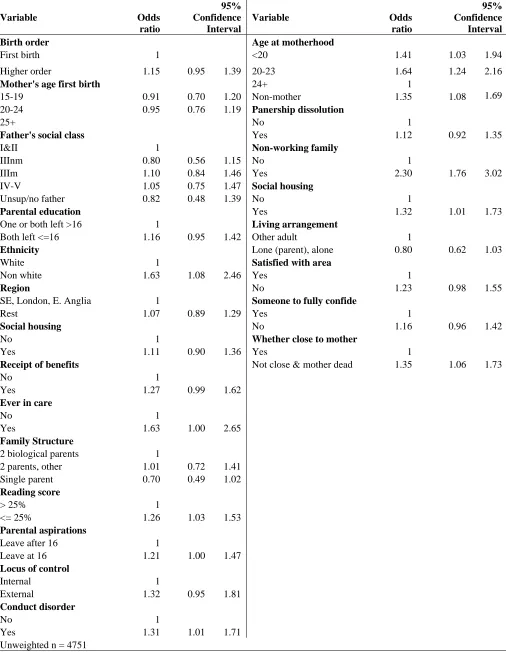
Table 1: Odds ratios from logistic regression models of self-reported health status at age 30.

Variable Odds

ratio

95% Confidence Interval

Variable Odds

ratio

95% Confidence Interval

Birth order Age at motherhood

First birth 1 <20 1.41 1.03 1.94

Higher order 1.15 0.95 1.39 20-23 1.64 1.24 2.16

Mother's age first birth 24+ 1

15-19 0.91 0.70 1.20 Non-mother 1.35 1.08 1.69

20-24 0.95 0.76 1.19 Panership dissolution

25+ No 1

Father's social class Yes 1.12 0.92 1.35

I&II 1 Non-working family

IIInm 0.80 0.56 1.15 No 1

IIIm 1.10 0.84 1.46 Yes 2.30 1.76 3.02

IV-V 1.05 0.75 1.47 Social housing

Unsup/no father 0.82 0.48 1.39 No 1

Parental education Yes 1.32 1.01 1.73

One or both left >16 1 Living arrangement

Both left <=16 1.16 0.95 1.42 Other adult 1

Ethnicity Lone (parent), alone 0.80 0.62 1.03

White 1 Satisfied with area

Non white 1.63 1.08 2.46 Yes 1

Region No 1.23 0.98 1.55

SE, London, E. Anglia 1 Someone to fully confide

Rest 1.07 0.89 1.29 Yes 1

Social housing No 1.16 0.96 1.42

No 1 Whether close to mother

Yes 1.11 0.90 1.36 Yes 1

Receipt of benefits Not close & mother dead 1.35 1.06 1.73

No 1

Yes 1.27 0.99 1.62

Ever in care

No 1

Yes 1.63 1.00 2.65

Family Structure

2 biological parents 1

2 parents, other 1.01 0.72 1.41

Single parent 0.70 0.49 1.02

Reading score

> 25% 1

<= 25% 1.26 1.03 1.53

Parental aspirations

Leave after 16 1

Leave at 16 1.21 1.00 1.47

Locus of control

Internal 1

External 1.32 0.95 1.81

Conduct disorder

No 1

Yes 1.31 1.01 1.71

Figure 6 shows the pathways through which age at motherhood and other variables in blocks 1, 2 are associated with the risk of partnership dissolution, circumstances in adulthood, and ultimately, self reported health at age 30. In order to simplify the presentation, only edges leading to variables in blocks 4, 5 and 6 are depicted. The graph can be read in conjunction with Table 1 which gives the odds ratios from a separate logistic regression model of self reported health at age 30 with the variables in blocks 1 to 5 entered as explanatory variables5. The odds ratios in Table 1 provide us with information about the ways in which categories of the explanatory variables are related to health at age 30, but only provide estimates of the direct or net effects. In contrast, the graphical model depicts the structure of relationships between all of the

variables in the data, and shows both the direct and indirect pathways through which parental background and childhood factors are associated with health in adulthood.

The chain graph in Figure 6 suggests that the probability of less than good health at age 30 is related to a wide range of factors experienced throughout the life course. Only one variable from block 1, ethnicity, has a direct relationship with health in adulthood. Even when all other factors are controlled ethnicity remains directly related to less than good health. The odds ratio in Table 1 suggests that non white women were 60% more likely to report less than good health. All of the other parental characteristics and birth circumstances are associated with less than good health at age 30 via their impact on childhood circumstances (particularly low reading ability, conduct disorder, parental expectations and experience of statutory care) and later life course experiences (particularly age at motherhood and poverty in adulthood). Reading ability and conduct disorder have direct relationships to poor adult health. These childhood factors are joined by parental expectations for the age at which their child will leave school and experience of institutional care which are also directly related to poor adult health. It is clear that experience of economic disadvantage in childhood and in adulthood combine across the life course to create health inequalities. For example, low reading ability in childhood is associated with poorer health directly (odds ratio 1.3) and indirectly through the relationship between reading ability with other age 10 circumstances, a greater risk of young motherhood, a greater risk of being in a non-work family and in socially rented accommodation in adulthood. Women who are living in a non-work family are more than twice as likely to be in poorer health, whilst those living in social rented housing are 1.3 time more likely to report less than good health.

5

Experience of a partnership dissolution is not found in itself to be related to poor health, but is indirectly associated via poorer living conditions in adulthood and being less emotionally close to ones mother6. Neither satisfaction with their neighbourhood, nor having someone to fully confide in are significant predictors of overall general health.

Combining our results from Figures 5 and 6 we conclude that some of the observed univariate association between young motherhood and poor adult health is due to common antecedent factors. Young mothers are more likely to come from a poor socio-economic background and hence being more likely to have childhood characteristics such as conduct disorder, poor reading ability and experiences such as that of statutory care which are themselves associated with poorer health in adulthood. When these common antecedent factors are controlled, young motherhood remains associated with less than good health at age 30. The graphical model shows that in part this relationship is mediated through the poorer socio-economic circumstances in

adulthood of younger mothers, and their greater risk of being emotionally distant from their own mothers.

6. Conclusion

In this paper we demonstrated how graphical modelling can be used as an effective tool in life course research focusing in particular on longitudinal prospective data. Graphical models and chain graph models allow scientists to state clearly the conceptual framework on which the analysis is based and the assumed causal relationships amongst events. By breaking down large multivariate systems into simpler more

tractable subcomponents and analysing them via local regressions, graphical models helps the understanding of complicated life course processes, show the intermediate relationships between predictors and aid the understanding of the mechanisms through which potential confounding and mediating factors affect the outcome of interest. When longitudinal prospective data are used, the chain graph maintains the temporal ordering of events through the sequence of its components. This helps cope with attrition in the data as each regression can be run on the available data confining the potential more serious effect of the dropout to the

6

late stages of the modelling where the regressions can be combined with appropriate ways to handle attrition, for example, by weighting.

Structural equation models (SEM) have been using extensively for analysing multivariate data. Both SEM and graphical modelling can be seen has an extension of path analysis model (Wright, 1934). Graphical chain graph models can in some cases give an alternative interpretation of a structural equation system. The graph associated to a SEM however may not, in general, be a chain graph and the model will not have, in general, a chain graph interpretation (Lauritzen and Richardson, 2002). It has been shown (Koster 1999) how an independence graph can be associated with a structural equation model which represents all the

independence statements implied by the model. However, while in a chain graph each edge corresponds to a marginal or conditional association of a pair of variables and the lack of it always represents a conditional independence this does not hold in general for SEM. Graphical models extend path analysis models by allowing the modelling of both categorical and continuous variables and, to some extent, a mixture of them. Discrete variables entered as responses into a SEM are usually handled by assuming that they are generated by an underlying Gaussian variable whose support is partitioned to provide categories. This implies that nominal categorical variables cannot be properly accounted for in a SEM and that the interactive effect of two or more variables on the response cannot be represented (Cox and Wermuth 1996). Graphical modelling copes with discrete variables in a natural way and therefore seems more suitable for modelling social data which are often categorical.

References

Agresti, A. (2002) Categorical Data Analysis, Second Edition. Hoboken, New Jersey: John Wiley & Son. Breiman, L., Friedman, J.H., Olshen, R.A. and Stone, C.J. (1984) Classification and Regression Trees. Belmont, CA: Wadsworth and Brooks/Cole.

Borgoni, R. and Berrington, A. (2004) A tree based procedure for multivariate imputation. Proceedings of the XLII Conference of the Italian Statistical Society, forthcoming.

Clark L.A. and Pregibon D. (1992) Tree-Based Models in Statistical Models. In S. J. M. Chambers and T. J. Hastie (eds.). Pacific Grove, CA: Wadsworth & Brooks/Cole.

Cheesbrough, S. (2003) Young motherhood: Family transmission or family transitions? Pp 79-102 in G. Allan, and G. Jones (eds.) Social Relations and the Life Course. London: Palgrave Macmillan.

Cheung, S.Y. and Andersen, R. (2003) Time to read: family resources and education outcome in Britain.

Journal of Comparative Family Studies, 34, 413-433.

Cowell, R.G., Dawid, A.P., Lauritzen, S.L. and Spiegelhalter, D.J. (1999) Probabilistic networks and expert systems. New York: Springer-Verlag.

Cox, D.R. and Wermuth, N. (1996) Multivariate Dependencies: Models, Analysis and Interpretation. London: Chapman and Hall.

Edwards, D. (1989). Discussion on mixed graphical association models (by S.L Lauritzen). Scandinavian Journal of Statistics, 16, 301.

Edwards, D. (2000) Introduction to graphical modelling; 2nd edn. New York: Springer. Elder, G.H. (1985) Life Course Dynamics. Ithaca, NY: Cornell University Press.

Ferri, E., Bynner, J., and Wadsworth, M. (2003) Changing Britain, Changing Lives: Three generations at the turn of the century. University of London: Institute of Education.

Hobcraft, J. and Kiernan, K. (1999) Childhood poverty, early motherhood and adult social exclusion. Centre for Analysis of Social Exclusion Working Paper 28. London School of Economics.

Jaffee, S. (2002) Pathways to adversity in young adulthood among early childbearers. Journal of Family Psychology, 16, 38-49.

Koster, J.T.A. (1999) On the validity of the Markov Interpretation of path diagrams of gaussian structural equations systems with correlated errors. Scandinavian Journal of Statistics, 26, 413-431.

Lauritzen, S.L. (1996) Graphical Models. Oxford: Oxford University Press.

Lauritzen S.L. and Richardson T.S. (2002) Chain graph models and their causal interpretations, Journal of the Royal Statistical Society: Series B, 64, 321-361

Little, R.J.A. and Rubin, D.B. (2002) Statistical analysis with missing data, Second Edition. Hoboken, NJ: John Wiley & Son.

Magadi, M., Diamond, I., Madise, N. and Smith, P. (2004) Pathways of the determinants of unfavourable birth outcomes in Kenya. Journal of Biosocial Science, 36, 153-176.

Mohamed, W.N. (1995) The Determinants of Infant Mortality in Malaysia. PhD Thesis. Southampton: University of Southampton.

Mohamed, W.N., Diamond, I and Smith, P.W.F. (1998) The determinants of infant mortality in Malaysia: a graphical chain modelling approach. Journal of the Royal Statistical Society Series A, 161, 349-366. Office for National Statistics (2000) Health in England 1998: Investigating the links between social inequalities and health. London: The Stationery Office.

Pearl, J. (1995) Causal diagrams for empirical research, Biometrika, 82, 669-710.

Pearl, J. (2000) Causality: Models, Reasoning and Inference. Cambridge: Cambridge University Press. Power, C. and Manor, O. (1992) Explaining social class differences in psychosocial health among young adults: a longitudinal perspective. Social Psychiatry and Psychiatric Epidemiology, 27, 284-291.

Power, C., Stansfeld, S., Matthews, S. Manor, O. and Hope, S. (2002) Childhood and adulthood risk factors for socio-economic differentials in psychological distress: evidence from the 1958 British birth cohort.

Social Science and Medicine, 55, 1989-2004.

Venables, W.N. and Ripley, B.D. (2002) Modern Applied Statistics with S-PLUS. Fourth Edition. Springer Berlin.

Rotter, J. B. (1966) Generalized expectancies for internal versus external control of reinforcement.

Psychological Monographs, 80, 609.

Rutter, M., Tizard, J. and Whitmore, K. (1970) Education, Health and Behaviour. London: Longmans. Sacker, A., Schoon, I. and Bartley, M. (2002) Social inequality in educational achievement and psychosocial adjustment throughout childhood: magnitude and mechanisms. Social Science and Medicine, 55, 863-800. Wermuth, N. and Lauritzen, S.L. (1990) On substantive research hypotheses, conditional independence graphs and graphical chain models (with discussion), Journal of the Royal Statistical Society, Series B, 52, 21-72.

Wermuth, N. (1993) Association Structures with few variables: characteristics and examples, In K. Dean (ed.) Population Health Research Linking Theory and Methods, London: Sage Publications.

Appendix 1

Estimation of Attrition Weights

In this appendix we describe the estimation of the attrition weights used in the final regression model. Since we required substantive information on the parental background and birth characteristics of those born in Britain in 1970 we excluded from the sample all cohort members not present in the original birth survey. Furthermore, we disregard those who were not present at age 10 when the childhood characteristics were measured, even if they rejoined the study sample at age 30. This results in a monotone attrition structure which permits the use of weights in order to re-proportion the sample to the original size.

Attrition indicators for missing data were defined for the age ten sweep (M10) and the age 30 sweep (M30). The first missing indicator takes value 0 if a woman originally in the sample is also observed at age 10 and 1 if she dropped out. The second attrition indicator takes value 0 if an individual was in a sample at age 10 and age 30, and 1 if she dropped out by age 30. This second attrition indicator is not defined for women missing at age 10. Our sample consists of 7392 respondents born in Britain who took part in the birth survey. Of these, 6249 respondents were still in study at age 10, whilst 1143 dropped out. Among those still in the study at age 10, 4766 were also observed at age 30. Table A.1 summarises the situation.

Table A.1: Summary of Response of BCS70 Females Sweep

Whether took part Birth Age 10 Age 30

Yes 7392 6249 4766

No 0 1143 2626

The probability that a unit is in the sample both at age 10 and age 30 is then:

Pr{M30=0, M10=0} = Pr{M30=0 | M10=0} × Pr{M10=0} (1)

Our aim is to estimate the two probabilities on the right-hand side of equation 1. We assume that the drop-out mechanism is missing at random given a set of observed predictors. Let X0 be the vector of variables

which predict attrition between birth and age 10 and let X10 be the vector of covariates predicting loss

between age 10 and 30. In this way we create a number of weighting classes. For each of these classes we estimate the probability of response. The weight is then the reciprocal of the two combined probabilities:

W=1/ Pr{M30=0, M10=0| X0 X10}=1/[ Pr{M30=0| X0 X10, M10=0}×Pr{M10=0| X0}] (2)

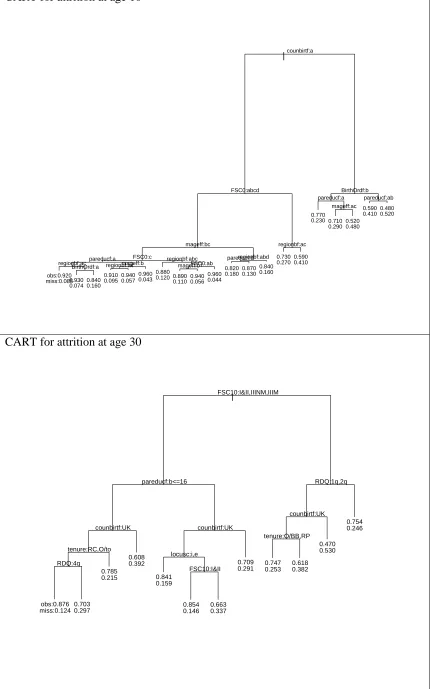
In our case all of the predictors are categorical. We use a semiparametric approach known as a classification tree to identify the adjustment classes and their probabilities of response. Explanatory variables entered into the first tree modelling response at age 10 include: birth order, region of birth of the cohort member (CM), parental education, father’s social class at birth, country at birth of the CM’s mother, age at first birth of the CM’s mother. All the predictors were measured at birth.7 The tree was grown allowing a node to be split only if it contained at least 70 units.

A second classification tree was then grown on the subsample of people observed at age 10 (M10=0). For this tree the response is M30 and the predictors are: birth order, parental education, father’s social class at age 10, country at birth of the CM’s mother, age at first birth of the CM’s mother, housing tenure at age 10, and the child’s locus of control and reading score at age 10. The tree was grown allowing a node to be split only if it contained at least 60 units.

7

Since the product of the two sets of probabilities produced a large number of weighting classes, some of them characterised by a very small count, the number of classes was reduced by collapsing neighbouring classes together. The weight of the new category was calculated as the weighted average of the weights in the two original classes, the weights of the mean being the share of the people in each of the two categories.

A brief review of classification trees

Classification and regression trees have been used extensively in statistics since the seminal book of Breiman et al. (1984). A classification tree aims to partition the sample space into a number of classes and to allocate each observation into one of these classes. The classification rule is based on a sample of data, called a learning or training set, of units for which the actual classification is available. The partition of the space is provided by the terminal nodes or leaves of the tree and for each terminal node the probability distribution across the response categories is obtained.

Construction of the tree consists of defining a measure of homogeneity or variability of the distribution at a node and splitting the sample falling into that node in the way which produces the largest reduction in the average variability. Many of the algorithms used for tree construction choose the next split in an optimal way and do not aim to optimise the performance of the whole tree. In particular many algorithms proceed by binary splits which facilitate comparisons between alternative splits. For categorical variables the Gini index or the Shannon’s entropy are usually used as measure of homogeneity of nodes. The splitting procedure continues until a minimum number of cases fixed in advance are contained in the current node or the node is homogenous enough, i.e. the reduction in the average variability is below a given threshold.

It is standard practice in building trees initially to construct initially a large model and then to reduce it without sacrificing goodness of fit. This can be obtained by using two procedures known as pruning and shrinking. Shrinking consists of pulling back the probabilities in the terminal nodes toward the root. The pruning consists of removing from the tree those subtrees originated by less important splits according to a cost-complexity measure. In order to obtain robust results it is good practice to use a different dataset from the one used to grow the tree. If a validation set is not available one can be made by splitting the sample in two parts and use one as training set and the other as validation set (or by using a more computational intensive k-fold cross-validation procedure).

Many software are nowadays equipped with tools for building trees and this has largely contributed to the spread of this technique in recent years. In this analysis we use the function TREE available in SPLUS 2000 (Clark and Pregibon, 1992; Venebles and Ripley, 2002).

Implementation technicalities

In order to avoid problems of overfitting (i.e. the tree tending to fit the data too well identifying very specific and small clusters which depend on the specific dataset more than on the underlying process), the sample was split into two sub-samples. The first one, the training set, consisted of 60% of the data (4400

observations) and was used to estimate the two trees. The second one (2992 observations) called the test or validation set was used to check them. A tree larger than necessary was initially grown and then pruned back keeping the best 20terminal nodes for the classification tree of non-response at age 10 and the best 12 terminal nodes for the classification tree of non-response at age 30. The number of nodes to be used in the optimal pruning of the tree is determined by picking out the value which maximises the correlation

coefficient between the estimated probability of response in each terminal nodes and the observed one. This search is done using the test set in order to obtain a robust model. For the tree predicting response at age 10 the correlation coefficient (weighting the observed and the estimated probability in each group by the number of people classified in the group) was 0.84. For the tree predicting response at age 30 the weighted correlation coefficient was 0.80.

birth were not retained in the tree for attrition between age 10 and age 30. The two trees are reported in Figure A.1.

There were a very small number of units with item non-response in some of the predictors. These records were kept in the analysis. Cases with item non-response are dropped down the tree until a leaf or node was reached for which the attribute was missing. If the node is not a leaf the probability of attrition for those observations was calculated using the empirical probability provided by this node. This means that the number of adjustment classes in each tree is not exactly equal to the leaves of the tree since some extra categories were identified by these intermediate nodes.

The joint predicted probability of response at age 10 and 30 was then computed. In the test dataset this product produced 81 weighting classes, many of them containing few people (for example, 35 groups have less than 10 cases). The number of weighting classes was then reduced by constraining a minimum

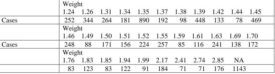
weighting class size. In order to determine this minimum size the weighted correlation coefficient between the observed and predicted vectors of probabilities of response was estimated and plotted against the minimum class size. We choose the class size for which the curve achieves its maximum, restricting our search to sizes below 85 to avoid the situation where a very high correlation coefficient is actually due to a small number of classes with large frequencies. As Figure A.2 shows, this curve achieves its maximum at 70. This minimum size guarantees 20 weighting classes.

Figure A.1

CART for attrition at age 10

|counbirtf:a FSC0:abcd mageff:bc FSC0:c pareducf:a regionbf:ac

BirthOrdf:a regionbf:acmageff:b

regionbf:abc FSC0:ab mageff:b regionbf:abd pareducf:b regionbf:ac BirthOrdf:b pareducf:a mageff:ac pareducf:ab obs:0.920 miss:0.0850.930 0.074 0.840 0.160 0.910 0.0950.9400.057

0.960 0.043 0.880 0.120 0.890 0.110 0.940 0.056 0.960 0.044 0.820 0.1800.8700.130

0.840 0.160 0.730 0.270 0.590 0.410 0.770 0.230 0.710

0.2900.5200.480 0.590 0.410

0.480 0.520

CART for attrition at age 30

| FSC10:I&II,IIINM,IIIM pareducf:b<=16 counbirtf:UK tenure:RC,O/to RDQ:4q counbirtf:UK locusc:i,e FSC10:I&II RDQ:1q,2q counbirtf:UK tenure:O/BB,RP obs:0.876 miss:0.124 0.703 0.297 0.785 0.215 0.608 0.392 0.841 0.159 0.854 0.146 0.6630.337

0.709 0.291 0.7470.253

Figure A.2: Weighted correlation coefficient between the observed and predicted vectors of probabilities of response plotted against the minimum class size

min. adjusting categories size

correlat

ion coef

fi

cient

20 30 40 50 60 70 80

0.

70

0.

72

0.

74

0.

76

0.

78

0.

80

Table A.2: Final weights from whole dataset for response at age 30 Weight

1.24 1.26 1.31 1.34 1.35 1.37 1.38 1.39 1.42 1.44 1.45 Cases 252 344 264 181 890 192 98 448 133 78 469 Weight

1.46 1.49 1.50 1.51 1.52 1.55 1.59 1.61 1.63 1.69 1.70 Cases 248 88 171 156 224 257 85 116 241 138 172 Weight