Numerical Construction of Parameter Maximin
D-Optimal Designs for Binary Response Models
Stefanie Biedermann
Ruhr-Universit¨at Bochum
Fakult¨at f¨
ur Mathematik
44780 Bochum
Germany
email: [email protected]
Holger Dette
Ruhr-Universit¨at Bochum
Fakult¨at f¨
ur Mathematik
44780 Bochum
Germany
email: [email protected] FAX: +49 2 34 70 94 559
April 13, 2005
Abstract
For the binary response model, we determine optimal designs based on theD-optimal criterion which are robust with respect to misspecifications of the unknown parameters. We propose a maximin approach and provide a numerical method to identify the best two point designs for the commonly applied link functions. This method is broadly applicable and can be extended to designs with a given number (≥2) of support points and further link functions. The results are illustrated for the logistic and probit model, for which several examples of maximin D-optimal designs are calculated explicitly by our method.
Keywords and Phrases: Binary response model, robust optimal design, maximin D-optimality, Bayesian D-optimality, prior distribution
1
Introduction
We consider the common binary response model where a subject is administered a stimulus at a dose level x ∈ IR. The response X is a binary random variable with success probability
p(x, ϑ), i.e. X ∼ Bin(1, p(x, ϑ)), wherex∈IRis the explanatory variable andϑis an unknown parameter. In this article, we deal with the following parametrization of a two parameter binary response model,
p(x, ϑ) =F(β(x−µ)), ϑ= (µ, β)T, µ ∈IR, β ∈IR+,
where F denotes a known distribution function with density f. For this model the Fisher information for the parameter ϑ at a point x is given by
I(x, ϑ) =h(β(x−µ)) β
2 −β(x−µ)
−β(x−µ) (x−µ)2
!
,
where the functionh(z) is defined as
h(z) = f
2(z)
F(z)(1−F(z)). (1.2)
An (approximate) design ξ is a probability measure with finite support on IR,i.e. the observa-tions are taken at the support points of the measure proportional to the corresponding masses. The Fisher information of the designξ is given by
M(ξ, ϑ) =
Z
I(x, ϑ)dξ(x),
(1.3)
and an optimal design maximizes a real-valued function of the Fisher information matrix, which is usually referred to as an optimality criterion [see e.g. Silvey (1980)]. A typical example is
D-optimality where the determinant of the Fisher information is maximized with respect to the design ξ, thus minimizing the (first order approximation of the) volume of the ellipsoid of concentration for the parameterϑ.
Much effort has been devoted to the problem of finding good designs for the binary response model [see Kalish and Rosenberger (1978), Abdelbasit and Plackett (1983), Minkin (1987), Sitter and Fainaru (1997) among many others]. Since the Fisher information and thus theD -optimal design depends on the unknown parameter aD-optimal design cannot be implemented directly in practice. Following Chernoff (1953), numerous authors assume that an initial guess of ϑ is available and determine so-called locally optimal designs [see Ford, Torsney and Wu (1992), Sitter and Wu (1993)]. However, misspecifications of the parameter can lead to poor results in the subsequent data analysis. A more robust alternative is to assume sufficient knowledge ofϑ to specify a prior distribution for this parameter and to average the respective optimality criteria over the plausible values of ϑ defined by the prior. This leads to so-called Bayesian optimality criteria [see e.g. Chaloner and Larntz (1989)].
As an alternative for the construction of robust designs, we propose a maximin approach based on the D-optimality criterion, which only requires the specification of a certain range for the unknown parameters. We feel that this is a more realistic scenario since practitioners will often have difficulties in specifying a prior distribution for the unknown parameterϑ, especially if this is multidimensional. So far, maximin D-optimal designs have been found only within a very restricted class of designs, i.e. equidistant designs with equal weights and symmetric about the mean of the µ-interval [see Sitter (1992)]. The main difficulty for the construction of optimal designs with respect to maximin optimality criteria is the non-differentiability of this type of criteria. We solve this problem by exploiting the close relation between Bayes- and maximin optimality criteria [see Dette, Haines and Imhof (2004)]. This allows us to obtain the maximin
In Section 2, we describe the above optimality criteria, the method for the construction of maximin optimal designs and its implementation considering minimally supported designs. Several examples of link functions are given, for which the method works without modifications. Section 3 deals with extensions of the method to the other commonly applied link functions as well as designs with more than two support points. In Section 4, the minimally supported designs from Section 2 are taken up again and investigated with respect to global optimality (i.e. optimality within the class of all designs). Finally, some of the more technical arguments are deferred to an appendix.
2
Maximin
D
-optimal two point designs in the binary
response model
In the following, we motivate and define the optimality criterion under consideration in this article. As indicated in the introduction, D-optimal designs depend on the unknown model parameters and are not necessarily robust with respect to their misspecification. There are two non-sequential approaches to constructing optimal designs based on theD-criterion, which are more robust. On the one hand, it can be reasonable to assume that some prior knowledge about the parameter ϑ is available in advance, which can be specified by a probability distribution on the parameter space Θ. In such cases it makes sense to choose a design that maximizes a function of the determinant of the information matrixM(ξ, ϑ) after averaging out the plausible values ofϑby a prior distribution, say ˜π. Since the use of standardized criteria is recommended to avoid different scalings [see Dette and Wong (1996) or Dette (1997)] this leads to a Bayesian optimality criterion based on the D-efficiencies
effD(ξ, ϑ) =
|M(ξ, ϑ)|
|M(ξϑ, ϑ)| 1/2
,
where ξϑ denotes the locally D-optimal design for the parameter ϑ. The criterion function
˜
Ψp(ξ) is then defined as
˜ Ψp(ξ) =
" Z
Θ
|M(ξ, ϑ)|
|M(ξϑ, ϑ)| p/2
dπ˜(ϑ)
#1p
, − ∞< p <0,
(2.1)
and a Bayesian ˜Ψp-optimal designξ with respect to the prior ˜π maximizes this expression over
the set of all approximate designs on the design space [see Dette and Wong (1996)]. Equivalently, we will use a simplified notation for this criterion, where each prior distribution ˜π is identified with an associated priorπ defined by
dπ(ϑ) =|M(ξϑ, ϑ)|−qdπ˜(ϑ)
replacing the expression p/2 by q. A monotone transformation of the standardized Bayesian
D-optimality criterion function can then be written as
Ψq(ξ) = hZ
Θ|
M(ξ, ϑ)|qdπ(ϑ)i 1 q
If, on the other hand, the specification of a prior distribution π on the parameter space is not possible in advance, it is sensible to construct the design for the protection of the experiment against the worst possible case, i.e. against the values of ϑ ∈ Θ minimizing the D-efficiency. In this case the optimal design maximizes the minimal D-efficiency with respect to Θ which yields the standardized maximin D-optimality criterion
Ψ−∞(ξ) = inf
ϑ∈Θ
|M(ξ, ϑ)|
|M(ξϑ, ϑ)| 1/2
(2.2)
[see M¨uller (1995) or Imhof (2001)]. Throughout this article, we call a design maximizing the above function Ψ−∞-optimal (with respect to Θ), where Θ denotes the space of possible values
for the parameter ϑ. Obviously, in the maximin case it is not necessary to have as much prior knowledge to specify certain preferable values forϑas is needed in the Bayesian case. The only ”parameter” the experimenter has to choose in advance is the ”region of uncertainty” Θ as a subset ofIR×IR+. Note that the standardized maximin criterion is obtained in the limit from
the Bayesian criterion asq tends to− ∞. For this reason, the notation Ψ−∞ is consistent with
the above definitions. It is easy to see that in the binary response model with parametrization (1.1) the value of the optimal determinant of the Fisher information matrix|M(ξϑ, ϑ)|does not
depend on the value of the parameter vector ϑ ∈ Θ, i.e. the standardization of the criterion function is constant with respect toϑ.Therefore we will use the notation ”maximinD-optimal” as equivalent to ”standardized maximin D-optimal” as well as the analogous notation for the Bayesian case in what follows. Of course the D-optimal design ξϑ is parameter dependent.
A computational advantage of the Bayesian optimality criterion is its Fr´echet differentiability. As a consequence, standard numerical methods for the determination of Bayesian D-optimal designs can easily be adapted [see e.g. Chaloner and Larntz (1989)]. The determination of maximin D-optimal designs, however, is a substantially more complex problem. Usually the structure of the particular design criterion under consideration has to be used for the con-struction of algorithms [see Sitter (1992) or Fandom Noubiap and Seidel (2000)]. We will now discuss a general strategy to obtain maximin optimal designs as limits from Bayesian optimal designs.
From Theorem 2.1 in Dette, Haines and Imhof (2004) we obtain a close connection between Bayesian and maximin optimal designs, which we will use to construct maximin D-optimal designs from their Bayesian counterparts. The first part of the following theorem reports a special case of the above-mentioned result, so that it is applicable for our purpose. Part two, moreover, deals with a simplification with respect to the choice of the prior π, which will be exploited in subsequent material to simplify our method.
Theorem 1
1. Let Θ be compact and for every q ≤ 0, let πq be an arbitrarily chosen prior distribution
on Θ. Denote by ξq a Bayesian Ψq-optimal design with respect to the prior πq within a
class of designs ∆ and suppose that the following conditions hold.
(b) The class of Bayesian Ψq-optimal designs {ξq | q ≤ 0} is tight and its closure is
contained in ∆.
(c) There is a finite measureπ onΘwith supportsupp(π) equal toΘsuch that for every measurable subset T ⊂Θ with π(T)>0,
lim inf
q→−∞ πq(T)>0.
Then the standardized Bayesian D-optimal designsξq converge weakly to some limit ξ∗ ∈
∆ as q→ −∞ and ξ∗ is standardized maximin D-optimal within the class ∆.
2. Let
N(ξ) = nϑ∈Θ|Ψ−∞(ξ) =
|M(ξ, ϑ)|
|M(ξϑ, ϑ)| 1/2o
.
If a superset E of N(ξ∗)is known, the above result still holds if we choose a finite prior π
on E withΘ⊃supp(π) =E ⊇ N(ξ∗) instead of a sequence{π
q}q≤0 onΘ, which satisfies
condition (c).
Remark 2
• The introduction of priors which may depend on the index q gives the statistician extra flexibility to simplify the numerical calculations to obtain the Bayesian optimal designs. In the following, however, we will use a sequence {πq}q≤0 that is constant with respect to
q, i.e. πq =π for all q ≤0, for simplicity.
• If condition (a) is not satisfied there may exist sequences of Bayesian optimal designs which converge to different limits. From the proof of Theorem 2.1 in Dette, Haines and Imhof (2004) it follows that any such limiting design is standardized maximin D-optimal within ∆.
• For further information on the conditions for convergence we refer the interested reader to Dette, Haines and Imhof (2004).
• The support of a probability measure ν is defined as follows
supp(ν) ={y | ν((−δ+y, y+δ))>0 ∀δ >0}.
Note that for a discrete measure ν the support is the set of points, which are given positive weight byν. To avoid possible confusion about the terms ”support of a prior” and ”support of a design” we note that a prior π (or πq) is a probability measure on the design space
Θ whereas a design ξ is a probability measure on the design interval, which is assumed to be the entire real axis in this article.
Theorem 3 Let Θ be convex. If the function h(z) in (1.2) is strictly log-concave and twice differentiable on IR, then for all equally weighted two point designs ξ the determinant |M(ξ, ϑ)|
is a strictly unimodal function with respect to ϑ.
The term ”strictly unimodal” in this context means that |M(ξ, ϑ)| features at most one local maximum with respect to the choice of parameter values, and no other local extremum. Strict log-concavity of a twice differentiable function g : IR→ IR means that the second derivative of logg is strictly negative so that functions which are constant with respect to some direction are excluded. In higher dimensions this is equivalent to the eigenvalues of the Hessian of logg
being strictly negative.
It follows from Ford, Torsney and Wu (1992) that the value of the optimal determinant of the Fisher information matrix M(ξϑ, ϑ) does not depend on the value of the parameterϑ∈Θ, and
as a consequence the standardization of the criterion function is constant with respect to ϑ.
For this reason, strict log-concavity of the function h(z) also implies strict unimodality of the standardized determinant function ||MM((ξξ,ϑ)|
ϑ,ϑ)| ifh(z) is twice differentiable and thusN(ξ
∗)⊂∂Θ,
[image:6.612.59.525.343.491.2]where ∂Θ denotes the boundary of the region of uncertainty. For the sake of brevity, we will refer to log-concavity and unimodality in the following when the strict versions of these properties are meant.
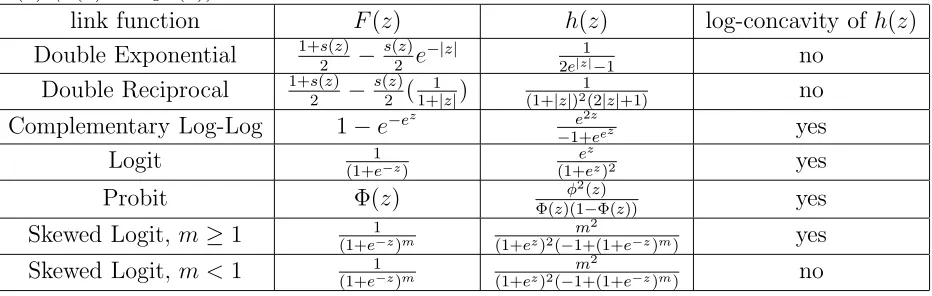
Table 1: Results on the log-concavity of the function h(z) for several common link functions
F(z) (s(z) =sign(z)).
link function F(z) h(z) log-concavity ofh(z) Double Exponential 1+s2(z) −s(2z)e
−|z| 1
2e|z|−1 no
Double Reciprocal 1+s2(z) − s(2z)( 1 1+|z|)
1
(1+|z|)2(2|z|+1) no
Complementary Log-Log 1−e−ez e2z
−1+eez yes
Logit (1+1e−z)
ez
(1+ez)2 yes
Probit Φ(z) Φ(z)(1φ2(−zΦ() z)) yes Skewed Logit, m ≥1 1
(1+e−z)m m 2
(1+ez)2(−1+(1+e−z)m) yes
Skewed Logit,m < 1 (1+e1−z)m m 2
(1+ez)2(−1+(1+e−z)m) no
Some of the commonly applied link functions and the information concerning the log-concavity of the corresponding functions h(z) are displayed in Table 1. It is interesting to note that the size of the parametermin the skewed logit model determines if the functionh(z) is log-concave. Most of the proofs of log-concavity for different functions h(z) including the tricky one for the probit link are given in Wu (1988).
The next theorem gives sufficient conditions for the function h(z) and the parameter region Θ such that the D-optimal two point design is unique.
We are now ready to outline a numerical method to calculate the maximinD-optimal two point designs for binary response models with parametrization (1.1). From a practical point of view it is reasonable to assume that the experimenter can specify a certain range for the position of either parameter before the experiment. This information leads to a rectangular subset of
IR×IR+ for Θ, i.e. Θ = [µ
1, µ2]×[β1, β2]. One might also think of parameter spaces which are
rectangular in µand log(β) given thatβ is the reciprocal of a standard deviation. Since the log-transformation is strictly monotonic this is equivalent to using a rectangle Θ = [µ1, µ2]×[ ˜β1,β˜2]
where ˜β1 =eβ1, β˜2 =eβ2. The following result relates maximinD-optimal designs with respect
to various rectangles and yields a substantial simplification of the optimization problem.
Lemma 5 Let ξ∗ denote the maximin D-optimal design for the binary response model (1.1) with respect to the parameter space Θ = [µ1, µ2]×[β1, β2] and c >0, ∆∈IR. The standardized
maximin D-optimal design ξ∗∗ with respect to the parameter space
˜
Θ =hµ1+ ∆
c ,
µ2+ ∆
c
i
×[cβ1, cβ2]
is given by
ξ∗∗({x}) =ξ∗({cx−∆})
where ξ({x}) denotes the weight that the design ξ assigns to the point x.
From Theorem 3 it follows that if the functionh(z) is log-concave and twice differentiable then for all equally weighted two point designs ξ the minimum of the D-efficiency of ξ over ϑ ∈ Θ can only be attained in the vertices of Θ, i.e.
N(ξ)⊆ {(µ1, β1),(µ1, β2),(µ2, β1),(µ2, β2)}.
We can now use Theorem 1 for the construction of maximinD-optimal two point designs, where
E denotes the set of the vertices of Θ and a priorπonEcan be chosen arbitrarily with positive weight for each vertex. Theorem 1 suggests that for all such priors π the maximin D-optimal two point design can be calculated as the limit of the Bayesian D-optimal two point designs with respect toπ whereq tends to− ∞.
For computational reasons, we chooseπ to be the uniform distribution onE. Thus the Bayesian
D-optimal two point designξq (with respect to the priorπ) can easily be computed numerically
maximizing the function
X2
i=1 2
X
j=1
1
4(|M(ξ, µi, βj)|)
q 1 q
.
(2.3)
We start with an initial value for q < 0, e.g., q0 = −100, calculate ξq0 and ξq1, where ql =
q0 ·10l, l = 0,1,2, . . ., and compare the respective values of the support points x1(qj) and
x2(qj) of the designsξq0 and ξq1. If both absolute distances are less than some threshold value,
e.g. 10−4 or 10−5, we propose to use ξ
q1 as an approximation to the maximin D-optimal two
so on. Usually four (or even less) steps of this procedure are sufficient to obtain the maximin
D-optimal two point design with high accuracy.
It is not possible to show that the Bayesian D-optimal two point designs ξq are unique in all
circumstances but given convergence we will always get a unique maximinD-optimal two point design [see Theorems 1 and 4]. If the sequence of BayesianD-optimal designs does not converge as q → − ∞ we propose to change the prior π to another distribution ¯π on E and start the procedure again. We would like to point out, however, that we calculated numerous examples, and we always observed convergence of the algorithm for whatever prior had been chosen. As the function (2.3) is defined as a weighted mean of four unimodal functions (due to the uniqueness of the locally optimal designs) we expect that there are not too many problems with respect to multimodality when carrying out the maximization step. Moreover, 3D-Plots of (2.3) with respect to different parameter spaces suggest that even this function will usually be unimodal itself in most cases. (In fact we did not find any situation in our examples where unimodality was not satisfied.) We recommend, however, to try different starting values for the maximization routine in case the algorithm is trapped at a local maximum (for some starting values), which is not global. This recommendation will be even more important when the extended algorithm described in the following section must be applied.
Recall that in the case of a log-concave and twice differentiable functionh(z) the worst case set
N(ξ) is a subset of the vertices of the parameter region Θ for all uniform two point designs ξ if the set Θ of parameters specified by the experimenter is a closed rectangle. If the condition of log-concavity ofh(z) is not fulfilled the above algorithm cannot be applied without modifications since we have no knowledge about the set N(ξ).The necessary modifications of our method in situations without log-concavity will be described in the next section.
Below, we give some examples of maximin D-optimal (two point) designs obtained by our method. We calculated the maximin D-optimal designs by the algorithm described in the previous paragraph. As mentioned before, the sequence of designs obtained by this algorithm converged to a limit in all cases under consideration in our study. We restrict ourselves to the logit and probit link functions only, to keep the length of this article in acceptable limits. The Maximin D-optimal two point designs for the logistic regression model with respect to several representative situations (concerning different parameter regions Θ; see column 1-4) are shown in the 5th and 6th column of Table 2. The next two columns of this table give the corresponding locallyD-optimal designs with respect to typical parameter values forµandβ given Θ, namely
µ and β are chosen as the arithmetic means of the intervals [µ1, µ2] and [β1, β2], respectively.
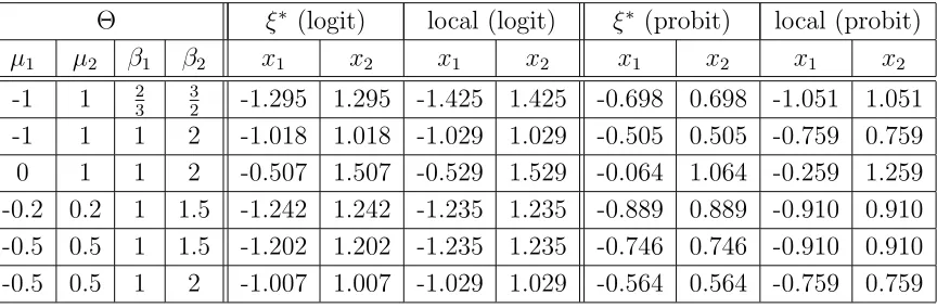
In the two right panels of Table 2 the corresponding designs for the probit model are listed. The support points of the respective designs are denoted by x1 and x2.
It is interesting to see that the locally D-optimal designs (with respect to the center of the rectangle) in the logistic regression model are rather close to the maximinD-optimal two point designs. Thus a practical recommendation for the optimal design of experiment in the logistic regression model is to use the locallyD-optimal design for the center ((µ1+µ2)/2,(β1+β2)/2))
of the parameter region Θ = [µ1, µ2]×[β1, β2], if Θ is not too large. On the other hand the
Table 2: MaximinD-optimal two point designs for the logit and probit link functions with respect to several parameter spaces. For comparison: The corresponding locally D-optimal designs with parameters µ= (µ1+µ2)/2, β = (β1+β2)/2.
Θ ξ∗ (logit) local (logit) ξ∗ (probit) local (probit)
µ1 µ2 β1 β2 x1 x2 x1 x2 x1 x2 x1 x2
-1 1 2 3
3
2 -1.295 1.295 -1.425 1.425 -0.698 0.698 -1.051 1.051
-1 1 1 2 -1.018 1.018 -1.029 1.029 -0.505 0.505 -0.759 0.759 0 1 1 2 -0.507 1.507 -0.529 1.529 -0.064 1.064 -0.259 1.259 -0.2 0.2 1 1.5 -1.242 1.242 -1.235 1.235 -0.889 0.889 -0.910 0.910 -0.5 0.5 1 1.5 -1.202 1.202 -1.235 1.235 -0.746 0.746 -0.910 0.910 -0.5 0.5 1 2 -1.007 1.007 -1.029 1.029 -0.564 0.564 -0.759 0.759
the maximin D-optimal two point designs and the locally D-optimal designs with respect to the center of the rectangle. The latter can be rather inefficient. Another plausible choice of µ
and β might be the arithmetic mean for µ and the geometric mean for β for the same reason as mentioned earlier in the discussion about using a log-scale for β. The locally D-optimal designs for these parameter choices, however, differ even more from the maximin D-optimal two point designs than the locally D-optimal designs with respect to the arithmetic means of both parameter intervals for both the logit and the probit links. This phenomenon occurs since the support points of the maximin D-optimal two point designs are (in particular for large
µ-intervals) closer to each other than the support points of the locally D-optimal designs with respect to the arithmetic means, which are given by xi =µa+zi∗/βa where µa and βa denote
the arithmetic means of the respective parameter intervals and z∗
i is a value depending only on
the underlying link function. The values ofz∗
i for the link functions discussed in this article can
be obtained from Table 4 in Ford, Torsney and Wu (1992). As the geometric mean is always less than the arithmetic mean the values of the points xi will be even more spread apart when
inserting the geometric mean of the β-interval in this formula, so that this design will be even further away from the maximin design. For the sake of brevity, the locally D-optimal designs with respect to (µ1+µ2)/2,√β1·β2), which can easily be calculated by the above formula from
Ford, Torsney and Wu (1992), are therefore not given in this article. We finally remark again that the maximin optimal designs given in Table 2 are optimal within the class of all two point designs. The discussion if these designs are optimal within the class of all designs is deferred to Section 4.
3
Extensions
h(z), which is satisfied for many but not all of the commonly applied link functions. In the following, we will briefly discuss how the method can be modified if the above conditions are not met. In these cases only the prior distribution on the parameter space Θ in the Bayesian optimality criterion has to be modified appropriately and the maximin optimal designs can again be obtained as limits from Bayesian optimal designs.
(a) Assume that Θ⊂IR×IR+is a convex, compact set, but not a rectangle (or polygon). If the
functionh(z) is log-concave we can chooseπ as the uniform distribution on the boundary of the set Θ. For computational reasons, this distribution should be approximated by an equidistant grid on the boundary of the set Θ.
(b) There are several cases where two point designs are not optimal and an efficient design
ξ with more than two support points is of importance. A typical example for such a situation appears if the optimal two point design is far from the globally optimal design (for a precise formulation see the next section), or if the design should also be used for model checking. Then even if the function h(z) is log-concave and twice differentiable the function |M(ξ, ϑ)| will in general not be unimodal with respect to ϑ for designs ξ with more than two support points. In this case we cannot specify a subset of the parameter space Θ containing N(ξ∗) and thus have to use the uniform distribution on Θ or its approximation on a grid as a prior in the Bayesian optimality criterion Ψq.
(c) If the function h(z) is not log-concave and twice differentiable and it cannot be shown that the minimum of |M(ξ, ϑ)| over Θ is attained at the boundary of Θ we also have to use the uniform distribution on Θ or its approximation by a discrete prior π.
Note that in all these cases the numerical procedure is applicable, where the only modification consists in the choice of the support for the prior distribution π on Θ. We calculate Bayesian Ψq-optimal designs and obtain the maximin optimal designs as limit as q→ −∞.However, an
additional amount of numerical calculation is required in such a situation because of the more complicated structure of the optimality criterion caused by the larger support of the prior π. We also used 3D-plots of Bayesian criterion functions with respect to several different priorsπ
for some fixed and two variable values of support points and weights of the underlying design to check if multimodality plays a role in respect of maximization. We found that even these more complicated functions seem to be unimodal. Since this can not be proven for general priors, we recommend to always check the optimality of a design by the equivalence theorem (Theorem 6, given in the following section). If the algorithm converges to a design which is not maximin optimal due to multimodality of the Bayesian criterion functions, the experimenter can choose a new starting value and apply the algorithm again. For all the examples in this article, we always observed convergence to the true maximin optimal design, which also suggests that multimodality is not a problem in this type of optimization problem.
strategy would therefore be to maximize in the class of symmetric designs with respect to this value and then check by the equivalence theorem if the result is in fact maximin D-optimal. This will reduce the number of free variables by about one half. Another idea emanates from the fact that the complexity of the prior π contributes to the complexity of the maximization problem. It might therefore be reasonable to start with a relatively coarse approximation π
to the uniform prior, then calculate the set N(ξ) of the resulting design ξ and check if this is contained in the support of π. If this is the case, the optimality of ξ can be checked by Theorem 6. Otherwise a new prior is formed with support on the union of supp(π) and N(ξ). This step will be repeated until a design ˜ξ is found with N( ˜ξ) a subset of the updated prior. Note that this strategy will not always lead to the maximin D-optimal design. The optimality of the resulting design must therefore be checked by an application of the equivalence theorem (Theorem 6).
4
Global Optimality and Efficiency
The designs found in Section 2 are maximinD-optimal within the class of all two point designs only. In this section, we will carefully analyze how they perform compared to the corresponding maximin D-optimal designs within the class of all designs. For the sake of brevity we call these designs also globally optimal. A powerful tool for checking optimality of a design is an equivalence theorem, which can be found in Dette, Haines and Imhof (2003).
Theorem 6 A design ξ∗ is maximin D-optimal with respect to Θ if and only if there exists a
prior π∗ supported on the set N(ξ∗) such that the inequality
d(ξ∗, x) =
Z
N(ξ∗)
trace{I(x, ϑ)M−1(ξ∗, ϑ)}dπ∗(ϑ)≤2 (4.1)
holds for all x∈IR.
Following Dette, Haines and Imhof (2003) we call the priorπ∗ the least favourable distribution.
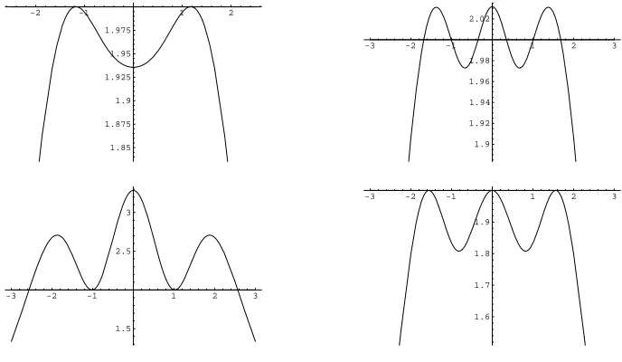
Checking optimality of the two point designs from Table 2 by the equivalence theorem indicates that designs corresponding to ”small” parameter spaces Θ tend to be more efficient than designs corresponding to a larger amount of uncertainty about the position of the unknown parameter. In our examples, the maximin D-optimal two point designs corresponding to the parameter spaces Θ = [−0.2,0.2]×[1,1.5] and Θ = [−0.5,0.5]×[1,1.5] turn out to be already optimal within the class of all designs. To give an illustration, Figure 1 shows the function d(ξ∗, x) from
the equivalence theorem for some two point designs and a three point design for the logistic regression model.
Figure 1: The function d(ξ∗, x) from the equivalence theorem for the logistic regression model.
Top left: The maximin D-optimal two point design with respect to Θ = [−0.5,0.5]×[1,1.5]
(globally Ψ−∞-optimal). Top right: The maximin D-optimal two point design with respect to
Θ = [−0.5,0.5]×[1,2] (almost globally Ψ−∞-optimal). Bottom left: The maximin D-optimal
two point design with respect to Θ = [−1,1]×[1,2] (far from global Ψ−∞-optimality). Bottom
right: The maximin D-optimal three point design with respect to Θ = [−1,1]×[1,2] (globally
Ψ−∞-optimal).
-2 -1 1 2
1.85 1.875 1.9 1.925 1.95 1.975
-3 -2 -1 1 2 3
1.9 1.92 1.94 1.96 1.98 2.02
-3 -2 -1 1 2 3
1.5 2.5 3
-3 -2 -1 1 2 3
1.6 1.7 1.8 1.9
Applying the equivalence theorem yields that all three point designs listed in Table 3 are maximin D-optimal within the class of all designs. Note that the optimal designs for the rectangles Θ = [−0.5,0.5]×[1,2] and Θ = [0,1]×[1,2] are the same except for a shift by 0.5, which is the difference of the means of the respective µ-intervals [see Lemma 5].
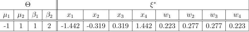
A similar result can be obtained for the corresponding maximinD-optimal three point designs in the probit model (see Table 4). Only for the parameter region Θ = [−1,1]×[1,2], three support points are not sufficient for global maximin D-optimality (see Figure 2). The corresponding maximin D-optimal four point design, which is also optimal within the class of all designs, is given in Table 5. The optimality check by the equivalence theorem for the design corresponding to the parameter region Θ = [−1,1]×[1,2] is carried out in Figure 2.
Considering the maximin D-optimal three point designs for the respective link functions, it is remarkable that the designs corresponding to the probit model allocate almost half of the weight to the support point in the center. In the logistic case, however, the situation appears to be rather different. If the maximinD-optimal two point design is already close to the maximin
Table 3: MaximinD-optimal three point designs for the logit link function with respect to various parameter spaces.
Θ ξ∗
µ1 µ2 β1 β2 x1 x2 x3 w1 w2 w3
[image:13.612.56.389.234.339.2]-1 1 23 32 -1.889 0 1.889 0.331 0.338 0.331 -1 1 1 2 -1.559 0 1.559 0.281 0.438 0.281 0 1 1 2 -0.655 0.5 1.655 0.415 0.170 0.415 -0.5 0.5 1 2 -1.155 0 1.155 0.415 0.170 0.415
Table 4: Maximin D-optimal three point designs for the probit link function with respect to various parameter spaces.
Θ ξ∗
µ1 µ2 β1 β2 x1 x2 x3 w1 w2 w3
-1 1 2 3
3
2 -1.436 0 1.436 0.262 0.476 0.262
-1 1 1 2 -1.223 0 1.223 0.255 0.490 0.255 0 1 1 2 -0.484 0.5 1.484 0.273 0.454 0.273 -0.5 0.5 1 2 -0.984 0 0.984 0.273 0.454 0.273
almost four support points are needed for maximin D-optimality, the optimal design assigns more weight to the middle point.
The final goal of this section is to investigate the performance of the maximin D-optimal designs (with respect to various parameter spaces Θ) obtained by our method, in particular the performance of the maximin D-optimal two point designs. An obvious action we can take to achieve this aim is to have a close look at the D-efficiencies of the respective designs with respect to different values of ϑ within the particular parameter space. Note that the criterion value Ψ−∞(ξ∗) of the maximin D-optimal k point design ξ∗ (where k denotes the number of
support points of ξ∗) itself represents the maximum of the minimal D-efficiencies within the corresponding class of designs. It is thus natural from the choice of our optimality criterion to start our study with the minimal D-efficiencies over the parameter space Θ of the maximinD -optimal two (and more) point designs calculated above. It is illustrated in Table 6 that (even
Table 5: Maximin D-optimal four point design for the probit link function with respect to the parameter space Θ = [−1,1]×[1,2].
Θ ξ∗
µ1 µ2 β1 β2 x1 x2 x3 x4 w1 w2 w3 w4
[image:13.612.58.470.605.659.2]Figure 2: The function d(ξ∗, x) from the equivalence theorem in the probit model. Left: The
maximinD-optimal three point design with respect to Θ = [−1,1]×[1,2](almost globallyΨ−∞
-optimal). Right: The maximin D-optimal four point design with respect to Θ = [−1,1]×[1,2]
(globally Ψ−∞-optimal).
-2 -1 1 2
1.75 1.8 1.85 1.9 1.95
2.05 -2 -1 1 2
1.65 1.7 1.75 1.8 1.85 1.9 1.95
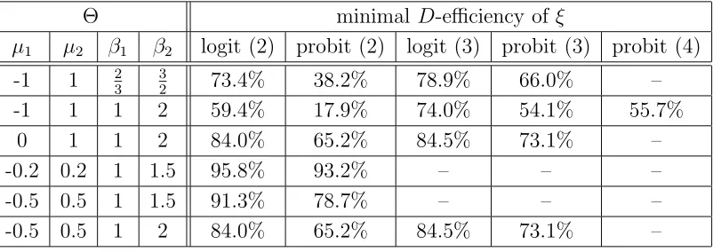
for the globally maximin D-optimal designs) the minimal D-efficiency decreases with larger parameter spaces Θ, which is intuitively clear. Moreover, the loss in D-efficiency caused by a restriction to a k point design is significantly larger in the probit model compared to the logit case, particularly if only the maximin D-optimal two point designs are considered. If, on the other hand, a third design point is added, the increase in minimal D-efficiency is remarkable in the probit model. For the logistic regression, this increase is substantially smaller.
Table 6: Minimal D-efficiencies of the maximinD-optimal k point designs ξ from the examples of Table 2 (in parentheses: the number of support points of ξ). If there is no entry in the table, the two or three-point design is already globally optimal.
Θ minimal D-efficiency of ξ
µ1 µ2 β1 β2 logit (2) probit (2) logit (3) probit (3) probit (4)
-1 1 2 3
3
2 73.4% 38.2% 78.9% 66.0% –
-1 1 1 2 59.4% 17.9% 74.0% 54.1% 55.7% 0 1 1 2 84.0% 65.2% 84.5% 73.1% – -0.2 0.2 1 1.5 95.8% 93.2% – – – -0.5 0.5 1 1.5 91.3% 78.7% – – – -0.5 0.5 1 2 84.0% 65.2% 84.5% 73.1% –
Note that the D-efficiencies from Table 6 are the minimal D-efficiencies with respect to the respective parameter regions Θ representing the worst case scenario. If the true value ofϑ ∈Θ is not an element of the supportN(ξ) of the least favourable distribution the D-efficiency of ξ
[image:14.612.60.461.403.545.2]respective designs increase rapidly if the ”true” value is someway distant from the support
[image:15.612.116.485.184.450.2]N(ξ) of the least favourable distribution, i.e. theD-efficiencies as functions ofµandβ increase steeply in a neighborhood ofN(ξ).
Figure 3: The D-efficiencies of the maximin D-optimal two point designs with respect to Θ = [−1,1]×[1,2]and the corresponding globally optimal designs. Top left: The maximinD-optimal two point design for the logistic regression model. Top right: The maximin D-optimal two point design for the probit model. Bottom left: The globally maximin D-optimal design for the logit model. Bottom right: The globally maximin D-optimal design for the probit case.
1 1.2 1.4 1.6 1.8 2 -1 -0.5 0 0.5 1 0.6 0.7 0.8 0.9 1 1 1.2 1.4 1.6 1.8 1 1.2 1.4 1.6 1.8 2 -1 -0.5 0 0.5 1 0.2 0.4 0.6 0.8 1 1 1.2 1.4 1.6 1.8 1 1.2 1.4 1.6 1.8 2 -1 -0.5 0 0.5 1 0.75 0.8 0.85 1 1.2 1.4 1.6 1.8 1 1.2 1.4 1.6 1.8 2 -1 -0.5 0 0.5 1 0.6 0.7 0.8 1 1.2 1.4 1.6 1.8
Table 7 gives the D-efficiencies of the maximin optimal designs corresponding to the situation in Figure 3 with respect to some representative ”true” values of ϑ ∈ [−1,1]×[1,2]. Since the minimal D-efficiencies (at least for two point designs) always occur on the vertices of the parameter region Θ we have already compared the D-efficiencies with respect to the vertices of Θ in Table 6. These results indicate that the maximin D-optimal designs yield reasonable
D-efficiencies over a broad range of Θ.
Table 7: Some D-efficiencies of the maximin D-optimal two point and globally maximin D -optimal designs ξ with respect to the parameter region Θ = [−1,1]×[1,2].
True ϑ D-Efficiency of ξ
µ β logit (2) probit (2) logit (global) probit (global) 0 1.5 100% 87.6% 87.2% 72.0% -0.5 1.25 90.9% 66.9% 86.7% 77.3% 0.5 1.25 90.9% 66.9% 86.7% 77.3% -0.5 1.75 89.2% 69.1% 82.7% 67.7% 0.5 1.75 89.2% 69.1% 82.7% 67.7%
reason for this observation can be found in the structure of the considered optimality criterion. The globally maximin D-optimal designs ξ protect the experiment against the worst case with respect to Θ, i.e. the true value of the parameter vector ϑ is in the setN(ξ). The optimality of
ξ on this set is ”bought” at the expense of lowerD-efficiencies with respect to parameter values in Θ\ N(ξ). Since we cannot eliminate the possibility that the ”true” parameter is a support point of the least favourable distributionπ∗,it is, relatively speaking, still recommended to use
the globally maximin D-optimal designs ξ when Θ is large, because optimal designs with re-spect to this criterion yield some protection against the worst case scenario, which the maximin
D-optimal two point designs cannot accomplish for large parameter regions Θ.
In the following, we consider another somewhat related indicator for the performance of a design
ξ with a restricted number of support points, i.e. its efficiency with respect to the criterion function Ψ−∞,
effΨ−∞(ξ) =
Ψ−∞(ξ)
maxηΨ−∞(η)
,
where the maximum is taken over the set of all designs. For the maximin D-optimal two point designs Ψ−∞-efficiencies are listed in Table 8.
Table 8: Ψ−∞-efficiencies of the MaximinD-optimal two point designsξ, which are not globally
optimal.
Θ effΨ−∞(ξ)
µ1 µ2 β1 β2 logit probit
-1 1 2 3
3
2 92.9% 57.9%
[image:16.612.55.251.527.635.2]For the logistic regression model the efficiencies taken from Table 8 are quite high, so that for moderate regions Θ it seems sufficient to use the corresponding maximin D-optimal two point design provided that the data should not be used for a goodness-of-fit test of the model. However, the use of the maximin D-optimal two point design in the probit model can only be recommended for small parameter spaces. As pointed out before, the implementation of our method is much easier if only two point designs are required. Furthermore, it may reduce costs for the experimenter, if the number of support points is as low as possible. If, on the other hand, the parameter space specified by the experimenter is larger, it is recommended to use the modified algorithm and calculate the globally maximin D-optimal design [see Section 3]. Another situation, in which the determination of maximin D-optimal designs with more than two support points is necessary, occurs if the design should also be used for model checking.
5
Appendix: Proofs
Proof of Theorem 1: The first part is a special case of Theorem 2.1 from Dette, Haines and Imhof (2004) where the criterion function ψ(M(ξ, ϑ)) is given by the (square root of the) determinant of the Fisher information, which is obviously continuous in each argument. Let the sequence of prior distributions {πq}q≤0 be constant in q, i.e. πq =π for all q ≤ 0 and
let supp(π)=E. The proof of the second part then follows along the same lines as the proof of the above-mentioned theorem where the parameterθ is chosen from E instead of Θ. If the set E is discrete it is not necessary (and possible) to define open neighborhoods within the set E around the elements θE ∈ E. Instead of its neighborhood the respective θE itself can
be inserted in the proof of Theorem 2.1 from Dette, Haines and Imhof (2004) since π(θE)>0
holds for each element of E. 2
Proof of Theorem 3: In the first step of this proof, we will show that the gradient of the function log|M(ξ, ϑ)| with respect to the parameters has at most one root, and exactly one root if the functionh(z) features a local extremum. Note that all of the commonly applied link functions have this property. Let h(z) be strictly log-concave. Using the formula
|M(ξ, ϑ)|= 1
4h(β(x1−µ))h(β(x2−µ))(x2−x1)
2β2
for the determinant of the information matrixM(ξ, ϑ) of a two point designξwith equal weights at the support pointsx1, x2 we obtain the gradient of log|M(ξ, ϑ)| as
∂log|M(ξ, ϑ)|
∂ µ = −β h0
h|β(x1−µ)−β
h0
h|β(x2−µ)
(A.1)
∂log|M(ξ, ϑ)|
∂ β =
2
β + (x1−µ) h0
h|β(x1−µ)+ (x2−µ)
h0
h|β(x2−µ)
where h0
h|z denotes the first derivative of loghevaluated at a pointz. Replacingβ(xi−µ) byγi
and setting the gradient (A.1) equal to zero, we get the following system of nonlinear equations.
h0 h|γ1 +
h0
(A.2)
γ1
h0
h|γ1 +γ2
h0
h|γ2 + 2 = 0
We now consider the first equation in (A.2). Without loss of generality we assume that γ1 > γ2.
If h features no local extremum, i.e. h0 has no root, the first equation will have no solution at all due to the continuity of the first derivative h0
h and the fact that h0
h is strictly monotonic
decreasing since logh is concave. In this case, the gradient has no roots, so log|M(ξ, ϑ)| is strictly unimodal with respect to the parameters. If, however, there is a point γ0 with
h0(γ
0) = 0, which is true for all the commonly applied link functions, the continuity and strict
monotonicity of hh0 imply that there exist values ofγ1 > γ0 such that there is a unique solution
γ2 =γ2(γ1) of the first equation in (A.2). We define the supremum of these values as ¯γ. (There
might be values of γ1 such that there is no appropriate γ2.) For any γ1 ∈ (γ0,¯γ) we now use
γ1, γ2(γ1) in the second equation of (A.2). The goal is to show that there is exactly one γ1∗
such that (γ1∗, γ2∗) = (γ1∗, γ2(γ1∗)) is the unique solution of the second equation. From (A.2), we
obtain
(γ1−γ2(γ1))
h0
h|γ1 =−2
(A.3)
and define the left hand side as functionk(γ1) = (γ1−γ2(γ1))h
0
h|γ1. Obviously, we havek(γ0) = 0
and limγ1→¯γk(γ1) = −∞, since h0
h|γ1 < 0 ∀ γ1 > γ0 and limγ1→¯γ(γ1 −γ2(γ1)) = ∞. (Either
¯
γ = ∞ or if ¯γ < ∞ then limγ1→γ¯γ2(γ1) = −∞.) It remains to show that k(γ1) is strictly
decreasing, which implies that there is exactly one tupel (γ∗
1, γ2(γ1∗)), which solves (A.2). The
derivative ofk(γ1) is given by
k0(γ1) =
h0 h 0 γ1
(γ1−γ2(γ1)) +
h0
h|γ1(1−γ
0
2(γ1)).
(A.4)
The term h0
h 0
γ1
is less than zero for all γ1 ∈ (γ0,γ¯) since this is the second derivative of
logh(γ1), which is negative due to the log-concavity of h. The term (γ1−γ2(γ1)) is positive
because we assumed that γ1 > γ2, which makes the first addend in (A.3) negative. As γ1 > γ0
we have hh0|γ1 <0. The application of the Implicit Function Theorem to the function h0
h|γ1+ h0
h|γ2,
finally, yields that γ20(γ1)<0 for all γ1 ∈(γ0,¯γ), i.e. 1−γ20(γ1) >0. The derivative ofk with
respect to γ1 is therefore negative for all γ1 ∈ (γ0,γ¯). So k is strictly decreasing from zero to
−∞. It follows that there is exactly one γ∗
1, for which k(γ∗1) = −2 and therefore the solution
of (A.2) exists and is unique.
As the mapping (γ1, γ2) = (β(x1−µ), β(x2−µ)) for fixed x1, x2 is one-to-one, the root of
the gradient is also unique in terms ofβ and µ.
In the following step, we will show that the function log|M(ξ, ϑ)|attains its local (and global) maximum at the unique root of its gradient. Let, for the sake of typographical brevity, δ(x) denote the second derivative of log h(z) evaluated at the pointz =β(x−µ).
We calculate the eigenvalues of the Hessian H of log|M(ξ, ϑ)| with respect toµ and β as
λ1,2 =
H11+H22
2 ±
r
(H11+H22)2
4 −H11H22+H
where Hij, i, j= 1,2,denote the entries of H. Since
H11 = β2δ(x1) +β2δ(x2), H22 = −
2
β2 + (x1−µ) 2δ(x
1) + (x2−µ)2δ(x2),
H12 = −
h0
h|β(x1−µ)−β(x1−µ)δ(x1)−
h0
h|β(x2−µ)−β(x2−µ)δ(x2)
we see immediately that the smaller eigenvalue is less than zero if δ(x) <0 for all x ∈IR, i.e.
h(z) log-concave in z ∈IR. The product of the eigenvalues λ1λ2 turns out to be
λ1λ2 = −2(δ(x1) +δ(x2)) +β2δ(x1)δ(x2)(x2−x1)2
(A.5)
− h 0
h|γ1 +
h0
h|γ2 2
−2βh
0
h|γ1 +
h0
h|γ2
((x1−µ)δ(x1) + (x2−µ)δ(x2))
which is positive at the point (γ1∗, γ2∗) if, again, δ(x) < 0 for all x ∈ IR since the second line
of (A.5) vanishes as the term h0
h|γ1∗ + h0
h|γ2∗
is equal to zero. Hence the larger eigenvalue is also negative at the point (γ∗1, γ2∗) and therefore log|M(ξ, ϑ)| attains a local maximum at the unique root of its gradient with respect toµ and β. Since the gradient has only one root, the
maximum is also global. 2
Proof of Theorem 4: For the sake of typographical brevity, we define the D-efficiency Φ(ξ, ϑ) := (|M(ξ, ϑ)|/|M(ξϑ, ϑ)|)1/2. As a first step in the proof, we show that for every equally
weighted two point designξ the function|M(ξ, ϑ)|and thus the square root of the standardized version Φ(ξ, ϑ) is log-concave with respect to the design points x1, x2 for all ϑ ∈ Θ if h(z) is
log-concave and twice differentiable. (Note that the maximinD-optimal two point design must have equal weights [see Silvey (1980)].) We calculate the eigenvaluesλx1,2 of the Hessian Hx of
log|M(ξ, ϑ)| with respect to x1 and x2 as
λx1,2 =
Hx11+Hx22
2 ±
r
(Hx11+Hx22)2
4 −Hx11Hx22+H
2
x12,
whereHxij, i, j = 1,2, denote the entries ofHx. Since
Hx11 = β2δ(x1)−
2 (x1−x2)2
, Hx22 = β2δ(x2)−
2 (x1−x2)2
,
Hx12 =
2 (x1−x2)2
and δ(x) < 0 for all x, the smaller eigenvalue is obviously negative. The product of the eigenvalues, however, is given by
β4δ(x1)δ(x2)−β2δ(x1)
2
(x1−x2)2 −
β2δ(x2)
which is positive for all choices of x1 and x2. The larger eigenvalue is therefore also negative
and the function Φ(ξ, ϑ) is log-concave.
In the second step of the proof we will show that log-concavity of Φ(ξ, ϑ) with respect to x1
andx2 implies the uniqueness of the maximinD-optimal two point design. Define two different
designs ξ(1), ξ(2) with support points x(1)
i , x
(2)
i , i = 1,2, respectively, and construct a further
designξ(1,2) by x(1,2)
i = (x
(1)
i +x
(2)
i )/2, i= 1,2. For fixed values of ϑ we have
Φ(ξ(1,2), ϑ)>min{Φ(ξ(1), ϑ),Φ(ξ(2), ϑ)} (A.6)
because of the log-concavity of Φ(ξ, ϑ) in x1, x2. Let nowξ(1), ξ(2) be two maximin D-optimal
two point designs with optimal criterion value Ψ∗−∞, i.e. minϑ∈ΘΦ(ξ(1), ϑ) = minϑ∈ΘΦ(ξ(2), ϑ) =
Ψ∗
−∞.In particular, we have
Φ(ξ(1), ϑ)≥Ψ∗−∞, Φ(ξ(2), ϑ)≥Ψ∗−∞ ∀ϑ∈Θ.
(A.7)
The above minima exist because Θ is assumed to be compact, which also implies that the set
N(ξ(1,2)) is not empty. From the optimality of the value Ψ∗
−∞ we obtain for all ϑ∗ ∈ N(ξ(1,2))
the inequality Φ(ξ(1,2), ϑ∗)≤Ψ∗
−∞. But from (A.6) and (A.7) it follows that
Φ(ξ(1,2), ϑ∗)>min{Φ(ξ(1), ϑ∗),Φ(ξ(2), ϑ∗)} ≥Ψ∗−∞,
which is a contradiction to the assumption that there exist more than one Ψ−∞-optimal two
point design. 2
Proof of Lemma 5. Since the value of the determinant of the locally D-optimal design
|M(ξϑ, ϑ)|does not depend onϑ∈ Θ,the standardized maximinD-optimal design with respect
to ˜Θ = [µ1+∆
c ,
µ2+∆
c ]×[cβ1, cβ2] can be obtained by maximizing
min
β∈[cβ1,cβ2] µ∈[µ1+∆c ,µ2+∆c ]
Z
h(β(x−µ)) β
2 −β(x−µ)
−β(x−µ) (x−µ)2 )dξ(x)
= min
β∈[β1,β2] µ∈[µ1,µ2]
Z
h(cβ(x− µ+ ∆
c ))
c2β2 −cβ(x− µ+∆
c )
−cβ(x− µ+∆c ) (x− µ+∆
c )2
dξ(x)
= min
β∈[β1,β2] µ∈[µ1,µ2]
Z
h(β(x−µ)) c
2β2 −β(x−µ)
−β(x−µ) 1
c2(x−µ)2
dξ˜(x)
where the design ˜ξ is obtained fromξ by the relation ˜
ξ({x}) =ξ({cx−∆}).
The assertion of Lemma 5 is now obvious. 2
References
[1] Abdelbasit, K.M. and Plackett, R.L. (1983). Experimental design for binary data.Journal of the American Statistical Association, 78, 90-98.
[2] Chaloner, K. and Larntz, K. (1989). Optimal Bayesian experimental design applied to logistic regression.Journal of Statistical Planning and Inference, 21, 191-208.
[3] Chernoff, H. (1953). Locally optimal designs for estimating parameters. Annals of Mathe-matical Statistics, 24, 586-602.
[4] Dette, H. (1997). Designing experiments with respect to standardized optimality criteria.
Journal of the Royal Statistical Society, Ser. B, 59, No.1, 97-110.
[5] Dette, H., Haines, L. and Imhof, L. (2003). Maximin and Bayesian optimal designs for regression models. Under revision for: Annals of Statistics.
http://www.ruhr-uni-bochum.de/mathematik3/preprint.htm
[6] Dette, H., Haines, L. and Imhof, L. (2004). Maximin and Bayesian optimal designs for heteroscedastic regression models. Under revision for: Canadian Journal of Statistics. http://www.ruhr-uni-bochum.de/mathematik3/preprint.htm
[7] Dette, H. and Wong, W.K. (1996). Optimal Bayesian designs for models with partially specified heteroscedastic structure. Annals of Statistics, 24, No. 5, 2108-2127.
[8] Fandom Noubiap, R. and Seidel, W. (2000). A minimax algorithm for constructing optimal symmetrical balanced designs for a logistic regression model.Journal of Statistical Planning and Inference, 91, No. 1, 151-168.
[9] Ford, I., Torsney, B. and Wu, C.F.J. (1992). The use of a canonical form in the construction of locally optimal designs for non-linear problems.Journal of the Royal Statistical Society, 54, 569-583.
[10] Imhof, L. (2001). Maximin designs for exponential growth models and heteroscedastic polynomial models.Annals of Statistics, 29, No. 2, 561-576.
[11] Kalish, L.A. and Rosenberger, J.L. (1978). Optimal designs for the estimation of the logistic function.Technical Report 33, Department of Statistics, Pennsylvania State University.
[12] Minkin, S. (1987). Optimal designs for binary data. Journal of the American Statistical Association, 82, 1098-1103.
[13] M¨uller, C. H. (1995). Maximin efficient designs for estimating nonlinear aspects in linear models. Journal of Statistical Planning and Inference, 44, 117-132.
[14] Silvey, S.D. (1980).Optimal Design. Chapman and Hall, London.
[16] Sitter, R.R. and Fainaru, I. (1997). Optimal designs for the logit and probit models for binary data. Canadian Journal of Statistics, 25, No. 2, 175-190.
[17] Sitter, R.R. and Wu, C.F.J. (1993). Optimal designs for binary response experiments: Fieller-, D- and A-criteria. Scandinavian Journal of Statistics, 20, 329-341.
[18] Wu, C.F.J. (1988). Optimal design for percentile estimation of a quantal response curve.

![Table 7: Someoptimal designs D-efficiencies of the maximin D-optimal two point and globally maximin D- ξ with respect to the parameter region Θ = [−1, 1] × [1, 2].](https://thumb-us.123doks.com/thumbv2/123dok_us/8507956.349279/16.612.55.251.527.635/someoptimal-designs-eciencies-maximin-optimal-globally-maximin-parameter.webp)
