Habitat association, disturbance dynamics, and the role of spatial scale in structuring coral reef fish assemblages
218
0
0
Full text
(2) Habitat association, disturbance dynamics, and the role of spatial scale in structuring coral reef fish assemblages. Thesis submitted by Craig SYMS BSc Canterbury MSc (Hons) Auckland in March 1998. for the degree of Doctor of Philosophy in the Department of Marine Biology James Cook University of North Queensland.
(3) STATEMENT OF ACCESS. I, the undersigned, the author of this thesis, understand that James cook University of North Queensland will make it available for use within the University Library and, by microfilm or other means, allow access to users in other approved libraries. All users consulting this thesis will have to sign the following statement: In consulting this thesis I agree not to copy or closely paraphrase it in whole or part without the written consent of the author; and to make proper public written acknowledgement for any assistance that I have obtained from it. Beyond this I do not wish to place any restrictions on access to this thesis.. t49.
(4) Abstract. Understanding how patterns and processes at one scale are related to those at other scales is of central importance in developing ecological theory. However, in order for scaling rules to be useful to empirical ecologists, they must have a rational, measurable, and critically examinable basis. In this study I consider the role spatial scale plays in structuring coral reef fish assemblages and how habitat structure may mediate scaling rules for the assemblage. The relationship between a population's mean and variance provide a measure of whether that population is indeed scale dependent. I counted fish and measured habitat variables in 701 transects, allocated across 12 habitat zones. Slopes of the power plots for most species lay between 1 and 2 which indicated that the variance, as a proportion of the mean, of small samples was lower than in large samples and hence scaledependent. 28% of the variation of the data set was explained by habitat variables which indicated that a large percentage of the scale dependence could be modelled by habitat variables alone. Peaks of variability associated with changes in scale are indicators of the scales at which organisms are spatially structured. It has been hypothesised that coincident variance peaks are indicators of common scales of organisation and thus should also correspond to the scale of maximal correlation. I tested this idea by quantifying fishhabitat associations at different scales on contiguous coral reefs. I mapped fish and habitat to a 3x3m resolution in 24 30x30m grids and then progressively aggregated adjacent squares and recalculated the correlation between fish and benthic cover, physical reef structure, and locality over 9 spatial scales ranging from 9-225m2 . Both fish and habitat variables were patchy at the smallest scale, yet maximal correlation occurred at larger scales (>54m 2). A complex suite of responses were found among fish taxa, with some species associated simply with'benthic cover and locality, while others were associated with complex interactions between different types of habitat measures. The scale of maximal correlation was not indicative of the scale at which fishes responded to their environment. Maximal correlation was found when the likelihood of the occurrence of a particular fish species and the likelihood of the occurrence of.
(5) -11-. preferred habitat type were symmetrised. In other words, the scale of measurable fishhabitat association was a measurement of the optimal scale at which predictability of fish given habitat type, and predictability of habitat type given fish were maximised. Studies carried out on small patch reefs have provided the basic information from which much ecological theory of coral reef fishes has been derived. However no published studies have attempted to document what scaling effects exist in coral reef systems, and whether we can extrapolate or interpolate between studies carried out on different scales. I mapped randomly selected patch reefs, ranging in size from 0.26m 2 to 63.5m2, and censused the resident fish fauna. I then partitioned variation amongst reef area, reef shape and patchiness, and benthic cover. Species responded in a variety of ways to reef parameters. Some species were strongly area-dependent, others were well predicted by reef shape and patchiness, and a considerable number of species were well predicted by the benthic cover of the reef. Further groups of species were associated with combinations of these factors. In order to measure the effect of scaling up or down, I divided the data set into small, medium, and large reefs, recalculated regression equations and measured the predictive ability of each equation. Surprisingly equations derived from the smaller reefs were better predictors of larger reefs than vice versa. As a consequence, the lessons drawn from experiments carried out on small reefs can, in the light of prior information, be cautiously, and with strong caveats, applied to large reefs. Central to these scaling rules is the incorporation of habitat as an explanatory variable. To establish the bounds within which habitat may influence fish assemblage structure, I carried out two experiments. First, I experimentally reduced coral cover in 10x10m quadrats on contiguous reef from 55% to 47%, 43%, and 34% and monitored the assemblage over two years. Contrary to what might be expected from many correlative studies, all fish species considered were resistant, at this scale and level, to habitat disturbance. However, a large portion of variation in the fish assemblage was explainable by spatial and temporal variables. It is hypothesised that spatial-temporal structure at the landscape level may moderate local disturbance to habitat structure on contiguous reef. The second disturbance experiment was carried out on small patch reefs. To reevaluate the current models of reef fish assemblage organisation, I implemented a factorial combination of direct (by fish removal) and indirect disturbance (by habitat alteration) and monitored the experiment over two years. Habitat disturbance generated.
(6) strong, predictable changes in the fish assemblage which explained almost half the variation in the data set. In contrast, direct disturbance generated a lesser and shorterterm effect. The results from this experiment supported a model of reef fish assemblages as deterministic (within broad bounds), yet weakly interacting systems, the determinism of which was mediated by habitat. This study supports the initial premise that scaling rules for coral reef fish assemblages are mediated by habitat. As a consequence, habitat structure must be included into a general theory of coral reef fish ecology. An important precursor to the successful incorporation will be the parameterisation of the spatio-temporal dynamics of habitat structure, and the scales and forms of responses to habitat disturbance that fishes can be expected to make. Scale, far from being a black-box within which incongruous results are filed, can exert rational, mechanistic effects which can be incorporated both into the theoretical and empirical development of coral reef fish ecology..
(7) -iv-. Acknowledgements. I would like to thank my supervisor, Dr Geoff Jones, for granting me free rein to pursue the lines of inquiry that took my fancy, and furthermore picking up the tab courtesy of his Australian Research Council grant. I thank Geoff also for his many conversations, ideas, and criticisms that have served to focus my research over the years. The Australian Museum's Lizard Island Research Station provided the logistical support without which I could not have spent the many diving hours required to address the questions that I found interesting. Many thanks to the directors, Anne Hoggett and Lyle Vail, and support staff, Lance and Marianne. I thank also the numerous and varied diving assistants who bore with me, wondering how it was possible to look at the same piece of rock for 30 minutes and still retain enough enthusiasm to relish the thought of looking at another rock for a further half hour ad infinitum. Extra special thanks to Tara Anderson for her patch-reef map drawing and image analysis skills; her copious proof reading; graphical and word processing expertise; long discussions about what's wrong with science (we can't be wrong, can we?); her tireless perfectionism during the latter stages of this thesis - long after I ceased to care what it looked like; and her perennial love and support..
(8) -v-. STATEMENT ON SOURCES DECLARATION. I declare that this thesis is my own work and has not been submitted in any form for another degree or diploma at any university or other institute of tertiary education. Information derived from the published or unpublished work of others has been acknowledged in the text and a list of references is given.. 1. 0C-r. 199 S.
(9) -vi-. Table of Contents. Abstract iv. Acknowledgements Signed Statement of Sources. vi. Table of Contents List of Tables. viii. List of Figures. Chapter I: General Introduction 1.1 Overview. 1. 1.2 Reef fish ecology, scale, habitat, and disturbance. 1. 1.3 Thesis outline. 3. Chapter 2: Habitat Heterogeneity Mediates the Scaling of a Reef Fish Assemblage 2.1. Abstract. 5. 2.2. Introduction. 5. 2.3. Methods. 8. 2.4. Results. 9. 2.5. Discussion. 18. Chapter 3: At What Scales are Fish Associated with their Habitat? An Empirical Study 3.1. Abstract. 21. 3.2. Introduction. 21. 3.3. Methods. 24. 3.4. Results. 26. 3.5. Discussion. 47.
(10) -viiChapter 4: Scaling Rules and Patch Reefs: Are Large Patches Simply Collections of Small Patches? 4.1. Abstract. 54. 4.2 Introduction. 54. 4.3 Methods. 57. 4.4 Results. 61. 4.5 Discussion. 79. Chapter 5: Disturbance and the Structure of Coral Reef Fish Communities on the Reef Slope 5.1 Abstract. 82. 5.2 Introduction. 82. 5.3 Methods. 84. 5.4 Results. 88. 5.5 Discussion. 99. Chapter 6: The Structure of Coral Reef Fish Communities: Direct versus Indirect Effects of Disturbance 6.1 Abstract. 103. 6.2 Introduction. 104. 6.3 Methods. 108. 6.4 Results. 111. 6.5 Discussion. 130. Chapter 7: General Discussion. 136. References. 142. Appendix I.. 157. Appendix II.. 168. Appendix DI. 182.
(11) List of Tables. Chapter 2: Habitat Heterogeneity Mediates the Scaling of a Reef Fish Assemblage 2.1 Habitat classes and sample allocation. 12. 2.2 Analysis of variance of species richness per transect. 13. Chapter 3: At What Scales are Fish Associated with their Habitat? An Empirical Study 3.1. Correlations between pomacentrids and habitat variables. 34. 3.2. Correlations between labrids and habitat variables. 35. 3.3. Correlations between chaetodontids and habitat variables. 36. 3.4. Correlations between pomacanthids and habitat variables. 36. Chapter 4: Scaling Rules and Patch Reefs: Are Large Patches Simply Collections of Small Patches? 4.1. Correlation of reef parameters with principal components.. 67. 4.2. Correlation of benthic cover with principal components. 67. 4.3. Number of species in each family. 68. 4.4. Multiple regression of species richness with patch reef parameters. 69. 4.5. Multiple regression parameters of species with reef parameters. 70. Chapter 5: Disturbance and the Structure of Coral Reef Fish Communities on the Reef Slope 5.1 Decomposition of variation to different fractions. 90. 5.2 Pre-existing associations between fish, benthic cover, and assignment of quadrats to treatments. 91. 5.3 Importance of factors relative to total variation explained by CDA. 92.
(12) Chapter 6: The Structure of Coral Reef Fish Communities: Direct versus Indirect Effects of Disturbance. 6.1 MANOVA of the first 20 principal components of the covariance matrix. 115. 6.2 Structure coefficients of species in the CDA of temporal changes in adults. 116. 6.3 MANOVA of total recruits per reef. 117. 6.4 Characteristic features of species responses to different disturbances derived from raw data. 118.
(13) -x-. List of Figures. Chapter 2: Habitat Heterogeneity Mediates the Scaling of a Reef Fish Assemblage 2.1 Species abundance distributions of pomacentrids.. 14. 2.2 Distribution of slope parameters from power-plots of 55 pomacentrid species. 15. 2.3 Percent variance of the pomacentrid assemblage explained by benthic cover, habitat class and their interaction. 16. 2.4 Canonical Correspondence Analysis of pomacentrids with habitat class and benthic cover. 17. Chapter 3: At What Scales are Fish Associated with their Habitat? An Empirical Study 3.1 Location of sample grids around Lizard Island. 37. 3.2 Average depth and topography for each locality. 38. 3.3 Variance of depth and topgraphy with changing scale. 39. 3.4 PCA biplot of benthic cover of each site. 40. 3.5 Proportional variance profiles of benthic cover. 41. 3.6 Proportional variance profiles of pomacentrids, labrids, chaetodontids, and pomacanthids. 42. 3.7 Changes in variance explained by different sets of habitat variables for pomacentrids. 43. 3.8 Changes in variance explained by different sets of habitat variables for labrids. 44. 3.9 Changes in variance explained by different sets of habitat variables for chaetodontids. 45. 3.10 Changes in variance explained by different sets of habitat variables for pomacanthids. 46. Chapter 4: Scaling Rules and Patch Reefs: Are Large Patches Simply Collections of Small Patches? 4.1 Maximum length and width of patch reefs examined.. 71. 4.2 Correlations between reef patchiness parameters.. 72.
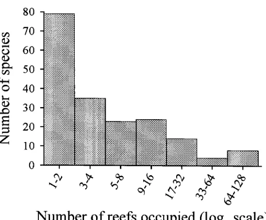
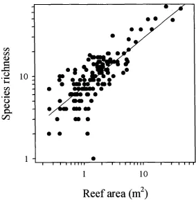
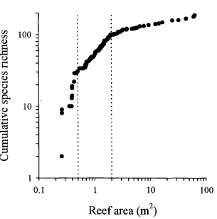
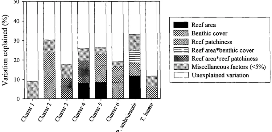
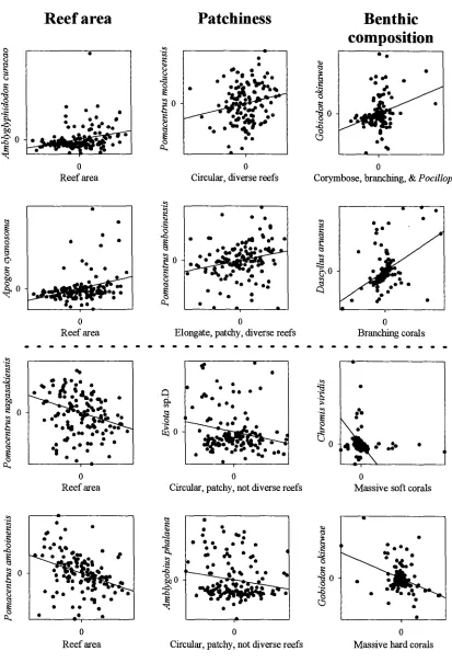
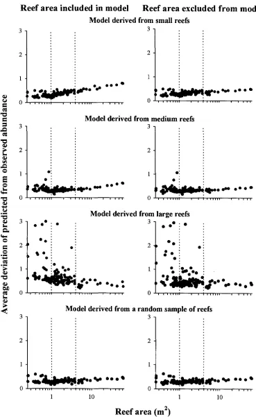
(14) -xi4.3. Number of reefs occupied by different species. 73. 4.4. Relationship between species richness and patch reef area. 74. 4.5. Cumulative species richness vs ranked reef area.. 75. 4.6. Percent variance explained by reef area, benthic cover, reef patchiness, and their interaction effects.. 76. 4.7. Partial regression plots of selected fish-habitat relationships. 77. 4.8. Predictive ability of small, medium, large, and a random sub sample of reefs. 78. Chapter 5: Disturbance and the Structure of Coral Reef Fish Communities on the Reef Slope 5.1 Location of study site at Lizard Island northern Great Barrier Reef. 93. 5.2 PCA of the correlation matrix of benthic cover in quadrats prior to manipulation. 94. 5.3 Coral reductions in experimental quadrats expressed as proportions of total hard coral cover and table/corymbose forms only 95 5.4 Percent variance explained by treatment, temporal, spatial, and interaction effects for 4 fish families 96 5.5 Abundances of a selection of positively coral-associated fish species through time 97 5.6 Abundances of a selection of negatively coral-associated fish species through time 98. Chapter 6: The Structure of Coral Reef Fish Communities: Direct versus Indirect Effects of Disturbance 6.1 Models predicting the responses of stable communities to direct, indirect and a combination of direct and indirect disturbances.. 119. 6.2 Schematic representation of the experimental design. 120. 6.3 The benthic cover of the major substratum categories on experimental patch reefs before, 3 months after and 12 months after habitat damage. 121. 6.4 The mean change in the height of experimental patch reefs before, 3 months after and 12 months after habitat damage. 122. 6.5 Temporal changes in composition and abundance across the experiment. 123. 6.6 CDA of recruit abundance pooled across the experiment. 124.
(15) 6.7 Mean recruit abundance pooled across the duration of the experiment. 125. 6.8 Patterns of change in the abundance of two abundant live coral associated species Pomacentrus moluccensis and Dascyllus reticulatus, in response to direct and indirect disturbance. 126. 6.9 Patterns of change in the abundance of two abundant species associated with dead coral substrata (P. amboinensis and P. nagasakiensis), in response to direct and indirect disturbance. 127. 6.10 Patterns of change in the abundance of two abundant rubbleassociated species (Parapercis spp. and Dischistodus perspicillatus), in response to direct and indirect disturbance. 128. 6.11 Patterns of change in mean species richness in response to direct and indirect disturbance. 129.
(16) Chapter One -1-. General Introduction. 1.1 Overview The study of reef fish ecology is a challenging and rewarding pursuit. The researcher works in an alien environment in which the familiar scales of reference no longer appear to apply. Reef fish for the most part have a bipartite life cycle in which the scales of larval dispersion appears to bear no resemblance to the scales at which the adult fish feed, mate, and otherwise carry out their existence. In addition, the researcher has a limited view of the fish community, limited by the water visibility, swimming ability, and logistical constraints. Disparities between the intuitive scale of the researcher, and the organisms they study present many problems in the study of reef fish ecology. This thesis considers the role spatial scale plays in the ecology of coral reef fishes and aims to further the development of guidelines or 'rules' that enable studies conducted at one scale to be reconciled with those conducted at others. Coral reef fish are intimately associated with their habitat, and it is my contention that habitat structure mediates much of the scale effects that have been previously observed in coral reef fish assemblages. Furthermore, I put forward that understanding the relationships and scales at which fish are associated with different elements of their habitat will enable development of an empirical framework within which we can view scaling.. 1.2 Reef fish ecology, scale, habitat, and disturbance Despite a myriad of studies (see reviews by Ehrlich 1975, Goldman and Talbot 1976, Sale 1980b, 1991a, Doherty and Williams 1988b), a general theory of reef fish ecology has not been forthcoming. This has been, at least in part, due to a shift in emphasis from 'explainable' patterns (e.g. Smith and Tyler 1972, Sale 1974, Jones 1986, 1987 a, b, Wellington 1992) to the inherently unexplainable stochasticity that forms such a significant part of the population structure of coral reef fishes (e.g. Sale 1977, 1978, 1988, Doherty 1987, Doherty and Williams 1988 a, b). It is probably unreasonable to expect that coral reef fish assemblages are so tightly organised as to be completely predictable, and indeed it may be unreasonable that we can account for even half of the variation in population or assemblage structure. However, enough studies have shown that, at some scales and within some broad context, fishes are organised enough so that.
(17) Chapter One -2pattern emerges above the surrounding noise. A more insidious trend has been for irreconcilable results to be allocated to the catch-all black box of 'scale' (Sale 1988) and, because little is known about how exactly scale operates to generate these differences, this has become sufficient explanation to explain disparities (but see Aronson 1994). In order for scale to be an acceptable explanation for an observable phenomenon, it should have a rational mechanism, and be empirically useful - i.e. a `science of scale' (Meentemeyer and Box 1987). A major ecological factor in reef fish assemblages is the habitat within which they exist, and few people would doubt that reef fish are associated with reef characters at some level (Sale 1988). It has been the experience of terrestrial landscape ecologists that understanding spatial habitat structure is the key to understanding the ecology of habitat-associates (e.g. Addicott et al. 1987, Clark 1991, Bell et al. 1995, Hanski et al. 1995, Kareiva and Wennergren 1995, Collins and Barrett 1997). It is one of the contentions in this thesis that this is no less true for coral reef fish assemblages. Unfortunately, the extensive methodologies and frameworks developed by landscape ecologists are not easily applied to reef fish assemblages (pers. obs.), and generally do not provide explanatory power at the scales at which reef fish ecologists perceive and quantify their study system (pers. obs.). The measurement of habitat and, in particular, what fishes respond to is not a trivial matter. Benthic cover, topography, depth, and locality all interact to generate a habitat that cannot be simply seen as a collection of independent factors, but as a complex suite of interacting (and often confounded) elements each conditional on the others. Despite the problems associated with quantifying habitat (Jones and Syms in press, Appendix 3), effective isolation of different habitat components is required to ascertain exactly what fishes respond to. Given the premise that habitat is central to developing scaling rules, habitat measurement must form an important part of any scaling study. In order to ascertain the importance of habitat, it is necessary to identify the boundaries within which habitat operates to regulate fish assemblages. Coral reefs are disturbed habitats (Williams 1986, Done 1992) and so natural variation due to habitat disturbance is likely to exert an effect on fish assemblages. If habitat is indeed a key to formulating scaling rules, then the dynamics of fish assemblages in response to habitat changes must be established..
(18) Chapter One -31.3 Thesis outline This thesis is a collection of five independent investigations, presented in logical rather than chronological order, into the role of scale and habitat association, and the effects of disturbance on reef fish assemblages. Although it has been frequently assumed that scale is important in reef fish ecology, few researchers have actually set out to test this assertion. In Chapter 2 I set the scene for the remainder of the thesis by using the spatial variance-mean relationship to establish that fish populations are indeed scale-dependent. I then consider the differing models, developed from terrestrial systems, that explain the power relationship and put forward the hypothesis that habitat structure plays a large role in generating the scale relationship. In addition, the question of - 'What defines a habitat?' is raised. In order to measure the scale at which organisms are associated with their habitat, it is necessary to alter the scales at which measurements are made, and re-evaluate their relationship. In Chapter 3 I present associations between fish and benthic structure, physical reef-structure, and locality, at 9 scales ranging from 9m 2 to 225m2 . I then compare the scales of patchiness of the fish and habitat, with the scales at which associations are strongest. Much of the current theory of how coral reef fish assemblages are organised was, and continues to be, developed from studies conducted on small patch reefs. Indeed, it was the apparent irreconcilability of studies carried out on different-sized reefs that first spawned the idea that scale was having a profound influence on the progress of fish ecology. In Chapter 4 I measure fish-habitat associations on patch reefs ranging from 0.26-63.5m2 in order to identify the nature of the perceived scale dependence. I then establish the context within which experiments conducted at single scales can be reconciled with the sample 'universe' of patch reefs and evaluate the ability of small, medium, and large reefs to predict assemblages on reefs of different sizes. Having established that habitat is of importance to coral reef fishes, it follows that disturbance to habitat may be a critical process regulating fish assemblage structure. In Chapter 5 I experimentally disturb hard corals on contiguous reef, and measure the response of the fish assemblage over two years. Experiments conducted on contiguous reef in permanent quadrats require particular care with regard to spatial and temporal autocorrelation, and the analytical safeguards I employ to account for these factors in themselves yield insight into the organisation of contiguous-reef assemblages..
(19) Chapter One -4Having considered the effect of physical disturbance on contiguous reef, it follows that similar disturbances may be important on patch reefs. In Chapter 6 I compare the relative effects of direct disturbance (by fish removal) versus indirect disturbance (by habitat alteration) on patch-reef fish assemblages. Furthermore, I develop a model of reef fish as weakly interacting, yet deterministic (albeit variable) assemblages. Finally, in the General Discussion I summarise the premise of this thesis that scale effects occur, and may be understood by reference to the habitat. I conclude by highlighting future directions that I believe will further centralise a theory of reef fish ecology..
(20) Chapter Two -5-. Chapter Two: Habitat Heterogeneity Mediates the Scaling of a Reef Fish Assemblage. 2.1 Abstract. Scale has been invoked as a phenomenon that explains a wide range of divergent observations in different studies. However, few studies have actually addressed whether scale-dependence is in fact present and hence a possible explanation for differences in results. I considered whether damselfish populations are spatially scaledependent and if so, what mechanism was likely to be responsible for generating scale dependence. I measured the log(variance)/log(mean) relationship for 65 species of damselfish in 701 transects around Lizard Island on the northern Great Barrier Reef, Australia. Slopes of the power plots generally fell between 1-2 and differed between species, but within a species did not differ between habitats. Two hypotheses have been put forward to explain the variance-mean relationship. First is a hypothesis based on species-specific behavioural aggregation; the second is based on environmental heterogeneity. The results of this study shared elements of both the behavioural and habitat-heterogeneity hypotheses. However, the habitat association observed in this study, in combination with prior knowledge about reef fish ecology and behaviour, would support a hybrid model in which environmental heterogeneity mediated much of the scale-dependence of reef fish, but species-specific idiosyncracies exert a stabilizing influence at the smaller scale. These results suggest that pomacentrid populations are scale dependent, and that habitat structure is an important covariate of this scale-dependence. In order to develop scaling guidelines and establish the context for studies carried out at different scales, the scale at which fish are associated with habitat variables will need to be explicitly considered.. 2.2 Introduction. The concept of 'scale' has rapidly become a cornerstone of ecological explanation (Allen and Starr 1982, O'Neill et al. 1986, Rickleffs 1987, Levin 1992, Aronson 1994, Schneider 1994). Departures of observation from prediction, conflicting results from different studies, and a wide range of other phenomena are frequently assigned to the vague catch-all term 'scale' with little consideration as to how scale actually operates,.
(21) Chapter Two -6or indeed if scale-dependence is present at all (Aronson 1994). In the study of organism-habitat associations, scaling issues are fundamental to the measurement of the strength of interactions (Levin 1992). The degree of habitat association may, a priori, be contingent on at least three sets of scales: the scales at which the habitat is structured; the scales at which the organism perceives and responds to the habitat structure; and the scales at which the observer quantifies the interaction (Allen and Starr 1982). However, few studies have critically evaluated whether in fact their system is scale dependent, and whether differences in scale exert any influence on the system beyond simple sampling artifacts. At a populational level, the behaviour of the variance with respect to the mean provides an insight to the scaling of and processes regulating the population structure (Taylor 1961, Hanski 1987, Perry 1988). The form of the relationship between the log of the variance and the log of the mean of populations is generally linear - indicating a power relationship of the form: VARIANCE = CONSTANT mEANsLopE. This relationship has been documented across a wide array of phyla over both space and time (Taylor and Taylor 1979, Taylor and Woiwod 1982, Taylor et al. 1978, 1980, Taylor 1984). The slope of the power plots (i.e. log variance vs log mean) has been widely interpreted as a measure of aggregation (e.g. Soberon and Loevinsohn 1987), but the biological interpretation of the slope remains contentious. In a scale-independent system, the null model for the relationship is 2 (Hanski 1982, Perry and Taylor 1985), i.e. the relationship between the variance and mean is constant for all values of the mean (the slope should increase at twice the (log) rate of the mean because variances are squared entities - a squared relationship becomes multiplicative on a log scale). Because a population with a mean-variance relationship of 2 is scale-independent, dynamics derived from small samples should be simply scaleable to larger sample units. However in natural populations, the slope is generally either greater or less than 2. Taylor's original interpretation of the relationship in insects led him to hypothesise that density-dependent behavioural mechanisms regulated insect abundances (Taylor and Taylor 1979). In contrast, many others have argued that simple demographic models in combination with environmental heterogeneity can adequately explain the relationship without the requirement for such complex behavioural patterns (Hanski 1982, Downing 1986, Sober6n and Loevinsohn 1987, Perry 1988)..
(22) Chapter Two -7It has been arguably agreed that power plots yield insight, but can not by themselves discriminate between behavioural versus demographic models (Sober& and Loevinsohn 1987). However the power relationship is still useful. The slope parameter describes how variability changes as a proportion of the mean, and in conjunction with a priori biological knowledge of the system can generate hypotheses about the role of scale. Non-systematic differences in the proportional variability (V p) will result in the null model (i.e. slope=2). A slope less than 2 implies that smaller populations are proportionally less variable, and may arise if within-site variability is low - i.e. the variability between replicates is smaller than between-site variability. This may indicate habitat homogeneity within sites, or density-dependent re-assortment of organisms. A slope greater than 2 indicates a more patchy within-site distribution, and may be generated by a very patchy habitat or behavioural aggregation (Sober6n and Loevinsohn 1987). Central to interpreting the variance-mean relationship is the nature of the heterogeneity of samples (Dutilleul and Legendre 1993). If samples are collected from different habitats, then habitat variables can be used to interpret scaling relationships derived from power plots. However defining what constitutes 'habitat' may be problematic. Habitats are spatially heterogeneous over a range of scales and thus may provide problems in the estimation of their effect on organisms. In addition, an a priori decision must be made by a researcher about which habitat parameters an organism is responding to. The scales at which habitats are measured may have profound influences on the perception of an organism's association with that particular habitat (Syms 1995). Coral reef fishes provide an interesting system within which to consider the importance of habitat in mediating patterns at different scales. Coral reefs are spatially heterogeneous at a range of scales (Williams 1991), with an easily-sampled fish fauna. Recent debates about the degree to which coral reef fish assemblages are organized have abounded (Sale 1977, Victor 1983, Doherty and Fowler 1994), and attempts to resolve the debates have resulted in closer attention being drawn to scaling differences between studies (e.g. Sale 1988). However, the effects of scale have been assumed rather than empirically identified as important. In the absence of systematic measurement of how assemblage parameters change with scale, the use of 'scale' as an explanatory black box is probably premature. Measurement of habitat in coral reef systems is not a trivial matter. The central problem lies in determining which habitat parameters are relevant to the fishes ecology..
(23) Chapter Two -8For convenience, two types of parameters have been employed. First, stratification of the reef into physiographic zones has been widely used as a measure of habitat (Russ 1984 a, b, Williams 1986, 1991). Second, habitat has been treated as a continuous variable based on benthic cover or topography (Risk 1972, McCormick 1994, Luckhurst and Luckhurst 1978 a, b). These methods have been frequently used both in isolation and in combination with each other (Green 1996). At present, it is unclear which approaches more closely parallel what fish perceive as important. In this study, I consider whether scale is important in structuring fish populations, and if so to investigate the role habitat association has in explaining observed patterns. I approach this by comparing the slopes of power-plots across pomacentrid species and habitats, and assessing how the values of the slopes correspond with the null value of 2 i.e. a scale independent population. The role of habitat will be addressed by considering the ability of habitat variables to explain variation within the assemblage. This investigation provides the first application of this methodology to marine organisms.. 2.3 Methods This study was carried out at Lizard Island (14° 40', 145° 27' E) on the northern Great Barrier Reef, Australia. Twelve habitat classes were identified and replicate sites selected for sampling. At each class*site combination, 5-10 10x3m transects were randomly sampled (the number of transects that could be placed was dependent on the area of habitat available). Within each transect all pomacentrids were counted, and benthic cover quantified from 50 regular point-intersects. Corals were classed as structural forms rather than taxonomic levels. Analysis Analysis of covariance (ANCOVA) was used to test the heterogeneity of slopes of the power-plots. Although, strictly speaking the log(variance) vs log(mean) regression is a model II problem (i.e. both variables are measured with statistical error (McArdle 1988)), the correlation coefficients were generally very high (>0.9) and so least squares rather than Reduced Major Axis (RMA) regressions were employed (McArdle 1988). To quantify the reliability of the habitat classifications used in this study, I calculated a Discriminant Function Analysis (DFA) (SAS Institute 1990) on the square-root transformed benthic cover data for the classification scheme and inspected the.
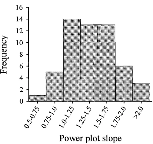
(24) Chapter Two -9reclassification error rates for each habitat class (i.e. the frequency at which transects would be assigned to other habitat classes). In order to identify the independent contributions of continuous vs categorical habitat variables in explaining patterns in the fish assemblage, Partial Canonical Correspondence Analysis (Ter Braak 1988) was used to partition the assemblage variation among habitat class (coded as dummy binary variables), benthic cover (square-root-transformed continuous variables), and their interaction (see Borcard et al. 1992, Syms in press, for a full description). The structure coefficients from the ordination were then plotted to depict relationships between the three sets of variables Fish, habitat class, and benthic cover.. 2.4 Results A total of 701 transects were sampled, and 42560 damselfish from 65 species were recorded. Only species which occurred in more than 10 sites were subsequently analysed, so 10 species were dropped from analysis and 55 species included in the ANCOVA. Twelve classes of physiographic habitat were identified a priori and could be broadly grouped into exposed vs sheltered, and reef top versus reef slope classes (Table 2.1). Sample effort was uneven across habitat classes and generally reflected the availability of that habitat around the island (Table 2.1). The distribution of individuals among species indicated that the pomacentrid assemblage on Lizard Island was diverse and relatively even (Fig. 2.1a) (Frontier 1985). The species-frequency distribution approximated the log-normal (Fig. 2.1b). Scale-dependence of damselfish populations The relationship between log(variance) and log(mean) did not differ between combinations of species and habitat (f-ratio derived from Type I sums of squares, 3-way interaction p=0.5901). However a significant interaction between species and habitat class (f ratio derived from Type I sums of squares, 2-way interaction p<0.0063), the presence of non-zero slopes and significant (covariate-adjusted) effects of habitat class and species (f ratios derived from Type III sums of squares, all p<0.0001) indicated species should be analysed separately. Separate ANCOVA' s conducted on each species indicated variance-mean relationships were generally not different between habitat classes. Only 2 of the 55.
(25) Chapter Two -10species analysed had statistically different slopes in different habitat classes -. Hemiglyphidodon plagiometapon (p=0.0014), and Premnas biaculeatus (p=0.0006). Subsequent examination of the data indicated this heterogeneity was due to habitats in which these species were present but rare (<4 occurrences). Dropping these sites from the analysis removed the difference in slopes. All but 7 species had significant log(variance)-log(mean) relationships. (Amblyglyphidon leucogaster, Chrysiptera. biocellata, Chrysiptera talboti, Chrysiptera taupou, Dischistodus melannotus, Pomacentrus pavo, Pomacentrus tripunctatus).. Examination of the Taylor plots. indicated that all these species had positive variance-mean relationships, but the strength of association was reduced by a combination of low numbers and outlier points. Because slopes for each species were not generally different in different habitats, I combined different habitat classes and calculated the combined slope for each species. Slopes were approximately normally distributed across an ecologically important range (0.51 to 2.09) (Fig 2.2). This indicated that different taxa ranged from highly overdispersed (small slope) to moderately aggregated (large slope) at the 30x10m scale.. Habitat classification In order to identify the relative roles of habitat classification versus benthic cover as descriptors of habitat, I measured the ability of benthic cover to predict which transect belonged to which class using Discriminant Function Analysis. With the exception of 3 pairs of habitats classes, the a priori classification scheme was adequately predicted by DFA of the benthic cover variables. Of the exceptions, Reef Top (Exposed) habitats were misclassed as Reef Slopes (Exposed) 12.7% of the time; and Reef Top (Sheltered) habitats were misclassed as Reef Slope (Sheltered) 21.8% of the time (conversely, Reef Slope (Sheltered) habitats were misclassed as Reef Top (Sheltered) 16.9% of the time). These pairs of habitats were separable by the physical criterion of depth, and so I retained the distinction between them. Reef Slope (Lagoonal windward) habitats were misclassed as Reef Slope (Lagoonal leeward) habitats 36.7% of the time (the converse misclassification occurred 6.7% of the time). The assymetry of the misclassification indicated that the benthic cover parameters were not completely overlapping, and consequently I retained the distinction between these classes also..
(26) Chapter Two -11Assemblage association with habitat Species richness varied with site and habitat class (Table 2.2). Site variability subsumed most of the variation (48.7%). There was no clear association between species richness and habitat class. The lagoon slope supported the greatest diversity of damselfishes (11.7%), and lagoonal back-reef habitat the least (2.7%) (Table 2.2). Most habitats were similar in their species richness with the exceptions of rubble, cliff-edge, and lagoonal back-reefs which were considerably depauperate in the average number of species per transect. At the family level, pomacentrid abundances were generally variable, with slightly less than a third of that variation explainable by habitat variables (habitat class and benthic cover in combination) (Fig 2.3). Benthic cover and habitat class were neither mutually exclusive nor completely overlapping in their explanatory ability. Benthic cover independently explained 8.7% variation, while habitat class independently explained 6.8%. Their interaction, however explained 12.8% of the variation. This interaction implied that habitat class and benthic cover should be used in combination, and do not provide independent measures of habitat. In other words, the relationship between fish and benthic cover data collected from samples allocated to zones cannot be unbiasedly estimated. Two main patterns in pomacentrid assemblage structure were apparent. The contrast between cliff-edge assemblages and all other habitat types accounted for the first portion of total variation. This pattern was driven by the dominance of Abudefduf species, Chrysiptera unimaculatus, and Pomacentrus tripunctatus in cliff-edge habitats (Fig 2.4a). The cliff-edge habitat class was found adjacent to the granite bluffs of Lizard Island, in shallow water and was exposed to various degrees of wave action. Benthic cover was generally bare rock (Fig 2.4c). The second portion of variation was driven by depth differences. Reef tops were characterised by a suite of species (Fig 2.4a), the degree of which was more extreme in the exposed reef top habitats (Fig 2.4b). Benthic cover on the reef tops generally consisted of large hard coral forms (plating, digitate, corymbose and encrusting corals) (Fig 2.4c). In contrast, reef slopes were not characterised by many species (except for Chrysiptera rollandi and Pomacentrus amboinensis), but were characterised by the absence of both the reef-top benthic cover types (i.e. hard corals), and pomacentrids..
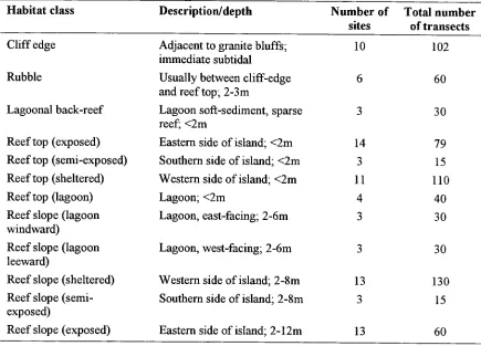
(27) Chapter Two -12-. Table 2.1. Habitat classes and sample allocation. Habitat class. Description/depth. Cliff edge Rubble Lagoonal back-reef Reef top (exposed) Reef top (semi-exposed) Reef top (sheltered) Reef top (lagoon) Reef slope (lagoon windward) Reef slope (lagoon leeward) Reef slope (sheltered) Reef slope (semiexposed) Reef slope (exposed). Number of sites. Total number of transects. Adjacent to granite bluffs; inunediate subtidal Usually between cliff-edge and reef top; 2-3m Lagoon soft-sediment, sparse reef; <2m Eastern side of island; <2m Southern side of island; <2m Western side of island; <2m Lagoon; <2m Lagoon, east-facing; 2-6m. 10. 102. 6. 60. 3. 30. 14 3 11 4 3. 79 15 110 40 30. Lagoon, west-facing; 2-6m. 3. 30. Western side of island; 2-8m Southern side of island; 2-8m. 13 3. 130 15. Eastern side of island; 2-12m. 13. 60.
(28) Chapter Two -13-. Table 2.2. Analysis of variance of species richness per transect. Source. DF. Type 111 SS. Mean Square. F Value. Pr > F. Habitat Class. 11. 3803.116705. 345.737882. 8.1683. 0.0001. Site (Habitat Class). 74. 3077.789619. 41.591752. 8.7968. 0.0001. 615. 2907.758333. 4.728062. Error. Tukey's HSD test: Variance component estimate of sites within habitat class (95% confidence interval): 48.655% (47.721 - 49.143%) reef slope (lagoon windward) reef top (lagoon) reef slope (semi-exposed) reef top (sheltered) reef slope (sheltered) reef top (exposed) reef slope (exposed) reef top (semi-exposed) reef slope (lagoon windward) rubble cliff-edge lagoonal back-reef. 11.67 10.93 10.60 9.85 9.61 9.27 9.12 8.20 8.03 5.88 4.82 2.73.
(29) Chapter Two -14-. 10. 100. Species rank. b) 16 14 12 c.)1. cucu. cr V t,. 10 8 6 4 2 0. moo%}'s?. .;" r,. '''. a. .:S' " & " 0 o'`7) ,.S'' c''''' ^.., 0 ° O. › Q'. '. o. ^) 0 0 •,,. Abundance class Figure 2.1. Species abundance distributions of pomacentrids. a) Rank-abundance plot, b) Frequency distribution.
(30) Chapter Two -15-. 420 I\4-) 0' 0. O 4-) N. rN? I\4') 0. 0'. N'. 4") rN,. 0 ey. 4-) >.. ti. <\. Power plot slope Figure 2.2. Distribution of slope parameters from power-plots of 55 pomacentrid species..
(31) Chapter Two -16-. 50. Percentage of variat ion. 40. Unexplained variation. 30 Habitat class 20 Benthic cover*habitat class 10 Benthic cover 0. Figure 2.3. Percent variance of the pomacentrid assemblage explained by benthic cover, habitat class and their interaction. Variance components obtained from partial Canonical Correspondence Analysis..
(32) Chapter Two -17-. 1.0 0.8. a) Fish species. 0.6. P.bankanensis P. d ckii C.rex S.agice/ fiactymatus .attipectoralis Piwaral A polvacanthus Polpidogenys. 0.4 0.2. Canon icalAxis 2 (1 5.1% o f explainable variation). 0.0 -0.2 -0.4. • : • Z. % P.moluccensis •• • ' t • A.curacao A. 1raigienwd'o; P.adelus Asordidus • u.ummaculatus A.septemfasciatus • %P.amboinensis P.tripunctatus •. C.rollandi. A.bengalensis. 1.0 0.8. Habitat class. Reef top (exposed). 0.6 0.4 Reef top (sheltered) Reef top (lagoon). 0.2. to. 0.0 -0.2 -0.4. Cliff edge. Reef slppe (lagoon leeward) .Reef ubb slope (exposed) Back reef Rubble Rplp..f since (sheltpred). 1.0 0.8 0.6 0.4 0.2. 0.0 -0.2 -0.4. Benthic cover Plating Digitate Corymbose Encrusting Staghom. Dead sghorn Bare rock ck Cobbles. massive. 0• I. • Branching 'foliose Oacroalgae. Sand. Rubble. -1.0 -0.8 -0.6 -0.4 -0.2 0.0 0.2 0.4 0.6 0.8. 1.0. Canonical Axis 1 (28.9% of explainable variation). Figure 2.4. Canonical Correspondence Analysis of pomacentrids with habitat class and benthic cover. Co-ordinates are structure coefficients. Filled symbols are points with axis correlations of <0.2..
(33) Chapter Two -182.5 Discussion The relationship between variability and the mean provides an estimate of the scale dependence of a population. A power-plot slope of 2 is the null model in which changes in variance are decoupled from changes in the mean abundance of an organism. In other words, population dynamics in small sample units with few organisms provide an unbiased estimate of the equivalent dynamics in large units with more individuals. Two competing models, both derived from terrestrial organisms, have been put forward to explain deviations in natural populations from this null relationship. First is a behavioural model (Taylor 1984) in which migratory and congregatory behaviours result in aggregations of organisms; second is a demographic-environmental heterogeneity model in which spatial pattern is seen as a stochastic interplay between population dynamics and environmental heterogeneity (Downing 1986). In this study I measured the variance-mean relationship within a family of coral reef fishes to establish if these populations are scale dependent. Because the power relationship does not exclusively distinguish between the models (Perry 1988), I also measured the contribution of environmental heterogeneity to explaining the patterns. These measures, in combination, yield insight into the mechanisms that may mediate scaling relationships within pomacentrids. Power relationships within and between-species form an important way of distinguishing the behavioural from the demographic-environmental heterogeneity model (Downing 1986). In the behavioural model, spatial variance is intrinsically regulated by the species and consequently the power-relationship 03) should be constant within species regardless of habitat (Taylor et al. 1980), and 13 should differ between species (Taylor et al. 1980, Taylor 1984). In addition, 13 may assume values above 2 (e.g. 3.8 in aphids (Taylor and Woiwod 1982)). In contrast, the demographicenvironmental heterogeneity model predicts that 13 should be constrained to lie between 1-2, and should differ within the same species in different habitats i.e. populations are extrinsically organised (Anderson et al. 1982). In reality, various model parameters can be manipulated so that 13 may assume a range of values and is not necessarily constrained in any model (Perry 1988). Consequently, support for either model requires a sound knowledge of the biology of the organisms. In this study, 13 ranged from 0.51-2.09, but generally ranged from 1-2 for most species (Fig 2.2). Species differed in their values of R, and in general these values were.
(34) Chapter Two -19consistent across habitats. These results are consistent with a behavioural model of spatial variability. However, two ecological characteristics of reef fish would caution against this interpretation. First, coral-reef fish are not renowned for undertaking largescale (in the order of kilometres) movements (Jones 1991). Given that damselfish are very small and sedentary, movement is even more unlikely. Second, coral reef fish have been widely documented as associated to some degree with habitat variables (Jones and Syms 1998, Appendix III), and so habitat should play some role in their distribution. Habitat (measured as a classification variable and benthic cover) explained approximately 30% of variation in the data set, which indicated that the behavioural model at best is probably only a partial explanation of the spatial variability in damselfish. The two models are not constrained to be mutually exclusive. Species-specific behaviour may act to moderate environmental-demographic stochasticity. Assuming species-specific habitat association such as is evident in this study (Fig 2.4), and relatively fine grained (at the scale of 100's of metres) spatial heterogeneity of habitats, species-specific. p. would be expected to lie within the range of 1-2 (Anderson et al.. 1982, Perry 1988). These data support a model in which environmental heterogeneity contributes to the variance-mean relationship of pomacentrids, but species-specific idiosyncracies serve to moderate the stochasticity that might be expected from a conventional population model. This finding is important when considering the scale-dependence of reef fish. As the slopes were generally less than 2, variability was therefore negatively associated with population size. In other words, small samples would be proportionally more variable than large samples. Simple extrapolation or interpolation of scales would lead to biased perceptions of the population, and ultimately the assemblage dynamics. The grain of the habitat will be an important contributor to this pattern. A 13<2 implied that the highdensity sites were more homogenous than would be expected under the null model i.e. species abundance from transects within a 'preferred' zone would be less variable than expected (Soberon and Loevinsohn 1987). Scaling will be, at least in part, a function of both the distribution of habitat and the strength and scales of association of fishes with that habitat. An important barrier to developing a 'science of scale' (Meentemeyer and Box 1987) will be the measurement of habitat. Physiographic 'zones' or other classification criteria are convenient sample devices, and many studies have found that within-zone.
(35) Chapter Two -20variability is far less than between-zone variability (Williams 1982, Russ 1984 a, b, Green 1986). However, determining which component of the 'zone' fish are responding to will be difficult due to the inherent confounding of benthic cover and habitat class. This difficulty is not improved by the observation that zone and benthic cover are not simply related to each other - they describe overlapping but not completely coincident patterns in data. In order for the independent components of each type of habitat measure to be identified and measured, a wide a range of habitat conditions incorporating a wide range of variability will need to be sampled. In conclusion, this study has shown that damselfish are clearly scale dependent, and as a consequence, naive scaling by simply multiplying patterns by a scaling factor will not be productive. Scaling will require a rational, empirically and biologically relevant set of rules. Habitat structure appears to be an important covariate of scaling patterns, and may provide a means by which scaling rules can be generated. Far from scaling being an esoteric, catch-all term, the scale at which fish are associated with habitats may provide a tractable means of incorporating scale into ecological theory of coral reef fish communities..
(36) Chapter Three -21-. Chapter 3: At What Scales are Reef Fish Associated with their Habitat? An Empirical Study. 3.1 Abstract Scaling is central to establishing the context of ecological studies, and providing an estimate of the generality of studies carried out at single scales. Scales of pattern are indicated by variance increases at particular scales. It has been hypothesised that coincident scales of variance peaks may indicate the scale at which different organisms interact, however this assumption has not been critically examined. In this study I measured the association of coral reef fishes on contiguous reef with benthic cover, physical structure, and location, at nine scales ranging from 9-225m 2 . Fish and habitat variables were measured to a resolution of 3x3m in 24 30x30m quadrats placed around Lizard Island, northern Great Barrier Reef, Australia. The 9m 2 squares were then progressively aggregated and associations between fish and habitat variables calculated. All fish species and habitat variables (with the exception of depth) were most variable at the finest scale. However, contrary to expectation, correlations between fish and habitat variables were generally not apparent at scales of less than 54-144m 2 . The scale at which correlations became evident varied with the type of habitat variables. Benthic cover and location associations were most evident at scales greater than 144m2 . Physical variables were generally not important on their own. In contrast, associations between fishes and combinations of habitat variables were apparent at smaller scales (>54m2) and were generally of greater magnitude than independent effects. These results indicate that the scale at which correlations are strongest correspond to the scales at which the likelihood that both fish and habitat variables are present in the same quadrat is maximised; and not necessarily the scale at which fish are responding to their habitat. 3.2 Introduction The association between organisms and their habitat is a fundamental parameter for ascertaining how populations and communities are organised (Bell et al. 1991). However, determining the strength and form of these associations is not a simple matter. Habitats are patchy at a range of scales (O'Neill et al. 1986, Addicott et al. 1987, Wiens 1989, Kotliar and Wiens 1990), and consequently observations of communities will be.
(37) Chapter Three -22scale-dependent (Schneider 1992, 1994). In addition, habitat patchiness is the product of many covarying biotic and abiotic factors, and isolating exactly which features of the habitat an organism is associated with may prove difficult if not impossible to resolve. Habitat association is likely to be a complex product of the scales of pattern of the habitat and the scales at which organisms perceive and respond to habitat variables. Reconciling different scales of patterns, and the relationships between habitat and organism presents a challenge to ecologists (McArdle et al. 1997). A considerable number of studies, employing a wide range of methodologies, have attempted to resolve scale-dependent patterns in populations of a wide array of organisms (Schneider 1992, Legendre and Fortin 1989, Legendre 1993). Of equal, if not greater ecological importance is to establish scale linkages between different elements of the system in question (e.g. Blanchard 1990, Pinckney and Sandulli 1990). For example, organisms may be patterned at the scale of physical processes (Schneider and Duffy 1985), with prey species (Schneider and Piatt 1986), or many other critical factors. Reconciling the scales of potentially interacting sets of variables is intuitively quite simple. Coincident scales of pattern in two sets of variables may be interpreted as correlative evidence that the variables share some scaling characteristic (Greig-Smith 1952, Schneider and Piatt 1986). One method of describing spatial pattern relative to scale is to measure how variability changes with increases in spatial resolution (or grain). Although variability should decrease with scale (Home and Schneider 1995), the variance of spatially structured organisms should increase as the sampling scale approaches that of the 'patch size' or spatial domain (Wiens 1989) of the organism. This approach was formalised by Greig-Smith (1952), and has received wide application (e.g. Yoshioka and Yoshioka 1989, Underwood and Chapman 1996). Coincident peaks in variance, may indicate common scales of interaction for different organisms (Schneider and Piatt 1986). Environments are spatially heterogeneous (Addicott et al. 1987), and much attention has been paid to establishing the scales and dynamics of environmental patchiness in a wide array of systems (e.g. Duggins 1983, Dayton et al. 1984, Clark 1991, Hanski et al. 1995, Collins and Barrett 1997). The scale at which habitats are structured is of great importance to the ecology of organisms associated with those habitats (Addicott et al. 1987) and it may be predicted that strongly-associated organisms should be tightly linked to the scale of habitat structure. Consequently, we would expect maximal correlation between habitat and habitat-associates at that characteristic scale. This has.
(38) Chapter Three -23strong implications for correlative and experimental studies. If the abundance of a habitat-responding (sensu Jones and Andrews 1993) organism can be viewed as a linear function of its habitat (in the sense of a linear model such as regression or analysis of variance), then the maximal explanatory power of the model should occur at the characteristic scale of their coincident variability peaks. Coral reefs are spatially heterogeneous over a range of scales (Williams 1991). Within a reef, the primary structure is typically a physiographic zonation pattern (Done 1992) corresponding to a combination of depth and aspect. Within a zone, corals form mosaics of coral-rich patches, interspersed with rubble, bare rock and a variety of other benthic cover types (Aronson and Precht 1995). Coral reef fish are a faunal element that is intimately associated with coral reefs, although the strength and form of this association is variable. Generally, reef fish communities are distinguishable between locations of differing physical conditions (Anderson et al. 1981, Williams 1982, Russ 1984a), and across physiographic zones such as back-reefs, reef crests, and reef slopes (Bouchon-Navaro 1981, Russ 1984 a, b, Meekan et al. 1995, Green 1996). However the strength of association between coral reef fishes and finer-scale elements of the habitat (e.g. coral cover, topography) has been more widely debated. A range of correlation strengths have been recorded - ranging from very weak (Roberts and Ormond 1987, Roberts et al. 1988, Fowler 1990, Booth and Beretta 1994, Cox 1994, Green 1996); to very strong associations (e.g. Bell and Galzin 1984, Bell et al. 1985, Findley and Findley 1985, Bouchon-Navaro and Bouchon 1989, Hart et al. 1996, Jones and Kaly 1996) with fine scale habitat elements. Comparisons of these studies are difficult due to confounding effects of physiographic zone (Syms in press, Jones and Syms 1998, Appendix III, Chapter 2). The scale at which studies are conducted has been widely acknowledged as a potential source of discrepancies between reef fish studies (Ogden and Ebersole 1981, Sale 1988). Despite this recognition, little explicit attention has been paid to the empirical effects of scale differences in reef fish studies (but see Syms 1995, Syms and Jones in press). Scales at which fish-habitat associations have been measured vary widely from less than 1m 2 (e.g. Sano et al. 1984, Clarke 1989), to >1000m 2 (e.g. Alevizon et al. 1985, Bouchon-Navaro and Bouchon 1989). Further studies have even compared fish and habitat measures taken from different scales (e.g. Bouchon-Navaro and Bouchon 1989, Grigg 1994). There are two major deficiencies in single-scale approaches. First, if the scale at which the fish and the habitat variables are.
(39) Chapter Three -24incommensurate, then the study will be predisposed to find little fish-habitat association. Second, different types of habitat variables are likely to exert effects at different scales. It would be expected that fine-grained responses (e.g. association with coral heads) would assume more explanatory power at smaller scale than would coarsergrained responses such as zonal associations. In order to measure the scales at which fishes are associated with different types of habitat variables it is necessary to both alter the scale at which association is measured, and remove the potential confounding between habitat types (e.g. some corals may be found only at certain depths or locations). In this study, I alter the scale of resolution at which I measure habitat association of coral reef fishes. I consider 9 resolution scales ranging from 9m2 to 225m2. Associations between fish and three habitat types: benthic cover (e.g. hard coral growth forms, soft corals, rubble, bare rock etc.); physical structure (i.e. the depth and topography); and locality; were measured at each scale. To remove confounding of habitat types, I derived independent and interaction fractions for each combination of factors. In other words, I statistically derived the variation that could be attributed to benthic cover, physical structure, and locality - each operating in isolation, versus the variation that could be explained by one type of habitat measure conditional on another habitat type being present. Samples were taken from a wide range of localities to enable these independent and interactive effects to be isolated. The scales at which different types of habitat measures assume greater importance will suggest hypotheses about the scale at which these fish assemblages are structured. 3.3 Methods. This study was carried out at Lizard Island (14°40'S 175°27'E) on the northern Great Barrier Reef, Australia. Three 30x30m quadrats were placed on contiguous reef at each of 8 locations around the island resulting in 24 replicates (Fig. 3.1). Quadrats were established by placing a 30m baseline parallel to the shore, incorporating both reef slope and reef top habitats, to a maximum depth of 12 m, then triangulating the 30x30m quadrat from the baseline. Measuring tapes were then laid at 1.5m intervals parallel to the baseline to provide a reference for fish counts and physical measures. Fish, benthic cover, and depth variables were recorded from each 3x3m area within of the quadrat. Four fish families were counted: Damselfishes (Pomacentridae), Wrasses (Labridae), Butterflyfishes (Chaetodontidae), and Angelfishes.
(40) Chapter Three -25(Pomacanthidae). These groups include a wide array of fish sizes and trophic groups. Continuous lm wide video transects were recorded along each 1.5m lane and benthic cover subsequently measured from 20 random points per 3x3m square. Depth measurements were taken using a dive computer at 1.5m intervals along each transect tape. Adjacent 3x3m squares were progressively aggregated to give fish-habitat measurements at 9 different scales: 3x3m (9m 2); 3x6m (18m2), 6x6m (36m2); 6x9m (54m2); 9x9m (81m2); 9x12m (108m2); 12x12m2 (144m2); 12x15m (180m2); and 15x15m (225m2). Fish data were square-root transformed to reduce the influence of absolute abundance. The benthic cover data were converted to proportions, and the most abundant cover categories retained for further analysis. In order to separate depth per se from topography, a quadratic response-surface analysis was applied to the raw depth data. The predicted values from the response-surface regression corresponded to the `typical' depth of a point. The deviation of the observed depth from the predicted depth gave a measure of topography. This gave the ability to distinguish between depressions or high features at any given depth (e.g. a high feature in deep water was distinguishable from a depression in shallow water). In order to accomodate non-linear patterns (e.g. association with intermediate depths or topography) a set of polynomial variables was derived from both predicted depth and topography by first standardising and then calculating: depth2, topography2, depth*topography, depth2*topography, depth*topography2, and depth2*topography2. These parameters were standardised to zero mean and unit variance and included in the analysis resulting in 8 physical variables. Location around Lizard Island was coded as 7 dummy binary variables. Analysis The primary aim of the analysis was to ascertain how much of the variation in distributional patterns of fishes in the environment can be attributed to 3 sets of variables: benthic cover, location, and physical structure; and to determine at which scales these parameters are important. Multiple regression was used to directly evaluate the association between fish and these habitat variables. The approach of Whittaker (1984) was used and entails running a series of regressions to partition the residual sums of squares among interaction and simple effects, expressing these fractions as proportions of the total variation in the data set. This method is discussed by Whittaker (1984) for univariate regressions, and Borcard et al. (1992) for multivariate applications..
(41) Chapter Three -26All species were analysed separately, rather than using a multivariate approach. There were two reasons for this. First, an important assumption of the multivariate approach (e.g. Borcard et al. 1992, Belgrano et al. 1995 a b, Syms in press) is that all species have a similar form of response to the independent variables (Ter Braak 1995). Second, the multivariate approach requires extensive quantities of data and would restrict the number of scales that could be considered due to the decrease in replication as squares were aggregated with each increase in scale. The percentage of variation explained by the regressions was calculated for each species and each scale. To further summarise the data, I carried out a divisive clustering process based on similarity of the two largest variance portions at each split. Mean values and standard errors of the variance fractions of each cluster were then calculated and presented. Ascertaining the significance of the fractions was problematical. The large numbers of regressions calculated makes interpretation of individual statistical tests prone to Type I error, in addition the estimates derived were not independent of those from other scales. More importantly, the biological importance of a given fraction is unclear. Preliminary tests sets indicated approximately 10% of variation could be accounted for by random variables alone, consequently I treated 10% as an approximate significance level.. 304 Results Habitat and fish abundance variability Although sample grids were placed so as to contain both reef slope and reef top habitats, the 'typical' zonation pattern was not a general profile (Fig. 3.1). The transition from reef top to reef slope was sharper at sites on the eastern side of the island, in contrast with the western sites in which the transition was gentler. The response-surface regressions modelled the depth profiles well (mean r-square = 0.823 ± 0.026), indicating that both long-range (depth) and short-range (topography) components could be reliably extracted from the depth data. Although the depth range was greater on eastern sites, average depths were similar regardless of the side of the island, indicating that no systematic depth bias was present (Fig. 3.2). Average topography was also consistent among sides of the island, with the exception of northeastern sites which had a greater topographic complexity (Fig. 3.2). The variance of the physical reef structure decreased with increases in scale. Depth variability was.
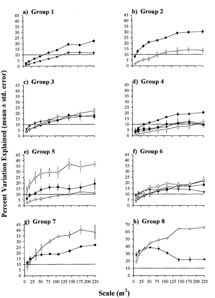
(42) Chapter Three -27consistently high at smaller scales but decreased sharply between 54-81m2 (Fig. 3.3) to assume a new, relatively constant level. In contrast, topographic variability underwent a monotonic decrease, with the greatest changes occurring at the smallest scales (Fig. 3.3). Benthic cover differed between sides of the island. Eastern sites were characterised by encrusting, branching, corymbose, and plating hard corals (Fig. 3.4). In contrast, western and lagoonal sites were typified by more gravel and sand, staghorn corals, branching soft corals, and macroalgae (Fig. 3.4). However, site clusters overlapped considerably so that cluster membership was not exclusively represented by a typical benthos. Two characteristic variability profiles were apparent among the benthic categories (Fig. 3.5) and reflected the grain of the benthic type. The gently decreasing profile was typical of evenly distributed and large patch forming categories (bare rock, sand, rubble, macroalgae, massive soft coral, plating, digitate, staghorn hard coral). In contrast, the sharper decrease of the second profile was characteristic of sparsely distributed and patchy categories (turf algae, dead corals, massive, encrusting, caespitose, corymbose, branching hard corals). As with the habitat parameters, the proportional variance of all fish species in each family decreased sharply with increasing scale (Fig. 3.6). This pattern may represent one of two things. Either patchiness was present outside the bounds of the sampling grain (ie less than 9m2 or greater than 225m2) or the fishes were simply sparsely distributed.. Fish-habitat association. Pomacentrids Within pomacentrids, eight types of habitat association were identified. Group 1 contained 18 species from 11 genera (Table 3.1) which were correlated with primarily with benthic cover variables (maximum 22% variation explained), and to a lesser extent, location around the island (maximum 12% variation explained) (Fig. 3.7a). The strength of association with each factor increased monotonically with scale and levelled at >144m2 . The species making up this group were not necessarily ecologically similar, and included shoaling planktivorous species, live-coral associated species, and sand/rock associated species (Table 3.1)..
(43) Chapter Three -28Group 2 consisted of six species from five genera, which were strongly associated with benthic cover, to some extent conditional on locality (Fig. 3.7b). As with the previous group, the strength of association with both factors increased monotonically with scale. The explanatory power of benthic cover increased rapidly to reach 21% at 54m2, then gently increased to plateau at 144m 2 (30% variation explained). The benthic cover*locality interaction was far smaller (to 14%) and only became significant at larger scales. The species forming this group were not strongly ecologically similar - some were associated with sand, others with branching and staghorn corals (Table 3.1). However, all species were associated with either back-reef or lagoonal locations. Group 3 consisted of six species in five genera which were associated with benthic cover and locality - both as independent fractions, and as interactions (Fig. 3.7c). Each portion of variation increased gradually with scale and approached approximately equal maxima (18-20% variation explained). There was no ecological similarity in the component species which included lagoonal, back-reef and exposed localities and a range of benthic cover associations (Table 3.1). Group 4 consisted of four species in three genera which were weakly associated with benthic cover (maximum 20% variation explained), an association that increased gradually with scale (Fig. 3.7d). In addition, location, physical variables, and their interactions accounted for smaller portions of variation (maximum 12%). In isolation, these portions were barely significant but when viewed as a suite of related factors explain up to 36% of the variation. In contrast with the previous groups, the species in group 4 were ecologically similar and were found on shallow reefs in association with hard corals (Table 3.1). However at a finer level of benthic association, the species were ecologically different.. Pomacentrus chrysurus, Pomacentrus coelestis and. Stegastes nigricans were weakly associated with digitate, corymbose and massive corals respectively, while Plectroglyphidodon dicki was associated with a suite of plating and branching coral types. Group 5 was composed of three species from two genera which were characterised by a strong association with benthic cover conditional on the physical structure of the reef (Fig. 3.7e). The variance portion accounted for by the interaction was evident even at the smallest scale, and increased rapidly to an initial plateau of 29% at between 54108m2, and increased again to the final plateau (37% explained) at the 144m2 scale. Variation attributable to benthic cover alone was lower than the interaction (19% explained), but reasonably constant above 81m 2. A small (12%) location effect,.
(44) Chapter Three -29contingent on habitat, was also evident at the largest scales. Two of the species that made up the group, Pomacentrus bankanensis and Stegastes fasciolatus, were associated with depressions in shallow reefs, and digitate corals (Table 3.1); while the other species (Pomacentrus amboinensis) was associated with high features in deeper, macroalgal and rubble dominated areas. Group 6, consisting of 3 species in 2 genera, was characterised by a complex suite of associations with benthic cover, location, their interaction, and a benthic cover*physical variable interaction (Fig. 3.7f). All factors were of a similar magnitude (15-22% variation explained) and reasonably constant at scales above 81m2. Three species that formed this group were ecologically complementary. Chrysiptera rex and Pomacentrus wardi were both shallow water dwellers, associated with hard branching and plating coral forms (Table 3.1). However, C. rex was generally found at more exposed localities (Washing Machine) than P. wardi, which was found more in back-reef and semi-exposed localities (Osprey and Palfrey). In contrast, Chrysiptera rollandi was generally found in deep-water at back reef and lagoonal localities and was associated with staghorn corals, macroalgae, sand, and soft corals (Table 3.1). Group 7 contained two species which were strongly associated with benthic cover, contingent on locality (Fig. 3.7g). The benthic cover*locality interaction rose sharply to plateau above 108m 2, to maximum value of 40% variation explained. Benthic cover association alone was evident from a small scale (18% at 36m 2) and reached 27% at the largest scale. Both species in the group were found in back-reef and lagoonal habitats. Amblyglyphidodon curacao was associated primarily with staghorn corals, Pomacentrus adelus with soft and dead hard corals (Table 3.1). Group 8 consisted of two species,. Hemiglyphidodon plagiometapon. and. Pomacentrus grammorhynchus. At smaller scales (9-54m2) location explained most of the variation (maximum 38% variation explained) but then dropped to 20% at the 144m 2 scale (Fig. 3.7h). At larger scales, the explainable portion of the variability was subsumed by the benthic cover*location effect which plateaued at 144m2 to explain a maximum of 66% variation. Both species were ecologically similar; being strongly associated with staghorn corals, contingent on that habitat being in the lagoon (Table 3.1)..
Figure

+7
Related documents