Theses Thesis/Dissertation Collections
6-2017
Deep Liquid State Machines with Neural Plasticity
and On-Device Learning
Nicholas M. Soures
Follow this and additional works at:https://scholarworks.rit.edu/theses
This Thesis is brought to you for free and open access by the Thesis/Dissertation Collections at RIT Scholar Works. It has been accepted for inclusion in Theses by an authorized administrator of RIT Scholar Works. For more information, please [email protected].
Recommended Citation
Nicholas M. Soures June 2017
A Thesis Submitted in Partial Fulfillment
of the Requirements for the Degree of Master of Science
in
Computer Engineering
Nicholas M. Soures
Committee Approval:
Dr. Dhireesha Kudithipudi Advisor Date Professor, Computer Engineering
Dr. Andreas Savakis Date
Professor, Computer Engineering
Dr. Brad Aimone Date
I would like to take this opportunity to thank my advisor, Dr. Dhireesha
Ku-dithipudi, who has provided valuable support and has been an amazing mentor
throughout this work. I would also like to thank my committee members Dr. Andreas
Savakis and Dr. Brad Aimone for their time and support and am very appreciative
for their insightful comments.
I’d like to thank Dr. Ernest Fokou´e for his helpful discussions. I also wish to
extend my thanks to Dr. Cory Merkel for his expert advice.
The RIT Computer Engineering Department's faculty and staff, namely, Richard
Tolleson, Emilio Del Plato, Richard Flegal, and Lourdes Marquez-Douglas for their
help computing resources and logistics.
Also, I would like to thank all my lab members, especially Abdullah M. Zyarah
and Luke Boudreau who have provided valuable feedback and help in this work.
Finally, I would like to take this opportunity to thank my loving parents, brother,
sisters, and other family members who have supported and provided so much for me.
Without them this would not have been possible. Also, I would like to thank my fianc´e
The Liquid State Machine (LSM) is a recurrent spiking neural network designed for
efficient processing of spatio-temporal streams of information. LSMs have several
inbuilt features such as robustness, fast training and inference speed, generalizability,
continual learning (no catastrophic forgetting), and energy efficiency. These features
make LSMs an ideal network for deploying intelligence on-device.
In general, single LSMs are unable to solve complex real-world tasks. Recent
literature has shown emergence of hierarchical architectures to support temporal
in-formation processing over different time scales. However, these approaches do not
typically investigate the optimum topology for communication between layers in the
hierarchical network, or assume prior knowledge about the target problem and are
not generalizable.
In this thesis, a deep Liquid State Machine (deep-LSM) network architecture is
proposed. The deep-LSM uses staggered reservoirs to process temporal
informa-tion on multiple timescales. A key feature of this network is that neural plasticity
and attention are embedded in the topology to bolster its performance for complex
spatio-temporal tasks. An advantage of the deep-LSM is that it exploits the random
projection native to the LSM as well as local plasticity mechanisms to optimize the
data transfer between sequential layers. Both random projections and local plasticity
mechanisms are ideal for on-device learning due to their low computational
complex-ity and the absence of backpropagating error. The deep-LSM is deployed on a custom
learning architecture with memristors to study the feasibility of on-device learning.
The performance of the deep-LSM is demonstrated on speech recognition and seizure
Signature Sheet i
Acknowledgments ii
Dedication iii
Abstract iv
Table of Contents v
List of Figures viii
List of Tables 1
1 Introduction 2
1.1 Motivation . . . 2
1.2 Objectives . . . 5
1.3 Outline . . . 6
2 Background and Relevant Work 7 2.1 Liquid State Machine . . . 7
2.1.1 LSM Algorithm . . . 8
2.1.2 Example of LSM Dynamics . . . 13
2.2 Relevant Literature . . . 16
2.2.1 Processing multiple time-scales of information . . . 16
2.2.2 Attention . . . 20
2.3 Neuromemristive Computing . . . 20
2.3.1 Memristor Device . . . 21
2.3.2 Crossbar Architectures . . . 22
2.3.3 Noise . . . 25
2.4 Summary . . . 26
3 Proposed deep-LSM Architecture 27 3.1 Liquid Layer Optimization . . . 28
3.2 Clockwork-LSM . . . 31
3.3.1 Feedforward deep-LSM . . . 34
3.3.2 Unsupervised deep-LSM . . . 36
3.4 Attention Mechanism . . . 41
3.5 Summary . . . 43
4 Neuromemristive LSM Design 45 4.1 Input Layer . . . 46
4.2 Random Spiking Layer . . . 46
4.2.1 Memristor Crossbar Core . . . 47
4.2.2 Leaky Integrate-and-Fire Neurons . . . 49
4.2.3 Ziksa for Initialization and STP . . . 49
4.3 Unsupervised Spiking Layer . . . 51
4.3.1 STDP with Ziksa . . . 51
4.3.2 Intrinsic Plasticity Block . . . 52
4.4 Readout Layer . . . 53
4.5 Summary . . . 56
5 Simulation Methodology 57 5.1 Simulation Methodology . . . 57
5.2 Optimal LSM Architecture . . . 58
5.3 Seizure Detection Dataset . . . 59
5.4 Speech Recognition Dataset . . . 59
5.5 Neuromorphic Noise Analysis . . . 60
5.5.1 Memristor Noise Models . . . 60
5.5.2 High-level Noise Analysis . . . 61
5.6 Summary . . . 62
6 Results and Discussion 63 6.1 Analysis of Optimal Liquid Layer . . . 63
6.2 Analysis of Optimal deep-LSM Model . . . 65
6.2.1 Performance on Speech Classification . . . 65
6.2.2 Robustness of deep-LSM Models . . . 68
6.2.3 Performance of Top Models on Larger Speech Classification . . 73
6.2.4 Analysis of Unsupervised deep-LSM . . . 75
6.2.5 Comparison to State-of-the-Art . . . 77
7 Conclusions and Future Work 79
7.1 Conclusion . . . 79
7.2 Future Work . . . 80
2.1 High-level architecture of LSM network. . . 8
2.2 Behavior of Leaky Integrate-and-Fire neuron with random input. . . . 9
2.3 Projection of low-dimensional input into high-dimensional liquid layer. 10 2.4 Using a classifier to classify based on the state of the LSM. . . 13
2.5 Synthetic temporal detection task of five different input patterns ran-domly generated with a Poisson process. . . 14
2.6 Accuracy of LSM on synthetic dataset for different degrees of connec-tivity between the input layer and the liquid layer. . . 14
2.7 Accuracy of LSM on a synthetic dataset with an increasing number of failing neurons in the liquid layer. . . 16
2.8 Hysteresis curve of a ReRAM device switching between an On and Off resistance state (Device figure from [1]). . . 21
2.9 Generic crossbar architecture of memristive devices capable of perform-ing vector-matrix operations. . . 23
2.10 Ziksa being used to set/reset a memristor in a crossbar setting. . . 25
3.1 Architecture of proposed deep-LSM. . . 27
3.2 Sparse projection from the input layer to the liquid layer. . . 29
3.3 Sparse connectivity of a 10x10 liquid layer using (2.3) withλ= 4. . . 29
3.4 Comparison of STP model in [2] to the proposed STP model. . . 30
3.5 STP model according to (3.1) as a function of the pre-synaptic action potentials with α= 0.01 and β = 0.3. . . 31
3.6 A liquid layer in the Clockwork-LSM consists of neurons with differ-ent time constants and thresholds which causes neurons to integrate information on different time-scales. . . 32
3.7 A percentage of neurons in the liquid layer are randomly selected as backbone neurons. In the proposed deep-LSM models, the sequential liquid layers are all the same size and the backbone neurons are the same in each liquid. . . 34
3.8 Architecture for a deep-LSM consisting of a chain of liquid layers. . . 35
3.10 Architecture for a deep-LSM consisting of an intermediary feedforward
network randomly connected to the next liquid layer. . . 36
3.11 Architecture for a deep-LSM consisting of an intermediary feedforward
pooling layer randomly connected to the next liquid layer. . . 37
3.12 Architecture for a deep-LSM consisting of an intermediary
feedfor-ward unsupervised layer randomly connected to the next liquid layer
(Dashed lines represent trained synapses). . . 37
3.13 Architecture for a deep-LSM consisting of an intermediary feedforward
unsupervised pooling layer randomly connected to the next liquid layer
(Dashed lines represent trained synapses). . . 38 3.14 A subsection of synaptic strengths after training for unsupervised
clus-tering on MNIST. (a) A few neurons inhibit all others from learning.
(b) Every neuron shows that it is learning, however learning is
dom-inated by neurons which fire to every class. (C) Only a few neurons
learn to respond to every input class. (d) Each neuron learns a specific
number. (Figure based on results in [3, 4]). . . 40
3.15 Attention can be applied to the whole deep-LSM network which is the
deep attention mechanism (left) and spatially to a single liquid layer
which is the spatial attention mechanism (right). . . 41 3.16 Application of both attention networks to the deep-LSM architecture. 44
4.1 High-level architecture of blocks in the neuromemristive design of
deep-LSM with random encoding layers. . . 45
4.2 High-level architecture of blocks in the neuromemristive design of
deep-LSM with unsupervised encoding layers. . . 46
4.3 Block diagram of the spiking layer neuromemristive architecture where
the memristor crossbar core performs the synaptic multiplications, a
row of analog leaky integrate-and-fire neurons accumulate and process the inputs, and an analog write scheme known as Ziksa is used to set
the synaptic strengths and regulate STP. . . 47
4.4 Demonstration of how a crossbar can be used to perform the multiply
and accumulate operation in a neural network. . . 48
4.5 Mapping a single liquid layers synapses (with N inputs and M outputs)
to a M x N memristor crossbar core. . . 48
4.7 Logic flow for digital controller to perform synaptic normalization with
Ziksa. . . 50
4.8 Block diagram of the feedforward unsupervised spiking layer architecture. 51
4.9 Intinsic plasticity block which integrates with analog LIF neurons. . . 52
4.10 Block diagram of the readout layer architecture. . . 53
4.11 The first step of the attention mechanism is to set the memristors along
the diagonal of the N x N meristor crossbar cores to the corresponding
coefficients inASpatialfrom (3.13) such that Rn,n
Mn,n =An. This will result
in a group of identical crossbars for each liquid layer in the deep-LSM. 54
4.12 The second step of the attention mechanism is to scale each crossbar according to the corresponding coefficient ADeep from (3.11). This
results in the diagonal elements of each memristor crossbar core being
equivalent to the attention coefficient for the N neurons in the liquid
layer. By multiplying the outputs of the neuron in the liquid layer
with their respective memristor crossbar core we can obtain the final
representationX−F to be sent to the output layer. . . 55 4.13 The last step of the attention mechanism is to compute the final
repre-sentation of the deep-LSMXF to be used as input to the output layer.
The encoded deep-LSM state X−F is multiplied with the memristor crossbar core in the output layer which represents Wout to determine
y(n). . . 55
5.1 Datflow in MATLAB used for verification of the software deep-LSM
(left) and hardware emulation of the deep-LSM (right). . . 57
5.2 Measured resistance over 1000 different read pulses for aT iN−T aOx− T aT iN device. The data and figure were provided by Dr. Marinella’s
group at Sandia National Laboratories. . . 61
5.3 Average change in resistance ofT iN−T aOx−T aT iN memristor when
applying 60ns pulses of different magnitudes from a starting resistance
of 5kΩ. . . 61
6.1 Distribution of liquid layer size for top performing LSMs in both
ac-curacy and separation. . . 64
6.2 Distribution of degree of connectivity between input layer and liquid
layer for top performing LSMs in both accuracy and separation. . . . 64
6.3 Distribution of β in (3.1) for top performing LSMs in both accuracy
2.1 Comparison of scalability between Ziksa and other NMS write schemes. 25
6.1 Hyper-parameters analyzed for impact on performance and separation
of the LSM on a synthetic application. . . 63
6.2 Performance of deep-LSM models on 4-phoneme classification task. . 66
6.3 Performance of single LSM models for the 4-phoneme classification task. 67
6.4 Comparison of mean accuracy and standard deviation for deep-LSM
models and a large LSM with 2% input connectivity on the isolated
4-phoneme recognition task. The Unsupervised deep-LSM had the best
performance with the lowest standard deviation. . . 68
6.5 P-values from ANOVA for comparing themeans of the deep-LSM
mod-els and the large LSM on the 4-phoneme recognition task. . . 69 6.6 Noise analysis of deep-LSM models on the 4-phoneme classification task. 71
6.7 Scalability comparison of Unsupervised deep-LSM vs. a large LSM for
different memristor crossbar implementations. . . 72
6.8 Performance of top three deep-LSM networks on the 39-phoneme
clas-sification task compared to a large LSM and their standard deviation. 74
6.9 P-values from ANOVA for comparing the mean between the top
deep-LSM models and a large deep-LSM on the 39-phoneme recognition task. . 74
6.10 Noise analysis for the Unsupervised deep-LSM model compared to a
large LSM. . . 74 6.11 Analysis of a five layer Unsupervised LSM and Dual-Path
deep-LSM compared to the three layer deep-deep-LSM network. . . 76
6.12 Analysis of simplified attention model for different applications. . . . 77
6.13 Comparison of the Unsupervised deep-LSM to SOTA in RC and in
Introduction
1.1
Motivation
Artificial neural networks (ANNs) are parallel information processing systems that
can be optimized to approximate a function mapping a variable X to a new space
Y. The process of optimizing the ANN involves training the connections within the
network to achieve the best approximation as measured by a defined objective
func-tion. This principle can be applied to many real-world problems where ANNs can
learn mappings between audio signals and words [5, 6], visual information and
ob-jects [7, 8, 9], and bio-medical signals and health status of an individual [10]. As
ANNs progress, the range of real-world application spaces in which they can be
uti-lized is growing drastically. A majority of these emerging application domains are
spatio-temporal in nature and a class of neural networks known as recurrent
neu-ral networks (RNNs) are specifically designed to process the temponeu-ral information.
These networks need to process complex spatio-temporal signals where information
can exist on several time-scales.
The state-of-the-art in RNNs is Long Short-Term Memory (LSTM) [11], which has
achieved successful results in applications such as image captioning [12], text sequence
generation [13], and speech processing [14]. Though this network achieves
due to the large amount of memory and resources required to implement and train
LSTM networks. Training an LSTM is achieved with a learning rule known as
back-propagation-through-time. This learning rule requires a large amount of memory
to store the different states of the network over time, as well as a large number
of computations to update the network. The overall complexity and size of LSTM
networks limit the size of networks which can be implemented on embedded systems.
This in turn can limit the performance that can be achieved on a given application.
The long training time of LSTM networks can also be a limiting factor in systems
which need to constantly adapt to their environment or do not have sufficient amounts
of labeled data. A solution to avoid the large resource requirement for training is to
train a network offline. However, there are several applications that require training
and inference to be performed on the device or where a system cannot connect or
communicate to the cloud but needs to maintain full functionality. An example of
this is deploying unmanned vehicles to explore the ocean depths or foreign planets.
In general, systems with on-device learning have low latency in learning, low power
consumption, and are more secure. However, to deploy on-device the algorithm has
to be computationally light.
The need for light RNNs with reduced training complexity led to the development
of a class of networks known as reservoir computing (RC). RC was proposed in the
early 2000s by two research groups independently. The two networks are the Echo
State Network (ESN) proposed by Jager [15] and the Liquid State Machine (LSM)
proposed by Maass [16]. RC networks are three layer recurrent neural networks which
consist of an input layer, a reservoir, and a readout layer. The advantages of RC is
that only the weights from the reservoir to the readout layer need to be trained. This
avoids the long and costly computations required by gradient descent approaches such
as back-propagation-through-time and also avoids the vanishing gradient problem
LSTM requires four times as many weight parameters as reservoir computing networks
with much longer training times for networks of the same size. Due to their reduced
memory requirements and low cost training, RC is inherently suitable for embedded
platforms with on-device learning.
This work specifically focuses on the LSM for several reasons. The main difference
between the LSM and the ESN is that the LSM is a biologically inspired spiking
neu-ral network (SNN). Research in the dynamics and information-processing using the
LSM can accelerate simulations of neural systems for studying dynamics of neuron
interaction and modeling of advanced processes in the brain [17]. The process of
com-puting in spikes yields several advantages for neuromorphic comcom-puting with on-device
learning. Low-precision communication of spiking neural networks is advantageous
in hardware. We have shown that these networks are robust to internal noise [18],
making them a natural choice for neuromorphic systems. Lastly, literature shows that
communicating through spikes is energy efficient [19]. In [20] they proposed an analog
sigmoid neuron with a power consumption of 192.63µW in 180nm technology while
in [21] an analog spiking neuron was implemented which consumed 0.2-7nW at 90nm
technology. Arguably, another benefit of LSM is that individual spikes encode richer
information within the timing of spikes, which cannot be achieved in a rate-based
neural network [22]. In [23] the computational power of spiking neurons was shown
to be at least as powerful as sigmoid and threshold neurons if not greater.
The current LSM models are severely limited in performance and applicability to
real-world problems. One reason behind this is the limitation imposed by a single
dynamical layer driven by the input space [24, 25]. This limits the capabilities of the
LSM and results in needing very large reservoir systems to solve trivial tasks. This
work seeks to address how current limitations in performance can be overcome through
a deep and wide LSM (deep-LSM) inspired by the brain for hierarchical processing of
which has been linked to processing across scales and abstract concepts [26, 27] and
is needed to capture the information in real-world applications over multiple
time-scales [28]. Another feature seen in biological systems is attention. Attention allows
the brain to selectively process a multitude of visual stimuli and only focus on
selec-tive information to maximize its limited computational resources [29]. By applying
attention on the spatial representation of the reservoir, it is expected to improve the
performance of the readout layer by optimizing the networks ability to process all the
information in the deep-LSM.
This thesis will focus on improving the computational power of an LSM. Another
important goal is to study the efficiency of deploying on a neuromemristive system
(NMS). A NMS is a brain-inspired computer architecture which uses memristive
de-vices [1]. The contributions of this work are a new architecture called deep-LSM
which is a modification to the existing framework of the LSM, as well as an
explo-ration of plasticity mechanisms. Synaptic plasticity in the brain is important for the
development of memory and ability to process temporal information [30, 31]. The
proposed network is suitable for on-device learning in embedded platforms and
specif-ically tested on NMS. The algorithm is verified using speech and EEG benchmark
datasets. A high-level model of the proposed network is verified and tested for
de-vice variability and noise due to the characteristics of the memristive dede-vices. This
will show how the proposed network is more computationally efficient than using a
large reservoir and the robustness of the network which are two important criteria for
on-device intelligence. Over the course of this work there have been several relevant
publications in which I am the first author [4, 3, 18, 32] or have been a co-author
[33, 34, 35, 36].
1.2
Objectives
• Incorporate attention in the deep-LSM to enhance on-device learning.
• Study plasticity mechanisms to improve the performance of the deep-LSM in a
neuromemristive system
• Study the performance and robustness of the deep LSM with specific benchmark
datasets.
• Feasibility study for on-device intelligence in NMS.
1.3
Outline
The rest of this document is as follows: Chapter 2 presents background and relevant
research on the LSM, work on multi-time scale and hierarchical RNNs and RC,
mem-ristors, and neuromemristive architectures. Chapter 3 introduces the proposed
deep-LSM with the different architectures explored and several optimizations. Chapter 4
describes the building blocks of the neuromemristive system and how they would be
used to implement the full architecture. Chapter 5 discusses the benchmark datasets
and simulations used to verify the deep-LSM. Chapter 6 presents demonstrates the
robustness and performance of the deep-LSM. Chapter 7 concludes this thesis with
Background and Relevant Work
This chapter is broken into two main sections on the algorithm and hardware
respec-tively. The first section introduces the LSM in-depth along with relevant research that
has inspired the development of the deep-LSM. The second section introduces several
relevant architectures and a device known as a memristor which is fundamental to
the proposed architecture.
2.1
Liquid State Machine
The LSM is recurrent spiking neural network proposed by Maass in 2002 [16]. The
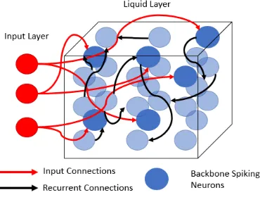
LSM consists of three layers: an input layer of neurons, a liquid layer of recurrently
connected spiking neurons, and a readout layer which is trained to decode the
infor-mation in the liquid layer. A high-level figure of the LSM is shown in Figure 2.1. The
theory behind the LSM, and RC in general, is that the input space can be transformed
by a random projection to a much higher dimensional space (the liquid). Projecting
the input into a higher dimension will facilitate learning by making the data more
lin-early separable. The recurrent connections in the liquid introduce feedback, making
the liquid layer a dynamic high-dimensional space which contains information of not
only its current inputs, but also the inputs within some past window of time. This
property is known as fading memory and the length of this memory is dependent on
Figure 2.1: High-level architecture of LSM network.
The LSM can be conceptually thought of as a bucket of water [37]. When an
input, say a pebble, is thrown into the surface of this water it will cause a disturbance
resulting in ripples across the surface. If another pebble is then thrown into the liquid,
the disturbance caused by the second pebble will interfere with the ripples caused by
the first pebble. This complex pattern that forms on the surface is encoding of all the
information about the timing between the two pebbles hitting the water, their size
and velocity, and the locations at which they disturbed the surface. By viewing this
encoded representation, we then need to train a decoder to extract the information
we want to recover.
2.1.1 LSM Algorithm
The LSM has three different layers of neurons and three weight matrices which
de-scribe the pre and post-synaptic connections of the neurons in each layer. The first two
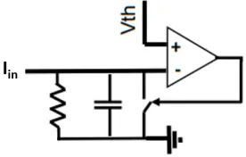
layers consist of spiking neurons. A common spiking neuron model used is the leaky
integrate-and-fire neuron model. The model simulates a neuron with a membrane
potential which integrates pre-synaptic action potentials. The membrane potential
The dynamics of the membrane potential can be described by (2.1).
τ∂V
∂t =−V +Iext∗R, (2.1)
where V is the membrane potential, τ is the membrane time constant, Iext is the
current induced by pre-synaptic action potentials and R is the membrane resistance.
Once the membrane potential V crosses a threshold the neuron emits an action
potential and the membrane potential resets to its resting state. After a neuron emits
an action potential it enters into a refractory period in which it cannot spike again
[image:23.612.248.399.300.412.2]for a short period of time as shown in Figure 2.2.
Figure 2.2: Behavior of Leaky Integrate-and-Fire neuron with random input.
The data flow through the LSM shown in Figure 2.3 starts with the input layer.
The input layer neurons are primarily used to convert external stimuli into the a
temporal spike train to be passed to the liquid layer (recent work has explored directly
injecting external signals as current into the network [35]). In order for the spike trains
to flow from the input layer to the liquid layer, it is necessary to define a weight matrix
describing the synaptic connections between the input layer (pre-synaptic) and the
liquid layer (post-synaptic). This connectivity weight matrix is generated randomly
from a uniform distribution with a constraint to enforce sparsity. In this approach,
if a connection is formed the weight is set to one. After this connectivity matrix is
the connectivity matrix can be computed by (2.2).
Iin(n) =Win∗u(n), (2.2)
where Win is the connectivity matrix from the input layer u(n) (the input signal
at time t=n) to the liquid layer and the product of the two is Iin(n) which is the
amount of current flowing into the neurons in the liquid layer at time t=n from the
[image:24.612.226.409.276.537.2]input layer.
Figure 2.3: Projection of low-dimensional input into high-dimensional liquid layer.
The second layer (the liquid layer) forms the high-dimensional transformation of
the input space. In the liquid there are two types of spiking neurons: excitatory and
inhibitory. Excitatory neurons promote activity within the network while inhibitory
neurons dampen the activity. The ratio between excitatory and inhibitory neurons
a mix of inhibitory and excitatory neurons equally spaced. In order to give the
liquid layer its inherent dynamic nature and memory, it is necessary to instantiate
a connectivity matrix describing the recurrent connections in the liquid layer. The
connections between neurons in the liquid are determined according to a probability
of a connection growing between two neurons based on the proximity of the neurons
given by (2.3).
Pr wresi,j 6= 0=Cexp (−D(i, j)/λ)2, (2.3)
where D represents the euclidean distance between the neurons i and j, λ is an
adjustable parameter that is used to control the degree of connectivity, and C is a
constant whose value is 0.3(EE), 0.2(EI), 0.4(IE), 0.1(II) as proposed in [16]. This
probabilistic method of connecting neurons results in small-world topology with dense
local connections and sparse global connections within the liquid which follow a
power-law distribution. The impact of the recurrent connections can be added withIinfrom
(2.2) to determine the total amount of current flowing into each neuron in the liquid
shown in (2.4).
Iext=Wrec∗x(n−1) +Iin(n), (2.4)
where Wrec represents the connectivity matrix for the recurrent connections and
x(n-1) represents the output of the reservoir neuron (1 if it fired, otherwise 0) from
the previous time step.
Though the connectivity matrix is never trained, the synaptic strengths of
connec-tions within the reservoir are modulated through short-term plasticity. Short-term
plasticity (STP) is a mechanism through which each neuron has limited synaptic
ef-ficacy. Therefore if a neuron recently emitted a spike, the synaptic efficacy of the
This can be modeled as a reduction in the synaptic strength (Wres). However, this
decrease is only temporary and decays back to full strength while the neuron is not
firing. This behavior can be captured by (2.5) and (2.6) proposed in [2].
Rn+1 =Rn(1−un+1)exp( −∆t
τrec
) + 1−exp(−∆t
τrec
) (2.5)
un+1 =unexp( −∆t τf acil
) +U(1−unexp( −∆t τf acile
)) (2.6)
where Rn and un are scalars which modify the synaptic weight based on the activity
of the pre-synaptic neuron. The time constants are hyper-parameters which effect
the behavior of the STP model and ∆t is the time between action potentials.
Short-term plasticity effectively adds a hidden state of memory [31] of the LSMs dynamics
which helps improve the computational capability of the network as well as regulate
the internal dynamics to prevent self-sustained activity from dominating the network
response.
The total synaptic current to the neurons in the liquid at each time-step is given
byIext. The dynamics of the neurons in the liquid layer can then be calculated using
(2.2). The state of the liquid layer, x(n), can then be determined by
x(n) =
1, V(n)≥Vth
0, V(n)< Vth
(2.7)
where the state of the neuron, x(n), is a binary value representing if a neuron in the
liquid fired or not based on the membrane potential V(n) and a fixed firing threshold
Vth.
Finally, the readout layer is fully connected to the liquid layer and learns to make
in Figure 2.4 which can be computed by (2.8).
y(n) = f(Wout∗x(n)), (2.8)
where the output of the readout layer y(n) is computed by some function f on the
product of the output connectivity matrixWout and the state of the reservoir neurons
x(n). The weight matrix from the liquid layer to the readout layer is initialized
with weights drawn from a uniform distribution between 0 and 1 and then trained
by solving an optimization problem through linear regression or stochastic gradient
descent. Because only one weight matrix needs to be trained there is no need for
back-propagation or back-propagation through time. This leads to much shorter and
computationally lighter training time in the LSM.
Figure 2.4: Using a classifier to classify based on the state of the LSM.
2.1.2 Example of LSM Dynamics
In order to demonstrate the computational capabilities of the LSM, the network was
tested for classification of five unique spatio-temporal patterns. The network used in
were 500ms spike trains with five input channels. Each input channel was generated by
a Poisson process, where every 100ms the spiking frequency is drawn from a uniform
random distribution ranging from 0 to 200Hz. Each of the five unique patterns is a
different sequence of frequencies, an example of the five different classes is shown in
Figure 2.5. The results for the synthetic dataset were computed for different levels of
sparsity from the input to the liquid shown in Figure 2.6.
Figure 2.5: Synthetic temporal detection task of five different input patterns randomly generated with a Poisson process.
Figure 2.6: Accuracy of LSM on synthetic dataset for different degrees of connectivity between the input layer and the liquid layer.
There are two important observations which can be made from Figure 2.6. The
input to the liquid layer. In order to get the best performance the desired connectivity
is around 30%. A network that is sparser than 30% or a fully connected liquid
with 100% connectivity demonstrates much lower performance. This behavior can be
explained from the network's ability to create a high-dimensional representation of
the input space. At very low degrees of connectivity, only a small portion of neurons
in the liquid layer are driven by a single input channel. The chance of a neuron being
driven by multiple channels is very low. As the degree of connectivity increases, the
network starts to exhibit mixed-selectivity of the input channels which is ”a highly
diverse selectivity to a mixture of task-relevant features” [38]. This creates a
high-dimensional representation of different linear combinations of the input space and is
an important feature [39]. Once the network starts to become highly connected to the
input the performance drops. This is because a majority of the neurons are responding
to the same combination of the input channels and there is not much information from
the recurrent connections being captured by the network. Empirically a connectivity
from 30% to 60% has shown to perform best in this example. The second observation
is the spread of the outliers for each connectivity level. This spread shows that the
initialization of the input and recurrent weights (Win, Wres) plays a large role in the
performance of the LSM. One way around this approach is to avoid using random
initialization or to use ensembles of reservoirs.
Another test performed in [18] showed that the LSM has a high robustness to
failures and noise. This is shown in Figure 2.7 where the LSM was tested on the
synthetic dataset varying amounts of failing neurons. This was performed by selecting
a random percentage of neurons in the liquid at each time step. The binary spike
response of these neurons was then flipped. From Figure 2.7 it can be observed that
Figure 2.7: Accuracy of LSM on a synthetic dataset with an increasing number of failing neurons in the liquid layer.
2.2
Relevant Literature
Recent research has explored various methods of improving RNN and RC
perfor-mance through variations to the algorithms. Many of these approaches attempt to
mainly improve the performance of networks through capturing information on
multi-ple timescales or immulti-plementing attention at the output layer of the network. However,
research on hierarchical or deep RC models does not efficient ways to propagate
infor-mation between layers. There is little focus on the scalability and the generalization
of different deep models. Second, there is no work investigating attention or other
readout mechanisms to reduce the amount of information being sent to the
classify-ing layer in the network. Finally, most research is targeted towards non-spikclassify-ing RC
models.
2.2.1 Processing multiple time-scales of information
Several research groups have introduced longer memory in both RC networks and
RNNs. For example in LSTM a neuron cell, rather than an individual neuron. The
neuron cell consists of an input gate, a forget gate, and an output gate [11]. These
information written to the cells memory is controlled by the forget gate which
deter-mines how much of the previous memory carries through to the next time step, and
the input gate which determines how much of the incoming information is added to
the memory. The output of the neuron is then determined by a combination of the
memory of the cell and the output gate. In some aspects this behavior is very
simi-lar to a spiking neuron. The membrane potential acts as the cell memory while the
leaking rate acts as the forget gate and the synaptic connections from pre-synaptic
neurons behave as the input gate. Then a threshold function is used based on the
membrane potential or memory of the spiking neuron to decide the output of the
neu-ron. However, the introduction of gates in the LSTM network result in 4x as many
weights as the LSM and requires longer training time to implement back-propagation
through time.
Another approach for improving the networks ability to process temporal
informa-tion is introducing feedback in RC networks and has been explored by several groups
[40, 41]. The feedback signals originate from the output layer and feed back into
the reservoir. The motivation for this approach is to allow the information from the
readout layer to influence network dynamics to achieve universal computational
ca-pabilities [40] for tasks such as pattern generation. The feedback connections are kept
static during the reservoir training process. The readout layer is trained to decode
the liquid layer's response with the presence of these feedback connections. However,
feedback is not always needed and can introduce stability issues [40].
A third approach which deviates from the RC framework is self-organizing
reser-voirs. This approach has been studied in the context of reservoirs in [42, 43, 44]. The
motivation for self-organizing reservoirs comes from the dependency of performance
on the networks initialization which was shown in Figure 2.6. Though self-organizing
reservoirs do not directly deal with the time-scale on which the LSM processes
in LSTMs. The main difference is the techniques used in self-organizing reservoirs
are inspired by hebbian learning and require much less computational complexity.
This work aims to avoid training the reservoirs set of recurrent connections due to
the large size of the reservoir for faster and computationally less expensive training
operations.
A more direct implementation known as the clockwork-RNN is a traditional RNN
which was proposed to process information on multiple time-scales [45]. The approach
consists of multiple individual networks which all operate at different clock
frequen-cies. The faster RNN networks have feed-forward connections to the slower RNN
networks. In this approach, the entire network is trained using back-propagation
through time. This approach could be adapted to the LSM where one has several
modules of spiking neurons with different threshold voltages and time constants. Each
reservoir would then process information at a different time scale. The downfall to
this approach is that going from faster layers to slower layers, the number of inputs
to each layer will be all the input signals and all the previous reservoir outputs. The
nature of reservoirs relies on random projections of the input to a higher-dimension
the reservoir layers will grow very fast and is not feasible for on-device learning.
Finally the most relevant work is the development of hierarchical reservoirs. A
hierarchical ESN is introduced in [46] with the goal of developing a hierarchical
infor-mation processing system which feeds on high-dimension time series data and learns
its own features and concepts with minimal human interference. The hierarchical
layers help the system to process information on multiple timescales where faster
in-formation is processed in the earlier layers and inin-formation on slower timescales is
processed in the final layers. The outputs of each reservoir feed into the next reservoir
in the series. The networks prediction is made from a combination of all the
reser-voirs outputs. More recently, a hierarchical ESN was proposed in [25]. In this work
random connections as encoding layers between each reservoir layer. The downside
to this approach is that the output layer is trained on the activity of every
encod-ing layer, the last reservoir, and the current input. This means as the number of
layers increases, the output layer size will increase. Another hierarchical model was
developed in [47]. This model is implemented by stacking trained ESNs on top of
each other to create a hierarchical chain of reservoirs. The proposed LSM is applied
to speech recognition where the intermediary layers have a readout layer trained to
perform the tasks and the inputs to the hierarchical layers are the predictions of the
previous layers. By using this approach each layer is used to correct the error from
the previous layer. This is different from the goal of this thesis which is for each
layer to process the dynamics of the input signal on different time-scales. The same
authors later designed a hierarchical ESN where each layer was trained on a broad
representation of the output which became more specific at later layers [48]. Another
hierarchical ESN proposed in [49] directly connects a series of ESNs together. Finally,
in [50], a deep LSM model is proposed for image processing which uses multiple LSMs
as filters with a single response. The authors use convolution and pooling similar to
the process of Convolutional Neural Networks and train the LSMs with STDP.
These approaches have all investigated potential solutions to improving the
pro-cessing capabilities of RNNs or RC networks specifically. As stated in [51], in order to
solve more computationally complex problems deep or hierarchical architectures are
necessary. However, several issues exits in current frameworks which are not suitable
for platforms with on-device learning such as the output layers size growing with the
size of the network, a lack of generalization or unsupervised learning, and a majority
of research has focused on non-spiking networks. Therefore this work will explore
several ways of implementing a scalable deep LSM architecture for on-device learning
2.2.2 Attention
Attention is another algorithmic modification considered in this work. The role of
attention is typically understood in the visual system. There are several examples of
attention in the visual system which play important roles in our ability to selectively
and efficiently process the large amount of information constantly being sent to the
brain[29]. This behavior has been modelled into many neural network
implementa-tions to improve the networks in performance [52] and optimize the information sent
to the classification layer. Attention will be implemented by two networks which will
process the information in the deep-LSM and send a condensed representation to the
readout layer for classification.
2.3
Neuromemristive Computing
A few groups have proposed CMOS based digital designs of RC systems [53, 54, 35].
By using memristors it is expected to achieve 50X power and area savings compared
to CMOS-based architectures [36].
The neuromemristive architecture proposed in this work employs a device known
as the memristor proposed by Leon Chua in 1971 [55]. Any device whose I-V
(current-voltage) curve exhibits hysteresis can be considered a memristor. There have been
many different implementations of memristive devices since the resurgence of the
device in 2008 [56]. The different types of memristive devices are metal-oxide
resis-tive devices (used for resisresis-tive memory, ReRAM), polymeric memristors, ferroelectric
memristors, manganite memristors, resonant-tunneling diode memristors, and
2.3.1 Memristor Device
The memristor is considered to be the fourth basic circuit element where the first three
are the resistor, the inductor, and the capacitor. These passive devices explain the
relationship between voltage (v), current(i), charge (q), and flux (φ). The memristor
was proposed as the missing element linking flux and charge as shown in (2.9).
M(q) = dφ
dq, (2.9)
where M is the instantaneous resistance of the memristor while φ and q are the time
integrals of voltage and current respectively. This gives us (2.10)
M(q(t)) = V(t)
i(t) , (2.10)
where it can be seen that the units of M are in fact Ohms as derived in (2.10) and the
resistance of M depends on the amount of charge that has flowed through the device.
This shows the memristor is a non-linear device with a state-dependent Ohm's law.
An example of the hysteresis in the memristors I-V characteristics caused by the
state-dependent Ohm's law is shown in Figure 2.8.
Figure 2.8: Hysteresis curve of a ReRAM device switching between an On and Off resis-tance state (Device figure from [1]).
In 2008, HP proposed a resistive memristor using T iO2 between two metal
elec-trodes [56]. The metal-insulator-metal (MIM) structure is common for resistive
and magnitude of the signals applied across the metal electrodes. The most likely
causes of switching is the formation and rupture of a conductive filament inside the
resistive material. This behavior is caused by a thermochemical effect where ions in
the resistive material drift based on the potential applied across the metal electrodes
and can form filament like paths. For example, applying a negative voltage on the top
electrode would force the ions away from the electrode resulting in a low conductance.
If a high voltage is applied, the ions will drift towards the top electrode forming a
filament like path resulting in higher conductance. This behavior is shown in Figure
2.8. For a more detailed review of the thermochemical effect as well as other plausible
switching mechanisms refer to [57].
The memristors device characteristics bear a striking similarity to a synapse in
biological systems [58]. A synapse and a memristor are two terminal ”devices” whose
conductance can be modified by the charge flowing through them. The memristor
can form the physical interconnect between two neurons, store the synaptic strength
between the two neurons (a memristor is non-volatile so it retains this information),
and physically modulates the signal passing through it. In this way the memristor
manages to combine computation and memory.
2.3.2 Crossbar Architectures
Memristors can be integrated in small, dense crossbar arrays to implement layer to
layer synaptic connections. As neural networks grow, the number of synapses in the
network and number of synaptic operations can grow exponentially. Memristors can
be used for scalable crossbar arrays. The crossbar design shown in Figure 2.9
dras-tically reduces the area needed to perform the synaptic multiply-and-accumulates at
each layer of the neural network and can achieve a cell area of approximately 4F2,
where F is the feature size [36, 59]. The multiply-and-accumulate can be performed
sum-ming amplifier allowed the synaptic strength between a pre and post-synaptic neuron
to be computed by (2.11).
W = Rf
M (2.11)
where the synaptic strength W, is given by the ratio between the feedback resistance
and the memristance. This means by directly modifying that memristors
conduc-tance, the synaptic strength will be modified accordingly. Vout can then be computed
by
Vouti =
N
X
j=1
Rf ∗Vinj Mj,i
(2.12)
where Viout is the output of the ith row, Mi,j is the memristance at the cross point
of the jth input and ith output, and R
f is the feedback resistance at the summing
amplifier. This effectively performs the synaptic multiply-and-accumulate operation
in an area and energy efficient approach.
Figure 2.9: Generic crossbar architecture of memristive devices capable of performing vector-matrix operations.
in [60, 61] two crossbar arrays can be utilized, one for positive weights and one for
negative weights. However, when implementing the LSM, only one crossbar array is
needed for the liquid layer because the weights in the reservoir are fixed as either
positive or negative.
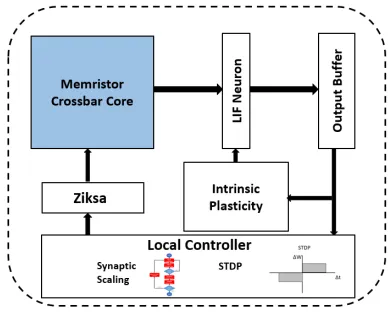
In order to modify the memristors conductance, peripheral circuitry is needed
with the crossbar which is capable of driving a desired potential across the device
which causes a change in the memristors state. In [62] the authors investigate
on-device learning for gradient descent using digital read/write logic with a 2T1R (two
transistors, one memristor) crossbar array. This approach is capable of implementing
fast on-device training at the cost of crossbar area because only two write cycles are
needed, one for increasing the memristance and one for decreasing the memristance.
Another approach is being investigated by Sandia National Laboratories to enable
on-chip back-propagation [61]. In this work an area efficient approach to on-device
training is implemented using Ziksa [34]. Ziksa is a five transistor analog write scheme
for on-device learning with memristor crossbar arrays. The transistors form an
H-bridge across every memristor device as shown in Figure 2.10. With the H-H-bridge, it
is possible to drive a potential across the memristor in either direction represented
by the red and green arrows respectively. The design takes advantage of the power
rails to supply the magnitude of the write pulse and the duration of the pulse controls
the corresponding change in the memristance. The transistors that make up the
H-bridge are controlled by a digital logic block which sequentially writes every column
of memristors one at a time. Every column requires two write cycles, one for positive
writes and another for negative writes. The columns and devices that are not meant to
be trained are driven with a potential which is equal to half the memristors threshold.
The advantages of this design is the scalability because the number of transistors
required grows linearly with the number of rows/columns. Table 2.1 summarizes
Architecture # Devices / Synapse
# Device for 10x10 array
Comments
Ziksa [34] 2/output and 3/input
50 transistors + 100 memristors
Scales with rows and columns
[62] 2 200 transistors
+ 100 memris-tors
Scales with num-ber of synapses
[63] 5 500 transistors
+ 100 memris-tors
[image:39.612.253.395.290.410.2]Design not in context of cross-bar
Table 2.1: Comparison of scalability between Ziksa and other NMS write schemes.
on-device learning implementations. For a more detailed study on Ziksa refer to [34].
Figure 2.10: Ziksa being used to set/reset a memristor in a crossbar setting.
2.3.3 Noise
When designing neuromemristive systems, it is important to account for noise and
variability in the memristive device. Specifically there are two types of noise to take
into consideration, write noise and read noise.
Write noise is primarily due to device variability and will manifest itself in a
few ways. The first manifestation can be seen where an array of similar devices
will have different maximum and minimum resistance states which will impact the
range of synaptic strength a particular device can realize [64, 65, 66, 67]. Second
means that a write pulse with a fixed magnitude and duration cannot be associated
with a fixed conductance change. Thereby updating the conductance by the exact
amount is challenging and often requires the need of extra circuitry which continues
to apply small write operations until the target state is reached [68]. Lastly, two
devices starting from the same initial state will have different conductance changes
when performing an identical write operation [69]. This is due to device variability
and is addressed through using feedback to continue modifying the memristor until
it reaches the target state.
Read noise in the memristor device is due to thermal noise, flicker noise, and
random telegraph noise (RTN) [70, 71, 72, 73, 74, 75]. RTN is the dominating noise
source [70] in these devices and is caused by single electron trapping processes which
cause the device to oscillate between two states. This form of noise can be modelled
through a Gaussian distribution [70].
2.4
Summary
The LSM is a form of RC computing which has distinct properties making it
suit-able for hardware implementations compared to other RC networks when considering
area/power constraints and complexity. The networks reduced complexity compared
to other RNN implementations such as LSTM and reduced precision make it an ideal
architecture for embedded platforms. This could lead to a new generation of
neu-romorphic chips for embedded platforms for applications in a variety of fields such
as personal health care, natural language processing, IoT, and autonomous systems.
This work investigates several architectural advancements to potentially improve and
stabilize performance of using the LSM on real-world applications to achieve
state-of-art results. This is an important step in bringing these networks closer to deployment
in industry. The new architecture is presented in the context of a mixed-signal
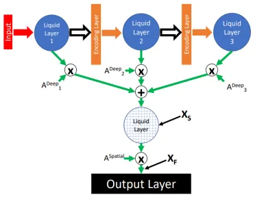
Proposed deep-LSM Architecture
The proposed deep-LSM is a deep network which utilizes random liquid layers as the
main computational unit shown in Figure 3.1. The deep-LSM utilizes random liquid
layers to process temporal information with minimum complexity. In between the
random liquid layers, encoding layers are used to transform the liquid layers state
into a low-dimensional and meaningful representation. As information flows through
the deep-LSM, the different liquid layers will process information from the input
signal over multiple time-scales. The two primary focuses of this research are how
to optimize the random liquid layers for on-device learning and how to best encode
information between the liquid layers in the deep-LSM. The optimized liquid layer
was then tested in several deep architectures described in the second half of this
chapter.
3.1
Liquid Layer Optimization
The LSM architecture consists of a three layer neural network comprised of an input
layer, a liquid layer, and a readout layer as shown previously in Figure 2.1. The input
layer and liquid layer are first simplified to reduce design complexity without any cost
in the performance of the LSM. A simplified short-term plasticity rule and synaptic
scaling are introduced in the liquid layer to help improve the memory and temporal
processing capabilities of the liquid layer which is the primary computational unit in
the deep-LSM.
The input layer in this case is treated as a layer of linear neurons with the identity
function. In this case spiking stimuli to the network is directly passed as spike trains
into the LSM while analog signals are directly fed as current signals to the LSM.
This removes the need for a preliminary conversion layer which translates the analog
signals into spike trains. The connectivity matrix from the input layer to the LSM is
also simplified to a sparse binary matrix. This reduces the precision and complexity of
generating the input weights. The probability of a connection is drawn from a uniform
random distribution and the degree of sparsity varies based on the application and
number of input signals. Figure 3.2 shows an example of the connection from an
input layer with ten features to a 10x10 reservoir of neurons with 95% sparsity. The
sparsity constraint results in mixed-selectivity in the network in which neurons in the
reservoir receive small unique combinations of the input signals. This lets different
neurons respond to different features in the input space without the need for learning
selective response. In [76] the authors explore the trade-offs of mixed selectivity in
random networks and show that there is a trade-off between the degree of separability
and the generalization capability of the network. The appropriate degree of sparsity
is application dependent and needs to be explored as a hyper-parameter for different
Figure 3.2: Sparse projection from the input layer to the liquid layer.
Figure 3.3: Sparse connectivity of a 10x10 liquid layer using (2.3) with λ= 4.
The liquid layer in this work is implemented by leaky integrate-and-fire neurons
whose dynamics are modeled by (2.1). The connections between each neuron are
initialized according to the probability equation (2.3). The resulting small world
topology for a 10x10 grid of spiking neurons is shown in Figure 3.3 where it can be
seen that a few neurons act as hubs which communicate with their local neighbors..
This matrix is initialized using fixed weights for each connection type where excitatory
to excitatory (EE) connections have a synaptic strength of 3, EI have a strength of
3, IE have a strength of 4, and II have a strength of 1 [16]. In [77] it was shown that
neurons having homogeneous excitability is important in the dynamics of working
inhibitory pre-synaptic connections are normalized so the sum of excitatory synapses
and sum of inhibitory synapses is consistent for all neurons. However, the ratio
between the sum of excitatory synapses to the sum of inhibitory synapses is crucial
for information transfer in the brain at the level of individual neurons [78]. It was
found through analysis on the synthetic application that for the proposed LSM, the
best ratio was for the sum of the excitatory synapses to be twice the sum of the
inhibitory synapses. Another simplification is to reduce the STP equations ((2.5)
and (2.6)) to (3.1) as shown in Figure 3.4
S(n) =S(n−1)−α∗(x(n)−β) (3.1)
Figure 3.4: Comparison of STP model in [2] to the proposed STP model.
where S is the synaptic efficacy regulating the strength of a neurons action potential
and is bounded between 0 and 1. If a neuron emits a spike (x(n) = 1), the strength
of S is decreased and if x(n) = 0 then S is increased. α and β are hyper-parameters
used to control the dynamics of STP. STP has also been shown to play a role in
working memory in networks of excitatory and inhibitory neurons. Figure 3.5 shows
the dynamics of the synaptic efficacy S.
Figure 3.5: STP model according to (3.1) as a function of the pre-synaptic action poten-tials with α= 0.01 and β= 0.3.
function. However, because a binary state matrix is used to represent the liquid layers
activity, several states collapse upon each other which can impact the networks ability
to distinguish between different temporal patterns. Typically an exponential filtering
operation is performed on the output of each neuron in the liquid layer [79], in this
work a synaptic trace operation is implemented at the output of each liquid neuron
before transmitting to the readout layer. This operation is given by equation (3.2)
τtrace
dXtrace
dn =−Xtrace (3.2)
where the synaptic trace (Xtrace) keeps track of the behavior of the spike activity of
a neuron (x(n)) by increasing the trace by one every time a spike occurs and slowly
decaying. This trace value is used by the readout layer to perform classification and
prediction by capturing the short term behavior of each liquid neuron. This provides
more information than a binary vector representing if a liquid neuron spiked.
3.2
Clockwork-LSM
One essential property needed for processing temporal information is the ability to
ex-tract information on multiple timescales. Such a feature captures information fed into
the network at different frequencies, resulting in more complex dynamics which should
net-However, as shown in the clockwork-RNN [45], it is beneficial to process information
at different frequencies more distinctly. To capture this in the LSM, a proposed
ap-proach is to give the liquid neurons different firing thresholds and time constants.
This will result in each neuron integrating information over different timescales and
can increase the complexity of network dynamics. In order to keep the initialization
as simple as possible, the number of possible values for the firing threshold and
time-constant are limited in this work. For the firing threshold the neurons can have either
20mV or 40 mV and for the time-constant the neuron can have 30, 60, 90, or 120.
These ranges were found to work best on the synthetic dataset.
A network of heterogeneous neurons enables diversity in the network response and
some neurons will be capable of capturing information on shorter time-scales which
others cannot and vice-versa. This can be seen in Figure 3.6 where neurons with
longer time-constants/higher thresholds will react to changes in the input signal over
longer time-scales while neurons with short time-constants/small thresholds will react
to changes in the input over shorter time-scales. However, as will be shown later, it
will be difficult to implement neurons with different time-constants and thresholds in
the analog domain.
3.3
deep-LSM
The second focus in this work is the implementation of a deep-LSM. In [46], the
au-thors summarize three main areas for optimizing learning algorithms which are; the
number of computations required during training and testing, number of examples
required for good generalization, and minimum amount of human effort needed to
tailor the algorithm to a task. The authors provide evidence showing for many tasks,
a deep network is computationally more efficient than a shallow (single-layer)
archi-tecture. Second, a deep model allows the network to learn more complex abstractions
of the input and process the input on different timescales [46]. Through this process
a network can extract higher level temporal features in each subsequent liquid layer
before finally sending the information to a readout layer.
The inputs to each layer in the deep-LSM can be described by equations (3.3)-(3.5)
IL1(n) = WinL1 ∗u(n) +W L1
rec∗xL1(n−1) (3.3)
IEk(n) =W
Ek
in ∗xEl=k(n) (3.4)
ILl(n) =W
Ll
in ∗xEk=l−1(n) +W Ll
rec∗xLl(n−1) (3.5)
where (3.3) is the input to the first liquid layer L1, (3.4) is the input to the kth
encoding layer, and (3.5) is the input to the deep liquid layers. In this architecture
there is always one more liquid layer than encoding layers.
Two architectures are investigated in this work to realize the deep-LSM. The
first architecture uses fixed (not-trained) encoding layers between different reservoir
layers (liquid layers) which is referred to as the feed-forward deep-LSM. The second
and is referred to as the unsupervised deep-LSM.
3.3.1 Feedforward deep-LSM
The firs architecture investigated is the feedforward deep-LSM. In the feed-forward
deep-LSM, the first step is to identify a group of backbone neurons similar to [43].
These backbone neurons are the neurons responsible for receiving incoming stimuli
and communicating with sequential layers. The location of the backbone neurons is
kept constant throughout all the layers. In this architecture, as shown in Figure 3.7,
the input layer is randomly projected to the backbone neurons in the first liquid layer.
[image:48.612.235.420.325.465.2]There are several approaches to building a deep-LSM from the first layer.
Figure 3.7: A percentage of neurons in the liquid layer are randomly selected as backbone neurons. In the proposed deep-LSM models, the sequential liquid layers are all the same size and the backbone neurons are the same in each liquid.
The first approach is a direct feedforward connection between corresponding
back-bone neurons in sequential layers as shown in Figure 3.8 forming a chain of liquid
layers. The backbone neurons will capture information about the dynamics of the
input signal from the input being directly sent to the reservoir and the feedback
information in the recurrent connections. This information is encoded in the firing
patterns of the backbone neurons which will be sent the next liquid layer. In each
connections and corresponding signals from the previous layer. This lets each
sequen-tial layer build upon the dynamic information from the previous layer and project it
into a new high-dimensional space.
Figure 3.8: Architecture for a deep-LSM consisting of a chain of liquid layers.
The second approach is to use a intermediary feedforward layer of spiking neurons
as shown in Figure 3.9 where the number of neurons in the feedforward layer are equal
to the number of backbone neurons in the liquid. The feedforward layer will receive
a random combination of inputs from the backbone neurons of the first layer and
project them to one backbone neuron in the second layer. Another approach shown
in Figure 3.10 is where the feedforward layer randomly connects to the backbone
neurons in the second layer. The idea behind these two approaches is to take a
non-linear transformation of the input of the previous liquid layers to drive the second
liquid layer.
These approaches do not scale as the reservoir size grows because the number of
backbone neurons will increase dramatically. For a liquid size of 500 neurons, if each
input signal connects to 5% of the neurons in the liquid there will be on average
350 backbone neurons. An approach to circumvent this problem is to use a form of
spike based pooling between the liquid layers as shown in Figure 3.11. The pooling
operation will observe the activity of locally connected groups of neurons formed
Figure 3.9: Architecture for a deep-LSM consisting of an intermediary feedforward net-work with a direct one-to-one connection to the next liquid layer.
Figure 3.10: Architecture for a deep-LSM consisting of an intermediary feedforward net-work randomly connected to the next liquid layer.
spiking output of the pooling layer will then project randomly into the backbone
neurons of the next liquid layer. This approach reduces the number of input signals
to the sequential liquid layers which will minimize the resources needed to implement
the next liquid layer for on-device plasticity.
3.3.2 Unsupervised deep-LSM
The second architecture investigated in this work uses pooling and unsupervised
learn-ing to extract meanlearn-ingful features from each liquid layer. There are two separate
models investigated for this approach. The first model performs unsupervised
learn-ing directly on the outputs of the backbone neurons in the first liquid layer as shown
Figure 3.11: Architecture for a deep-LSM consisting of an intermediary feedforward pool-ing layer randomly connected to the next liquid layer.
neurons in the next liquid.
Figure 3.12: Architecture for a deep-LSM consisting of an intermediary feedforward unsu-pervised layer randomly connected to the next liquid layer (Dashed lines represent trained synapses).
The second model shown in Figure 3.13 utilizes a pooling layer to group the
activi-ties of the backbone neurons and reduce the number of signals which the unsupervised
layer will need to learn. The pooling layer is used to reduce the dimensionality of the
liquid layers output as well as make it translation invariant. This architecture can
simplify the unsupervised implementation to enable on-device learning. Same as in
the previous model, the unsupervised layer will then connect randomly to the neurons
in the next liquid layer.
The motivation behind these two models is that the unsupervised layer can learn
mean-Figure 3.13: Architecture for a deep-LSM consisting of an intermediary feedforward unsu-pervised pooling layer randomly connected to the next liquid layer (Dashed lines represent trained synapses).
ingful information to send the next liquid layer. This helps maximize the information
communicated between layers and gives a better representation of the liquid layer
dynamics than a direct or random propagation of information which may send
redun-dant information [25].
The unsupervised learning rule used is known as Spike-time Dependent Plasticity
(STDP). STDP is a form of hebbian learning which postulates that neurons which
fire together grow together [80]. In this case if a pre-synaptic potential occurs before
a post-synaptic potential the synaptic strength is increased and in the other case if a
post-synaptic potential occurs before a pre-synaptic potential the synaptic strength
is decreased. This can be mathematically represented by
∆Wi,j =
A+∗exp−∆τT, 0≤∆T ≤t max
A−∗exp∆τT, 0>∆T ≥tmin
0, else
(3.6)
where ∆Wi,j is the change in the synaptic strength between a pre and post-s