Theses
10-18-2018
Evolution of A Common Vector Space Approach
to Multi-Modal Problems
Chi Zhang
[email protected]Follow this and additional works at:
https://scholarworks.rit.edu/theses
This Dissertation is brought to you for free and open access by RIT Scholar Works. It has been accepted for inclusion in Theses by an authorized administrator of RIT Scholar Works. For more information, please [email protected].
Recommended Citation
by
Chi Zhang
B.S. Shandong University, 2009
B.S. Jinan University, 2009
M.S. Rochester Institute of Technology, 2013
A dissertation submitted in partial fulfillment of the
requirements for the degree of Doctor of Philosophy
in the Chester F. Carlson Center for Imaging Science
College of Science
Rochester Institute of Technology
October 18, 2018
Signature of the Author
Accepted by
ROCHESTER INSTITUTE OF TECHNOLOGY
ROCHESTER, NEW YORK
CERTIFICATE OF APPROVAL
Ph.D. DEGREE DISSERTATION
The Ph.D. Degree Dissertation of Chi Zhang has been examined and approved by the dissertation committee as satisfactory for the
dissertation required for the Ph.D. degree in Imaging Science
Dr. Carl Salvaggio, Dissertation Advisor Date
Coordinator Ph.D. Degree Program Date
Dr. Pengcheng Shi Date
Dr. Raymond Ptucha Date
Dr. Alexander Loui Date
COLLEGE OF SCIENCE
CHESTER F. CARLSON CENTER FOR IMAGING SCIENCE
Title of Dissertation:
Evolution of A Common Vector Space Approach to Multi-Modal Problems
I, Chi Zhang, hereby grant permission to Wallace Memorial Library of R.I.T.
to reproduce my thesis in whole or in part. Any reproduction will not be for
commercial use or profit.
Signature
Date
1 Introduction 19
2 Spatio-Temporal Video Segmentation 28
2.1 Related Work . . . 29
2.2 System Framework and Algorithms . . . 33
2.2.1 Points Tracking . . . 34
2.2.2 Motion Clustering . . . 37
2.2.3 Supervoxel Clustering . . . 42
2.2.4 Coarse Segmentation . . . 45
2.2.5 Graph-based Fine Segmentation . . . 46
2.3 Experimental Results . . . 48
2.3.1 Parameters Settings . . . 48
2.3.2 Evaluation on SegTrack Dataset . . . 49
2.3.3 Evaluation on Kodak Alaris Consumer Video Dataset . . . 53
2.4 Discussion . . . 56
3 Batch-Normalized Recurrent Highway Networks 58 3.1 Related Work . . . 59
3.2 Developed Framework . . . 60
3.3 Experimental Results . . . 63
3.3.1 Experimental Setup . . . 63
3.3.2 Image Captioning Results . . . 65
3.4 Discussion . . . 69
4 Semantic Sentence Embeddings 70 4.1 Related Work . . . 71
4.2 Methodology . . . 72
4.2.1 Vector Representation of Sentences . . . 72
4.2.2 Hierarchical Encoder for Text Summarization . . . 75
4.3 Experimental Results . . . 77
4.3.1 Datasets . . . 77
4.3.2 Training Details . . . 78
4.3.3 Sentence Paraphrasing . . . 79
4.3.4 Text Summarization . . . 80
4.4 Discussion . . . 81
5 Multi-Modal Vector Representation 83 5.1 Related Work . . . 86
5.2 Methodology . . . 88
5.2.1 Multi-Modal Vector Representation . . . 88
5.2.2 n-gram Metric Conditioning . . . 90
5.2.3 Conditioning on Multiple Captions . . . 90
5.2.4 MMVR Architecture . . . 91
5.3 Results and Discussion . . . 93
5.3.1 Inference . . . 93
5.3.2 Evaluation Metrics . . . 94
5.3.3 Text-to-Visual . . . 95
5.3.4 Text Generation . . . 99
6 Conclusions and Future Work 104
6.1 Conclusions . . . 104
6.2 Future Work . . . 107
6.2.1 Common Vector Space . . . 108
6.2.2 Losses for Metric Learning . . . 109
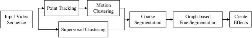
2.1 The overall coarse-to-fine framework for video segmentation and
recom-position. . . 33
2.2 KLT point tracking. (a) Selected tracking points in the 1st frame; (b)
and (c) Tracking points in the 3rd and 5th frame. . . 37
2.3 Demonstrations of point trajectory clustering using SSC algorithm on two
frames. The yellow and red markers represent two clusters, foreground
and background respectively. . . 41
2.4 Initialization and the search region of the supervoxel. Red box shows
the initialized supervoxel along D consecutive frames. Blue box is the
searching area for this cluster. Each pixel is calculated eight times since
it enclosed by eight cluster search region. . . 44
2.5 Results of 3D SLIC voxel grouping on three consecutive frames. The
boundaries of each supervoxel are shown in yellow. The block enclosed
by the yellow boundaries in the corresponding position between frames
has the same label. . . 45
2.6 Coarse segmentation by combining the results of SSC and 3D SLIC
algo-rithms. (a) Tracking points generated by KLT and SSC. The yellow and
red markers represent the foreground and background region respectively;
(b) The 3D SLIC supervoxels on the same frame; and (c) The mask
gener-ated by combining (a) and (b). The black, gray and white regions denote
determined background, undetermined region and determined foreground
respectively. . . 46
2.7 Result of fine segmentation using GrabCut method. (a) The algorithm
segment the undetermined region to light and dark gray regions; and
(b) The light and dark gray regions are merged to the background and
foreground respectively to form the final mask. . . 47
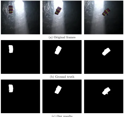
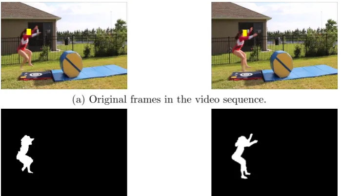
2.8 Qualitative results of SegTrack “parachute” video sequence. . . 51
2.9 Qualitative results of SegTrack “girl” video sequence. . . 52
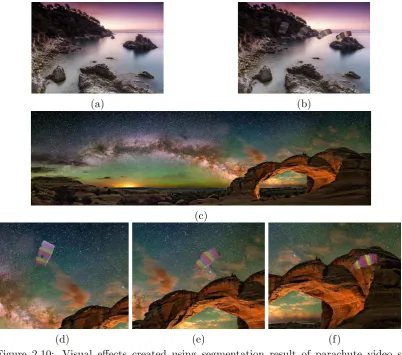
2.10 Visual effects created using segmentation result of parachute video
se-quence. (a) The background used to create static effect in (b); (b) A static
image synthesized by the segmentation result and (a); (c) A panorama
used to create dynamic effects as shown in (d) to (f); and (d) to (f) The
video frames generated by synthesizing the segmentation result and (c). 53
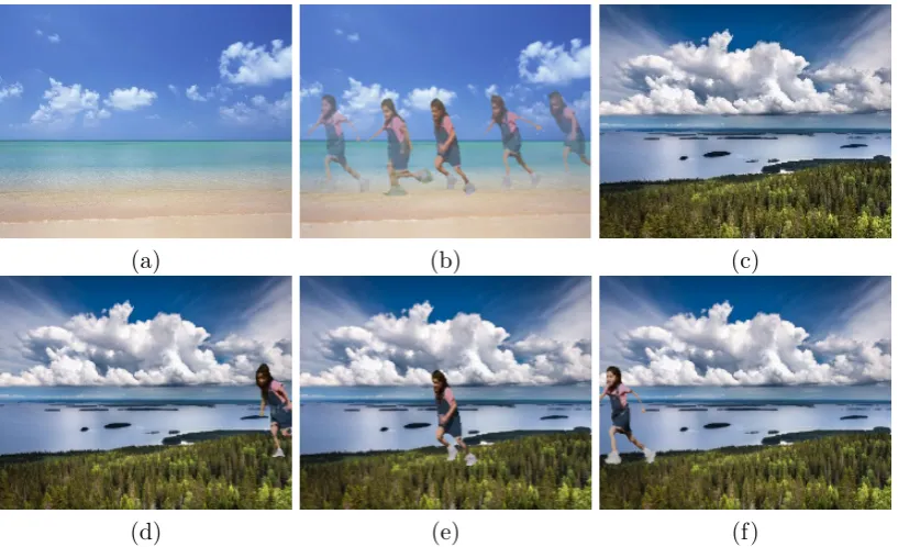
2.11 Visual effects created using segmentation result of girl video sequence.
(a) The background used to create static effect in (b); (b) A static image
synthesized by the segmentation result and (a); (c) The background used
to create dynamic effect in (d) to (f); and (d) to (f) The video frames
generated by synthesizing the segmentation result and (c). . . 54
2.12 Object segmentation results on “gymnast1” video sequence in Kodak
Alaris consumer video dataset. . . 55
2.13 Object segmentation results on “dog” video sequence in Kodak Alaris
3.1 The architecture of batch normalized recurrent neural networks. T and C
denote transform and carry gates specified in (3.2) and (3.3) respectively,
H is a nonlinear transform specified by (3.1), and BN represents batch
normalization operation. . . 62
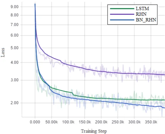
3.2 The total loss change vs. training steps. All dark curves are smoothed
by a factor of 0.8. The light curves are not smoothed. . . 66
3.3 Example results on MSCOCO captioning dataset. . . 67
3.4 More results on MSCOCO captioning dataset. The bottom two are
neg-ative examples. . . 68
4.1 The typical image-to-text (image captioning) inference model. The CNN
encodes the image into a feature vector h, which is decoded by the
fol-lowing RNN. . . 70
4.2 The sentence paraphrasing model. The red and blue cells represent
en-coder and deen-coder respectively. The intermediate vector in black (sent2vec)
is vector encoded sentence. . . 73
4.3 The paragraph summarizer. The red and blue cells represent encoder and
decoder respectively. The encoder inputsxi are the vector representation
generated using sent2vec of the sentences in the paragraph. The decoder
outputs yi are the words in summarized text. The intermediate vector
in black (paragraph2vec) is vector encoded paragraph. Dashed arrows
indicate temporal boundaries. . . 76
4.4 Some paraphrase sentence pairs are represented by the sent2vec and then
projected into 2D space using PCA. Each point represents a sentence in
SICK dataset and the corresponding sentence is shown on the right. . . 80
4.5 t-SNE visualizations of single sentence descriptions of a subset of all
se-quences on TACoS Multi-Level Corpus. (a) The developed sent2vec; (b)
Skip-thoughts and (c) Skip-gram. Points are colored based on their
5.1 Different types of multimedia are semantically connected to each other
by a common vector space (CVS). . . 84
5.2 High level view of image-to-text conversion using CVS. . . 84
5.3 Overview of the bidirectional image-text generation model. To form the
respective encoder and decoder networks, a CNN-GAN combination is
used for visual and a recurrent machine translation model for text
modal-ities. . . 85
5.4 Overview of the MMVR model. It consists of two pre-trained modules –
an image generator (G) that inputs a latent representation ht and
gen-erates an image ˆx; and an image captioner that inputs an image ˆx and
generates a caption ˆy. To update the latent vector ht, cross-entropy
be-tween the generated caption ˆyand a ground truth captiony is used while
the weights for the generator and CNN are fixed. . . 88
5.5 Conditioning the image generation through multiple captions by
aggre-gating the gradients from individual caption cross-entropy. Solid black
lines show the direction of forward pass during sentence generation and
dashed red lines show direction of error back-propagation during latent
vector update. . . 91
5.6 Examples of the YOLO object detection on generated images. The
bound-ing boxes and correspondbound-ing labels are detections with confidence greater
than 0.5 threshold. . . 95
5.7 Examples of text-to-visual transformation. . . 96
5.8 Examples of the text-to-image generation as conditioned on varying
num-ber of input captions. One can observe more detailed images being
syn-thesized with increase in captions. . . 97
5.9 Examples comparing the text-to-image for PPGN and the BLEU-1 scaled
cross-entropy. Even though slight improvements could be observed with
5.10 Examples that show text-to-image improvements after fine-tuning the
generator on MS-COCO dataset. Object categories such as giraffe and
stop sign that are not part of ImageNet dataset show some enhancement in details. One can also observed slight improvements in understanding
of size, shape and quantity aspects. . . 100
5.11 Examples of the visual-to-text (left) and text-to-text (right) modes of the MMVR. The inputs can be the visual or text modalities. . . 101
5.12 Examples of arithmetic operations in the latent space for the text-to-text model. . . 102
6.1 The CVS model training architecture. The solid arrows and dashed ar-rows represent image path and text path respectively, the dotted line indicates the connection to CVS. . . 109
6.2 Triplet loss on two positive examples and one negative example. . . 110
6.3 The three types of negatives, given an anchor and a positive. . . 112
2.1 Quantitative pixel-level errors and comparison with the state-of-the-art
methods on SegTrack dataset. . . 50
3.1 Evaluation metrics on MSCOCO dataset. LSTM: regular RNN model
with LSTM cell; RHN: model with original RHN cell; BN RHN: the
developed model with RHN constrain relaxed and batch normalization
applied instead. . . 64
4.1 Sentence pairs statistics in captioning datasets. . . 77
4.2 Test set results on the SICK semantic relatedness task, where 300, 1024
denote the number of hidden units and 20k, 50k denote the size of the
vocabulary. r and ρ are Pearson’s and Spearman’s metric respectively. . 79
4.3 Evaluation of short to single sentence summarization on TACoS
Multi-Level Corpus using vectors from sent2vec, skip-thoughts, and skip-gram
respectively. . . 80
5.1 Evaluation of the generated image quality using the inception, detection
and human scores on the test set. . . 96
5.2 Evaluation of the generated image quality by conditioning on varying
number of paraphrased sentences (NC). . . 97
5.3 Comparison of image quality with different BLEU metrics for scaling the
latent vector update function. . . 99
5.4 Evaluation of Text-to-Text paraphrasing model with variation of noise in
the latent vector space. The noise scale is the multiplier for the standard
deviation of the feature space to generate random uniform noise. Noise
by
Chi Zhang
Submitted to the
Chester F. Carlson Center for Imaging Science in partial fulfillment of the requirements
for the Doctor of Philosophy Degree at the Rochester Institute of Technology
Abstract
A set of methods to address computer vision problems has been developed. Video
un-derstanding is an activate area of research in recent years. If one can accurately identify
salient objects in a video sequence, these components can be used in information retrieval
and scene analysis. This research started with the development of a course-to-fine
frame-work to extract salient objects in video sequences. Previous frame-work on image and video
frame background modeling involved methods that ranged from simple and efficient to
accurate but computationally complex. It will be shown in this research that the novel
approach to implement object extraction is efficient and effective that outperforms the
existing state-of-the-art methods. However, the drawback to this method is the inability
to deal with non-rigid motion.
With the rapid development of artificial neural networks, deep learning approaches
are explored as a solution to computer vision problems in general. Focusing on image
and text, the image (or video frame) understanding can be achieved using CVS. With
this concept, modality generation and other relevant applications such as automatic
im-age description, text paraphrasing, can be explored. Specifically, video sequences can
be modeled by Recurrent Neural Networks (RNN), the greater depth of the RNN leads
to smaller error, but that makes the gradient in the network unstable during training.
To overcome this problem, a Batch-Normalized Recurrent Highway Network (BNRHN)
was developed and tested on the image captioning (image-to-text) task. In BNRHN, the
highway layers are incorporated with batch normalization which diminish the gradient
vanishing and exploding problem. In addition, a sentence to vector encoding framework
that is suitable for advanced natural language processing is developed. This semantic
text embedding makes use of the encoder-decoder model which is trained on sentence
paraphrase pairs (text-to-text). With this scheme, the latent representation of the text
is shown to encode sentences with common semantic information with similar vector
rep-resentations. In addition to image-to-text and text-to-text, an image generation model
is developed to generate image from text (text-to-image) or another image
(image-to-image) based on the semantics of the content. The developed model, which refers to the
Multi-Modal Vector Representation (MMVR), builds and encodes different modalities
into a common vector space that achieve the goal of keeping semantics and conversion
between text and image bidirectional. The concept of CVS is introduced in this research
to deal with multi-modal conversion problems. In theory, this method works not only
on text and image, but also can be generalized to other modalities, such as video and
audio. The characteristics and performance are supported by both theoretical analysis
and experimental results. Interestingly, the MMVR model is one of the many possible
ways to build CVS. In the final stages of this research, a simple and straightforward
framework to build CVS, which is considered as an alternative to the MMVR model, is
I would like to extend my heartfelt thanks to the many people, in many places, who so
generously contributed to the work presented in this thesis.
Special mention goes to my enthusiastic advisor, Dr. Carl Salvaggio for his
funda-mental role in my doctoral work. Carl provided me with every bit of guidance, assistance,
and expertise that I needed during my first few semesters; then, when I felt ready to
venture into research on my own and branch out into new research areas, Carl gave me
the freedom to do whatever I wanted, at the same time continuing to contribute valuable
feedback, advice, and encouragement. I quite simply cannot imagine a better advisor.
Similarly, profound gratitude goes to Dr. Raymond Ptucha, who has been a truly
dedicated mentor. I am particularly indebted to Raymond for his constant faith in my
lab work. I thank Raymond wholeheartedly, not only for his tremendous academic
sup-port, advice, and encouragement, but also for making my Ph.D. an amazing experience.
In addition to our academic collaboration, I greatly value the close personal rapport
that Raymond and I have forged over the years.
I am also hugely appreciative to Dr. Alexander Loui, especially for sharing his
imaging expertise so willingly, and for being so dedicated to his role as my supervisor
during my internship at Kodak Alaris.
I would like to thank the faculties in Chester F. Carlson Center for Imaging Science
at the Rochester Institute of Technology, especially Dr. Derek Walvoord, Dr. Harvey
Dhody, Dr. Roger Easton and Dr. John Kerekes, for the substantial influence that their
courses have had on my research. I gratefully acknowledge the members of my Ph.D.
committee for their time and valuable feedback on a preliminary version of this thesis.
Special mention goes to Shagan Sah, Thang Nguyen, Dheeraj Kumar Peri, Ameya
Shringi, Dr. John Hamilton, Dr. Nathan Cahill, and all students in MIL lab who
contributed to the work presented in this thesis, for for their infinite patience and our
fruitful collaboration there. Among many other things, I am thankful to Jim Bodie and
Brett Matzke, for providing me with a fantastic hardware and software support. And
to Elizabeth Lockwood, Susan Chan and Joyce French, for handling logistics efficiently
and effectively.
Finally, but by no means least, thanks go to my mum and dad for almost unbelievable
support, love, and sacrifices. Without them, this thesis would never have been written.
They are the most important people in my world and I dedicate this thesis to them.
This last word of acknowledgment I have saved for my beloved girlfriend, Meng Wang,
Introduction
This research will start from the general area of multimedia analysis, especially on video
background modeling, object extraction and video text summarization. With the rapid
development and lower cost of smartphones and new digital capture devices, consumer
videos are becoming ever popular as is evident by the large volume of YouTube video
uploads, as well as video viewing on the Facebook social network. These large amount
of videos pose a great challenge for users to organize, access, and retrieve their content.
Hence, the ability to efficiently analyze, index, and summarize consumer videos will
en-able fast retrieval and intelligent re-purposing of video content for advanced and novel
consumer imaging applications. This research will develop and validate a unified video
analysis framework for automatically processing, analyzing, segmenting, and
summa-rizing unstructured and unrestricted user-generated videos in the wild. In addition to
multimedia analysis, this research is also concerned with the interaction between them,
especially on text and image (video frame), using learning approaches. In recent years,
deep learning has improved performance on many vision and language tasks
individ-ually. However, general vision or language models cannot emerge within a paradigm
that focuses on the particularities of a single metric, dataset, and task. Deep learning
has enabled dramatic advancement in image, video and text understanding. For
exam-ple, image classification, object detection, image captioning, localized image description,
image and sentence retrieval and visual question answering tasks have witnessed
tremen-dous progress in the past few years. A unified Common Vector Space (CVS) for vision
and language will be introduced in this research, which encodes different sources (not
limited to image and text) by a latent vector space, where similar inputs from different
modalities cluster together and dissimilar ones separate. It is expected that the
combi-nation of these resources will facilitate research in multitask learning, transfer learning,
general embeddings and encoders, architecture search, zero-shot learning, general
pur-pose question answering, meta-learning, and other related areas of vision and language.
Object level video segments are semantically meaningful spatio-temporal units such
as moving people, moving vehicles, a flowing river, etc. Segmentation of a video sequence
into a number of component regions would benefit many higher level vision based
appli-cations such as scene analysis, object localization and content understanding. However,
single target object extraction would be a more demanding task considering consumers’
needs. In many cases, a consumer video sequence simply targets capturing a single
object’s movement in a specific environment such as dancing, skiing, running, etc. In
general, motion object detection and extraction for a static video camera is relatively
straightforward since the background barely changes and a simple frame differencing
would be able to extract a moving foreground object. However, it is still challenging for
the object moving on a cluttered and/or dynamic background.
The goal of background modeling and foreground object extraction is to build a
model of the background/foreground in an offline manner and extract the object of
in-terest by comparing the estimated model with the frames. The model must be robust
enough to cope with background changes in different ways. In recent years, a trend
towards modeling spatio-temporal uniform (in terms of either appearance or motion)
regions instead of single pixels has been observed [1]. These works rely on
superpix-els/supervoxels for object segmentation in videos. However, these methods are
compu-tationally expensive and group superpixels together according to pure spatio-temporal
et al. [2] proposed an approach without making any specific assumptions about the videos that relies on how objects are perceived by humans according to Gestalt laws.
Khorevaet al. [3] proposed an empirical approach to learn both the edge topology and
weights of the graph. The most confident edges are selected by the graph structure while
the classifiers are learned to combine features and seamlessly integrated by its accuracy.
In [4] and [5], Fast Point Feature Histograms (FPFH) and Histogram of Oriented
Gra-dients (HoG) have been used as features to represent superpixels. The high dimension
feature space slows down the computation, although some improvements (e.g., [6]) were
proposed to provide a better balance of trade off between segmentation quality and run
time.
Much research has been devoted to graph models for segmentation, such as [3] and
[7]. Fan and Loui [8] proposed a graph-based approach that models the data in a
feature space, which emphasizes the correlation between similar pixels while reducing
the inter-class connectivity between different objects. In [9], a reduced superpixel graph
was re-weighted such that the resulting segmentation was equivalent to the full graph
under certain assumptions. However, these approaches still suffer from the expense of
computation and low accuracy.
Chapter 2 will investigate inter-relationship between statistical learning, segment or
pixel-level classification and fine segmentation on salient objects in the video sequence.
The research can be used for other applications based on the developed framework, such
as video content retrieval, visual effects generation, video highlight or summarization,
and video content understanding, etc. Chapter 2 first develops a novel coarse-to-fine
framework and prototype system for automatically segmenting a video sequence and
extracting a salient moving object from it. The developed framework is comprised of
point tracking and motion clustering of pixels into groups. In parallel, a pixel
group-ing method is used to generate supervoxels for the correspondgroup-ing frames of the video
sequence. Coarse segmentation is achieved by combining the results of previous steps.
extrac-tion of the salient object.
In addition, recent progress in deep learning using Convolutional Neural Networks
(CNNs) has achieved remarkable performance on various computer vision and pattern
recognition tasks, including video analysis. A video can be considered as a sequence
of frames and the adjacent frames are related by consistent motion and pixel similarity
in terms of pixel color and location. Therefore, video sequences can be modeled by
Recurrent Neural Networks (RNNs). Typically, increasing the depth of the networks
significantly reduces the error on competitive benchmarks [10]. However, training very
deep networks is challenging due to the fact that the distribution of each layer’s inputs
changes during training. When training RNNs, gradients are unstable, and can vanish
or explode over time. In some cases the gradients can vanish, the forward flow often
diminishes, and the training time can be unbearably slow by requiring lower learning
rates and careful parameter initialization. Sometimes the gradient gets much larger in
earlier layers, which causes an exploding gradient problem. More generally, it turns
out that the gradient in deep neural networks is unstable, tending to either explode or
vanish in earlier layers. In such deep architectures the vanishing or exploding gradient
problem becomes a key issue.
Several techniques [11, 12, 13] have been proposed to circumvent the vanishing and
exploding gradient problem. Batch normalization [14] addresses the internal covariate
shift problem by normalizing the layer inputs per mini-batch statistics. This speeds up
training by allowing the usage of more aggressive learning rates, creates more stable
models which are not as susceptible to parameter initialization, and has been shown to
minimize vanishing and exploding gradients. While batch normalization has been found
to be very effective for feedforward CNNs, the technique has not been as prevalent on
RNNs. Laurentet al. [15] reported that applying batch normalization to the
input-to-hidden transitions of RNNs leads to faster convergence but does not seem to improve
the generalization performance on sequence modeling tasks. Cooijmanset al. [16] found
and hidden-to-hidden transition, thereby reducing internal covariate shift between time
steps.
In addition to batch normalization, much attention has been paid to controlling
gra-dient behavior by changing the network structure. For instance, networks with
stochas-tic depth [17] enable the seemingly contradictory setup to train short networks and use
deep networks at test time. This approach complements the recent success of residual
networks. It reduces training time substantially and improves the test error significantly
on almost all data sets. Recent evidence also indicates that CNNs could benefit from
an interface to explicitly construct memory mechanisms interacting with a CNN feature
processing hierarchy. Correspondingly, the convolutional residual memory network [18]
was proposed as a memory mechanism which enhances CNN architecture based on
aug-menting convolutional residual networks with a Long Short-Term Memory (LSTM) [11]
mechanism. Weight normalization [19] was reported to be better suited for recurrent
models such as LSTMs compared to batch normalization. It improves the conditioning
of the optimization problem and speeds up convergence of stochastic gradient descent
without introducing any dependencies between the examples in a mini-batch.
Simi-larly, layer normalization [20] normalizes across the inputs on a layer-by-layer basis at
each time step. This stabilizes the dynamics of the hidden layers in the network and
accelerates training, without the limitation of being tied to a batched implementation.
Chapter 3 develops a novel recurrent framework based on Recurrent Highway
Net-works (RHNs) for sequence modeling using batch normalization. This chapter explores
the differences of several state-of-the-art techniques in terms of gradient control in data
propagation within recurrent networks and compares the performance between them.
The developed technique relaxes the constraint in RHNs such that they have a better
chance to avoid the gradient from vanishing or exploding by normalizing the recurrent
transition units in highway layers. Since this work is able to deal with applications
with RNN structure, such as captioning, it turns out that this technique can be used in
Exploring the new RNN framework brings about benefits for multimedia conversion,
for example, captioning, which is also known as image-to-text conversion.
Text-to-text conversion also needs to be paid attention by using a sequence-to-sequence model.
Modeling temporal sequences of patterns requires the embedding of each pattern into a
vector space. For example, by passing each frame of a video through a CNN, a sequence
of vectors can be obtained. These vectors are fed into a RNN to form a powerful
descriptor for video annotation [21, 22, 23]. Similar, techniques such as word2vec [24]
and GloVe [25] have been used to form vector representations of words. Using such
embeddings, sentences become a sequence of word vectors. When these vector sequences
are fed into an RNN, it generates a powerful descriptor of a sentence [26].
Given vector representations of a sentence and video, the mapping between these
vector spaces can be solved, forming a connection between visual and textual spaces.
This enables tasks such as captioning, summarizing, and searching of images and video
to become more intuitive for humans. By vectorizing paragraphs [27], similar methods
can be used for richer textual descriptions.
Recent advances at vectorizing sentences represent exact sentences faithfully [28, 27,
29], or pair a current sentence with prior and next sentence [30]. Similar to word2vec
and GloVe map words of similar meaning close to one another, the desired method is to
map sentences of similar meaning close to one another. For example, the sentences “A
man jumped over the stream” and “A person hurdled the creek” have similar meaning
to humans, but are not close in traditional sentence vector representations. Just like the
words flower, rose, and tulip are close in good sentence to vector representations, the
example sentences must lie close in the introduced embedded vector space.
Inspired by the METEOR [31] captioning benchmark which allows substitution of
similar words, it is desired to map similar sentences as close as possible. Both paraphrase
datasets and ground truth captions from multi-human captioning data sets are utilized.
For example, the MS-COCO data set [32] has over 120K images, each with five captions
should convey the same semantic meaning. Chapter 4 presents an encoder-decoder
framework for sentence paraphrases, and generate the vector representation of sentences
from this framework which maps sentences of similar semantic meaning nearby in the
vector encoding space.
The main contributions of this semantic sentence embedding method are 1) the usage
of sentences from widely available image and video captioning data sets to form sentence
paraphrase pairs, whereby these pairs are used to train the encoder-decoder model; 2)
the demonstration of the application of the sentence embeddings for paragraph
summa-rization and sentence paraphrasing, whereby evaluations are performed using metrics,
vector visualizations and qualitative human evaluation; and 3) the extention of the
vectorized sentence approach to a hierarchical architecture, enabling the encoding of
more complex structures such as paragraphs for applications such as text
summariza-tion. Chapter 4 presents the developed encoder-decoder framework for sentence and
paragraph paraphrasing.
Looking at the exploration of the relationship between multimedia and vectors,
it is reasonable to extend the goal of this dissertation to find the common vector
representation for different types of sources. In other words, given a(n) video
se-quence/image/audio/sentence/paragraph, the goal is to extract an embedded vector
containing the semantics of the source, and decode it to any type of the multimedia.
The embedded vectors from different types of sources lie in a common space so that
there is no need to align the vectors in the generative models. As an example, image
captioning converts an image into a vector, and then the vector is used to generate text.
In the other direction, the vector representation should be able to generate an image
with related content. The common vectors form a space referred to as common vector
space (CVS).
For simplicity, the study is focusing on images and text. Specifically, the common
vector space deals with four source-target conversion: text-text (text2text, which can be
as known as image captioning model as illustrated in Chapter 3), text-image (text2im,
as illustrated in Chapter 5), and image-image (im2im, as illustrated in Chapter 5).
Recent success in image captioning [33, 34, 35, 36] has shown that deep networks
are capable of providing apt textual descriptions of visual data. In parallel, advances in
conditioned image generation [37, 38, 39, 40] provide diverse images from a text based
prior. An ambitious goal for machine learning in the vision and language domain is
to be able to represent different modalities of data that have the same meaning with
a common latent representation. For example, words like “baseball” and “batter”, a
sentence describing a baseball game, or image representations of a baseball game all
refer to similar concepts. Generally, concepts that are semantically similar would lie
close together in the descriptor’s space while dissimilar concepts would lie farther apart.
A sufficiently powerful model should be able to store similar concepts in a similar
repre-sentation or produce any of these realizations from the same latent space. Successfully
mapping visual and textual modalities in and out of this latent space would significantly
impact the broad task of information retrieval.
Chapter 5 develops a cross-domain model, based on Plug & Play Generative
Net-works (PPGN) [37] architecture, capable of converting between text and image. The
networks used in these domains are combined by merging the latent representations
obtained during transition. The goal of the latent vector representation is to encourage
similar patches to have descriptors that are closer to each other in the descriptors’ space
than dissimilar ones. The contributions of this model are as follows: 1) The formulation
of a latent representation based model that merges inputs across multiple modalities; 2)
Development of an n-gram based cost function that generalizes better to a text prior;
3) Improvements on image quality while using multiple semantically similar sentences
for conditioning image generation on generalized text; and 4) To advance qualitative
measurement of text-to-visual models, an object detector based metric is introduced,
and the human evaluations are conducted which compare the metric to the standard
In addition to the PPGN based model, the concept of a unified Common Vector Space
(CVS) for vision and language is introduceed, that spans across five broad tasks:
classi-fication, captioning, object detection, retrieval and visual question answering. Chapter
6 first summarizes the work we have done, then introduces the idea of learning a
Com-mon Vector Space (CVS) where similar inputs from different modalities cluster together.
It is expected that the combination of these resources will facilitate research in
multi-task learning, transfer learning, general embeddings and encoders, architecture search,
zero-shot learning, general purpose question answering, meta-learning, and other related
areas of vision and language. The contribution of the CVS model would be: 1)
For-mulating an efficient vector space based model using neural embeddings that act as a
bridge between vision and language modalities and is easily expandable to new
modali-ties; 2) Introducing a multi-modal loss function that includes metric loss, category loss
and adversarial loss terms. The adversarial framework includes within-modality and
across modality discriminators; and 3) It is capable to applying this model to new tasks,
Spatio-Temporal Video
Segmentation
Object level segmentation of the video sequence would benefit many higher level vision
based applications such as scene analysis, object localization and content understanding.
However, single target object extraction would be a more demanding task considering
consumers’ needs. In many cases, a consumer video sequence simply targets
captur-ing a scaptur-ingle object’s movement in a specific environment. In general, it is challengcaptur-ing
for the object moving on a cluttered and/or dynamic background, since simple frame
differencing would not be able to extract a moving foreground object.
The goal of background modeling and foreground object extraction is to build a
model of the background/foreground in an offline manner and extract the object of
interest by comparing the estimated model with the frames. Recently, modeling on
spatio-temporal uniform regions [1] becomes popular approaches. Moreover, researchers
have focused on graph models for segmentation, such as [3] and [7]. However, these
approaches still suffer from the expense of computation and low accuracy.
In this chapter, a discussion that focuses on the coarse-to-fine framework and
pro-totype for automatic video sequence segmentation and salient moving object extraction
are presented. Effectively, voxel grouping techniques are often used to generate
super-voxels for video sequences and describe how similar the adjacent super-voxels are in terms
of appearance and motion. At a top-level, segmentation of video sequences becomes a
problem of classification of supervoxels into foreground or background. With the
seg-mentation results, some interesting and pleasing visual effects can be created easily for
consumers. This is known as video object recomposition.
The developed framework is comprised of point tracking algorithms and motion
clustering of pixels into groups. In parallel, a pixel grouping method is used to generate
supervoxels for the corresponding frames of the video sequence. Coarse segmentation
is achieved by combining the results of previous steps. Subsequently, a graph-based
segmentation technique is used to perform fine segmentation and extraction of the salient
object. Section 2.1 outlines some related work and approaches on video modeling and
moving object segmentation. Section 2.2 first gives an overview of the developed
coarse-to-fine video segmentation framework and the system workflow, and then describes the
details of the key algorithms and components of the developed framework. Section
2.3 discusses the performance evaluations and experimental results of the developed
framework and algorithms. Finally, some discussions and future work are presented in
Section 2.4.
2.1
Related Work
The goal of background modeling and foreground object extraction is to build a model
of the background/foreground in an off-line manner and extract the object of
inter-est by comparing the inter-estimated model with the frames. The model must be robust
enough to cope with background changes in different ways. This section reviews some
of the relevant state-of-the-art methods on video segmentation in terms of the following
aspects:
modeling spatio-temporal uniform (in terms of either appearance or motion) regions
instead of single pixels has been observed. These works rely on superpixels/supervoxels
for object segmentation in videos. The core idea is that in superpixels appearance and
motion are more or less uniform, thus estimated density functions are likely to be quite
accurate. However, these methods 1) need to compute the motion field through optical
flow, which is computationally expensive; 2) group superpixels together according to
pure spatio-temporal similarity (in terms of appearance) without exploiting real-world
object features; and 3) produce segmentation through global minimization of an energy
function, thus considering video object segmentation as a single objective optimization
problem, while, in fact, it is intrinsically multi-objective. As an improvement, Giordano
et al. [2] proposed an approach without making any specific assumptions about the videos and it relies on how objects are perceived by humans according to Gestalt laws.
This methods is able to segment objects in crowded scenes and accurately segments
com-plex articulated objects. From another point of view, meaningful features are necessary
in frame partitions for good video segmentation. Much literature [42, 43] has proposed
features for appearance, motion or shape similarities among the graph nodes. Most
works are currently limited in the number of features they can leverage, as often the
researchers hand-design the feature combination to measure similarity between pixels or
superpixels. Khoreva et al. [3] proposed an empirical approach to learn both the edge
topology and weights of the graph. The most confident edges are selected by the graph
structure while the classifiers are learned to combine features and seamlessly integrated
by its accuracy. In [5] and [4], HoG and FPFH have been used as features to represent
superpixels. The high dimension feature space slows down the computation, although
some improvements (for example, [6]) were proposed to provide a better balance of trade
off between segmentation quality and runtime.
Graph Based Approaches. Much research has been devoted to graph partitioning
models [44, 45]. While measurable differences have been observed, Khoreva et al. [3]
and successful graph partitioning model [7] based on spectral clustering. Fan and Loui [8]
proposed a graph-based approach that effectively models the data in a high-dimensional
feature space, which emphasizes the correlation between similar pixels while reducing the
inter-class connectivity between different objects. The graph model fuses appearance’
spatial and temporal information to break a volumetric video sequence into semantic
spatiotemporal key-segments. In the work of Liet al. [9], the reduced superpixel graph
was reweighted such that the resulting segmentation was equivalent to the full graph
under certain assumptions. Among this type of algorithms, constructing the graph is
a vital step for ensuring the performance of clustering methods. Although graph-based
methods have been extensively studied, there have been limited efforts for building
effective graphs. The most popular method for constructing a sparse graph is the nearest
neighbor approach, including different variants such ask-nearest neighbor and-nearest
neighbor methods.
Learning Based Approaches. Learning based models consist one of the major
themes in image and video segmentation. They learn the appearance of semantic
cate-gories, under various transformations, and the relations among them using parametric
models. Conditional Random Field (CRF) based image models have been quite
suc-cessful in jointly modeling the appearance and structure of an image. [46] used CRFs
to combine unary potentials obtained from the visual features of superpixels with the
neighborhood constraints. Multi-scale convolution neural networks were used in [47] to
learn visual feature extractors from raw-image/label training pairs. It achieved
impres-sive results on various datasets using gPb, purity-cover and CRF on top of the learned
features. It was extended in [48] by feeding in the per-pixel predicted labels using a
Convolutional Neural Network (CNN) classifier to the next stage of the same CNN
classifier. Long et al. [49] showed that convolutional networks by themselves, trained
end-to-end, pixels-to-pixels, exceed the state-of-the-art in semantic segmentation. The
key insight is to build “fully convolutional” networks that take input of arbitrary size
et al. [50] conducted a study of material and describable texture attributes recogni-tion in clutter, and proposed a texture descriptor, Fisher Vector pooling of a CNN
filter bank. FV-CNN substantially improves the state-of-the-art in texture, material
and scene recognition. Sharma et al. [51] proposed a learning-based approach to scene
parsing inspired by the deep Recursive Context Propagation Network (RCPN). RCPN
is a deep feed-forward neural network that utilizes the contextual information from the
entire image, through bottom-up followed by top-down context propagation via random
binary parse trees. This improved the feature representation of every superpixel in the
image for better classification into semantic categories.
Supervised vs. Unsupervised Approaches. Video object segmentation
ap-proaches in the current literature can be grouped into supervised or unsupervised
cat-egories. Supervised (and semi-supervised) approaches typically act through training
label classifiers [50, 51] or propagating user-annotated labels over time [52, 53].
Super-vised learning is a way to improve the performance of segmentation for specific tasks.
Teney et al. [52] improved hierarchical video segmentation with supervised learning.
They optimized a metric between segment descriptors over labeled training data, using
a large-margin formulation suitable for hierarchical segmentation. Although being well
studied for a long period, such methods are limited to a small range of applications due
to the extreme dependence on labor-intensive pixel annotations to train suitable
mod-els. Unsupervised approaches generally focus on segmenting the most primal object in a
single video and co-segmenting the common object among a video collection [54, 55, 56].
Dong et al. [57] proposed to densely extract object segments with high objectness and
smooth evolvement based on directed acyclic graph. Papazoglou et al. [58] developed
a fast object segmentation approach that quickly estimates rough object configurations
through the use of inside-outside maps. In addition, weakly supervised approaches have
received growing attention for their convenience in gathering video-level labels and the
prospect in analyzing web-scale data. Existing algorithms employed variants on the
Zhanget al. [59] proposed a segmentation approach based on semantic objects in weakly
labeled videos via object detection. Zhang et al. [60] learned a weakly supervised
se-mantic segmentation model from social images whose labels might be noisy and are not
pixel level but image-level.
2.2
System Framework and Algorithms
The developed coarse-to-fine framework [61] is illustrated in Figure 2.1, and consists of
several stages: 1) The point tracking algorithms are applied to the consecutive frames of
the input video, and then 2) these tracking points are clustered into groups; in parallel,
3) a pixel grouping method is used to generate supervoxels for the corresponding frame
of the video sequence; 4) the coarse segmentation is achieved by combining the results
of previous steps; 5) the graph-based segmentation technique is used to perform fine
segmentation and generate a mask of the most salient object, and finally, 6) visual
effects are created based on the segmentation results.
Input Video Sequence
Point Tracking Motion Clustering
Supervoxel Clustering
Coarse Segmentation
Graph-based Fine Segmentation
[image:34.595.95.501.427.488.2]Create Effects
Figure 2.1: The overall coarse-to-fine framework for video segmentation and recompo-sition.
This video segmentation scheme exhibits state-of-the-art boundary adherence,
im-proves the performance of segmentation algorithms, and produces interesting and
pleas-ing visual outputs, with reduced memory consumption. This approach is a major
en-hancement to the previous graph-based framework [8], with the following distinctions
and advantages:
• This scheme deals with the video sequence with any resolution and any length,
is segmented into small clips that are processed by the system one by one.
• The parallel approach combines the spatial and temporal information and takes
advantages of both graph-based algorithms and pixel grouping methods.
Conse-quently it provides a remarkable improvement on accuracy and speed.
• It is an unsupervised scheme,i.e., there is no user interaction required to generate
the accurate object mask. The desired output visual effects can be easily created
by the predefined parameters.
This section contains the details of the system framework. Given the full
accessibil-ity of consumer videos, the point tracking and clustering can be processed all at once
instead of one frame at a time. In parallel, the 3D Simple Linear Iterative Clustering
(SLIC) supervoxels are generated in each segment of the entire video sequence.
Af-ter combining the results of point clusAf-tering and supervoxel grouping, the graph-based
approach, typically GrabCut, is used to provide a fine segmentation.
2.2.1 Points Tracking
There are a lot of widely-used point tracking algorithms, and each of them has its own
characteristics. Particle filtering [62] is good at seeking the global optimal solution,
but this algorithm is not fast enough. In addition, the color histogram based calculation
leads to the weakness of distinguishing the objects with similar color. Mean shift tracking
[63] overcomes the difficulty on computing speed, however, it is easy to run into local
optimum.
Another popular and well-performed video object tracking algorithm is the
Kanade-Lucas-Tomasi (KLT) point tracker. This algorithm is based on the early work of Lucas
and Kanade [64], and later was developed fully by Tomasi and Kanade [55]. The
algo-rithm basically provides the trajectories of a bundle of points. The KLT points tracker
requires some prerequisites: 1) the luminance between two adjacent frames could be
the movement should be “small” enough; 3) a point and its neighborhood have similar
motion vector, i.e., spatially consistent. In theory, if the window w in frame I is the
same as that in the adjacent frameJ, we haveI(x, y, t) =J(x0, y0, t+τ). The
constant-luminance hypothesis holds the equality and gets rid of the effect of constant-luminance changes.
The second premise ensures the existence of the tracking points. The points in the same
window that have the same offset are guaranteed by the third premise.
Mathematically, in the window w, all the points (x, y) move to (x0, y0) by the offset
(dx, dy), i.e., the point (x, y) at time t corresponds the point (x+dx, y+dy) at time
t+τ. Based on this fact, the point matching problem can be described by looking for
the minimum of the equation below
ε(d) =ε(dx, dy) =
X
x∈w
X
y∈w
[J(x+dx, y+dy)−I(x, y)]2 (2.1)
In continuous representation,
ε(d) = Z Z
W
J
x+ d
2
−I
x−d
2
2
w(x)dx (2.2)
implies the difference in the window with center x−d
2 in the frameI andx+
d
2 in the
frameJ, and side lengthw/2. In order to find the minimum, let
∂ε(d)
∂d = 0 (2.3)
where
∂ε(d)
∂d = 2
Z Z
W
J
x+d
2
−I
x− d
2 ∂J
x+d
2
∂d −
∂J
x−d
2 ∂d
w(x)dx
Applying a Taylor-series expansion, we have
J
x+d
2
≈J(x) +dx
2
∂J ∂x(x) +
dy
2
∂J
∂y(x) (2.5)
I
x−d
2
≈I(x)−dx
2
∂I ∂x(x)−
dy
2
∂I
∂y(x) (2.6)
The problem becomes
∂ε(d)
∂d ≈
Z Z
W
[J(x)−I(x) +gT(x)d]g(x)w(x)dx (2.7)
where g= ∂ ∂x
I+J
2
∂ ∂y
I+J
2
T
(2.8)
Rearranging the equation above yields
Z Z
W
[J(x)−I(x)]g(x)w(x)dx=−
Z Z
W
gT(x)dg(x)w(x)dx (2.9)
=−
Z Z
W
g(x)gT(x)w(x)dx
d (2.10)
Now this equation has the form of
Zd=e (2.11)
where
Z = Z Z
W
g(x)gT(x)w(x)dx (2.12)
is a 2×2 matrix and
e=
Z Z
W
[I(x)−J(x)]g(x)w(x)dx (2.13)
is a 2×1 vector. The matrix ZZT has to be invertible to ensure the existence of the
solution. Generally, the corner points have such property.
In this work, the points to be tracked are selected in a grid-based manner in order
dots in Figure 2.2(a). As the point tracking algorithm progresses over time, points can
be lost due to lighting variation, out of plane rotation, or articulated motion as shown
in Figure 2.2(b) and Figure 2.2(c). To track an object over a long period of time, it is
better to reacquire points periodically.
(a) (b) (c)
Figure 2.2: KLT point tracking. (a) Selected tracking points in the 1st frame; (b) and (c) Tracking points in the 3rd and 5th frame.
There are some algorithms proposed to improve the accuracy of KLT points tracking.
One practical includes TLD algorithm proposed by Kalal [65].
Alternatively, tasks such as object tracking can be done by making use of optical
flow methods. In the case of a continuous video sequence, the tracking points in a
frame are extracted by feature point detector, such as SIFT or Harris corner detector,
or manually selected depending on the application of the system. Optical flow methods
look for the optimal location of these tracking points in any specific frame after that.
The point tracking is achieved by running this process iteratively. However, this method
is time-consuming.
2.2.2 Motion Clustering
In the video segmentation problems, the collection of points in a video sequence is
located in the high-dimensional space. Often, high-dimensional data lie close to
low-dimensional structures corresponding to several classes or categories the data belongs
in a union of low-dimensional subspaces [66]. The key idea is that, among infinitely
many possible representations of a data in terms of other points, a sparse representation
corresponds to selecting a few points from the same subspace. This motivates solving a
sparse optimization program whose solution is used in a spectral clustering framework to
infer the clustering of data into subspaces. Since solving the sparse optimization program
is in general NP-hard, a convex relaxation is considered, and it is shown that under
appropriate conditions, on the arrangement of subspaces and the distribution of data,
the minimization program succeeds in recovering the desired sparse representations. The
algorithm can be solved efficiently and can handle data points near the intersections of
subspaces. Another key advantage of this algorithm with respect to the state-of-the-art is
that it can deal with data nuisances, such as noise, sparse outlying entries, and missing
entries, directly by incorporating the model of the data into the sparse optimization
program.
The underlying idea behind the SSC algorithm is the “self-expressiveness” property,
meaning that each data point in a union of subspaces can be efficiently represented as
a linear or affine combination of other points in the dataset. Based on this fact, let
{S`}n`=1be an arrangement ofnlinear subspaces ofRD of dimensions{d`}n`=1. Consider
a given collection ofN tracking points {yi}Ni=1 that lie in the union of thensubspaces.
Denote the matrix containing all data point as
Y ,[y1,y2,· · · ,yN] = [Y1,Y2,· · · ,Yn]Γ (2.14)
whereY`∈RD×N` is a rank-d`matrix ofN` > d` points that lie inS`, andΓ∈RN×N is
an unknown permutation matrix. The subspace clustering problem refers to the problem
of finding the number of subspaces, their dimensions, a basis of each subspace, and the
segmentation of the data fromY. Each data point can be written as
where ci ,[ci1, ci2,· · · , ciN]T and the constraint cii = 0 eliminates the trivial solution
of writing a point as a linear combination of itself. In other words, the matrix of data
points Y is a self-expressive dictionary in which each point can be written as a linear
combination of other points. However, the representation of yi in the dictionary Y is
not unique in general. This comes from the fact that the number of data points in a
subspace is often greater than its dimension, i.e., N` ≤ d`. As a result, each Y`, and
consequentlyY, has a non-trivial null space giving rise to infinitely many representations
of each data point.
A data pointyi that lies in thed`-dimensional subspaceS`can be written as a linear
combination ofd`other points in general directions fromS`. As a result, ideally, a sparse
representation of a data point finds points from the same subspace where the number
of the non-zero elements corresponds to the dimension of the underlying subspace.
For a system equation, such as (2.15), with infinitely many solutions, one can restrict
the set of solutions by minimizing an objective function such as the `q-norm of the
solution as
minkcikq (2.16)
s.t. yi =Yci, cii= 0 (2.17)
where the`q-norm is defined as
kcikq,
N
X
j=1
|cij|q
1
q
(2.18)
Typically, by decreasing the value ofq from infinity toward zero, the sparsity of the
solu-tion increases. The extreme case ofq→0 corresponds to the general NP-hard problem
of finding the sparsest representation of the given point, as the`0-norm counts the
num-ber of non-zero elements of the solution. Since this research is interested in efficiently
tightest convex relaxation of the`0-norm is considered, which can be solved efficiently
using convex programming tools and is known to prefer sparse solutions. The sparse
optimization problem for all data points i= 1,· · ·, N can be rewritten in matrix form
as
minkCk1 (2.19)
s.t. Y =YC, diag(C) = 0 (2.20)
whereC,[c1,c2,· · · ,cN]∈RN×N is the matrix whosei-th column corresponds to the
sparse representation ofyi,ci, and diag(C)∈RN is the vector of the diagonal elements
of C.
The next step is to infer the segmentation of the data into different subspaces using
the sparse coefficients. To address this problem, a weighted graph G = (V,E,W),
where V denotes the set of N nodes of the graph corresponding to N data points and
E ∈ V × V denotes the set of edges between nodes. W ∈ RN×N is a symmetric
non-negative similarity matrix representing the weights of the edges,i.e., nodeiis connected
to nodejby an edge whose weight is equal towij. An ideal similarity matrixW, hence
an ideal similarity graph G, is one in which nodes that correspond to points from the
same subspace are connected to each other and there are no edges between nodes that
correspond to points in different subspaces. Note that the sparse optimization problem
ideally reverts to a subspace-sparse representation of each point, i.e., a representation
whose non-zero elements correspond to points from the same subspace of the given data
point. This provides an immediate choice of the similarity matrix as W =|C|+|C|T.
In other words, each nodeiconnects itself to a nodej by an edge whose weight is equal
to|cij|+|cji|. The reason for the symmetrization is that, in general, a data pointyi∈S`
can write itself as a linear combination of some points including yj ∈S`. However, yj
may not necessarily chooseyi in its sparse representation. This particular choice of the
sparse representation of the other.
The similarity graph built this way has, ideally,nconnected components
correspond-ing to then subspaces,i.e.,
W=
W1 · · · 0
..
. . .. ...
0 · · · Wn
Γ (2.21)
whereWis the similarity matrix of data points inS`. Clustering of data into subspaces
then follows by applying spectral clustering to the graph G. More specifically, the
clustering of data is obtained by applying thek-means algorithm to the normalized rows
of a matrix whose columns are then bottom eigenvectors of the symmetric normalized
Laplacian matrix of the graph.
The point trajectories acquired by the KLT point tracker are grouped into two
clusters using SSC algorithm. Figure 2.3 shows the clustering results on two frames.
Due to the fact that the object moves in a different way than the background does, the
tracking points on the object are separated from the points on the background.
(a) (b)
2.2.3 Supervoxel Clustering
Simple linear iterative clustering (SLIC) is an accurate, fast and memory efficient
al-gorithm proposed by Achanta et al. [67] to generate superpixels. This approach can
be extended to 3D space for dealing with 3D data clustering problem such as video
sequence segmentation.
Considering the aspect of computational efficiency, the entire video sequence is cut
into clips and each chip contains a fixed number of frames which is determined and
adjusted by the computing ability of the processor. Each clip can then be processed
individually. Since the consumer videos are usually taken by users’ portable video
cameras or even cellphones, the resolution of consumer videos is sometimes comparable
or higher than 720p HD videos. Those kinds of videos contain too much details in each
frame and cause undesired effects and redundant computations on 3D SLIC performance.
In order to solve this problem, a bilateral filter [68] can be used on each frame in the clip.
The intensity value of each pixel is replaced by the weighted average intensity values
from neighboring pixels so that the edges around the objects are preserved and the other
regions are smoothed. Also, bilateral filtering reduces the noise in each channel.
Suppose that the desired number of supervoxels on each frame is n and the depth
of each supervoxel is D along the temporal axis. Assuming that the supervoxels are
initially square in each frame and approximately equal-sized. All cluster centers are
initialized by sampling the clip on a regular grid spacedS pixel apart inside each frame
and t pixel between frames (along temporal axis). Therefore, the actual total number
of supervoxel is determined by
k=kx×ky×kz (2.22)
directions:
kx = total number of rows
S (2.23)
ky =
total number of columns
S (2.24)
kz =
number of frames in each clip
S (2.25)
Without considering the accuracy for small color differences, the video sequence is
con-verted into CIELAB space. Each cluster is then represented by the vector
C= h
x y z L∗ a∗ b∗ u v
i
(2.26)
wherexandyrepresent the special location andzcarries the temporal information,L∗,
a∗ and b∗ represent the spectral information and u,v represent the motion information
extracted by optical flow.
In the assignment, the cluster of each pixel is determined by calculating the distance
between the pixel itself and the cluster center in the search region with size 2S×2S×
2D, as shown in Figure 2.4. The problem arises when the distance is measured. In
this case, the distances in each domain are calculated separately and then combined
after multiplying by the appropriate weights,i.e., the distance dis defined by the pixel
location, the CIELAB color space and motion vector in the image as follows:
d= s
d2l
2S2+D2 +
d2c
m +
wmd2m
RS (2.27)
S
2S
S 2S
D
2D
[image:45.595.197.400.102.307.2]Initialized supervoxel
Figure 2.4: Initialization and the search region of the supervoxel. Red box shows the initialized supervoxel along D consecutive frames. Blue box is the searching area for this cluster. Each pixel is calculated eight times since it enclosed by eight cluster search region.
on motion information,R is frame rate, and
dl =p∆x2+ ∆y2+wz·∆z2 (2.28)
dc=pwL∗·∆L∗2+ ∆a∗2+ ∆b∗2 (2.29)
dm =p∆u2+ ∆v2=p∆ ˙x2+ ∆ ˙y2 (2.30)
where wz and wL∗ are the weights for temporal distance and L∗ channel. In the
dis-tance measure, the location is normalized by the maximum disdis-tance in the 3D lattice
2S2+D2 according to Figure 2.4. The weight for the depth componentwz is introduced
since the inter-frame (lateral) position distance should be treated differently as in-frame
(transverse) distance. Considering two adjacent supervoxels with depth D in the
tem-poral axis, these two supervoxels would shrink transversely and expand up to 2D in
lateral direction during the iterations if the region surrounded is relatively uniform and
which is unexpected for some applications.
Similar to some graph-based algorithms [69], 3D SLIC does not explicitly enforce
connectivity. For some clusters, the pixels are merged by the adjacent supervoxels and
only a small group of pixels (sometimes only one pixel) is retained in the cluster to keep
the total number of clusters unchanged. To deal with this problem, the adjacency matrix
is generated and the clusters with number of pixels under a threshold are reassigned to
the nearest neighbor cluster using connected component analysis. Figure 2.5 shows the
results of 3D SLIC algorithm after the connected component analysis.
(a) (b) (c)
Figure 2.5: Results of 3D SLIC voxel grouping on three consecutive frames. The bound-aries of each supervoxel are shown in yellow. The block enclosed by the yellow boundbound-aries in the corresponding position between frames has the same label.
Note that for some HD videos that contain too much redundant details on the
background, the SLIC pixel grouping generates some tiny clusters which are too fine and
increase the computation and processing time. To solve this problem, it is recommended
to cluster videos of this kind after the bilateral filtering. The fine edges can be removed
and the main boundaries of the object and background would be retained.
2.2.4 Coarse Segmentation
For each supervoxel, the coarse segmentation is performed by combining the SSC
ap-proach on tracking points. As shown in Figure 2.6(a), the SSC algorithm provides an
devel-oped with the following rules: for each supervoxel in the video clip as shown in Figure
2.6(b), if all the tracking points in it are marked red, this supervoxel is considered as
background (black region in Figure 2.6(c)); similarly, if all the tracking points in a
su-pervoxel are marked yellow, this susu-pervoxel is labelled as foreground (white region in
Figure 2.6(c)); otherwise, for the supervoxels containing both colored markers, they are
considered as undetermined regions, as shown by the gray region in Figure 2.6(c).
(a) (b) (c)
Figure 2.6: Coarse segmentation by combining the results of SSC and 3D SLIC algo-rithms. (a) Tracking points generated by KLT and SSC. The yellow and red markers represent the foreground and background region respectively; (b) The 3D SLIC super-voxels on the same frame; and (c) The mask generated by combining (a) and (b). The black, gray and white regions denote determined background, undetermined region and determined foreground respectively.
2.2.5 Graph-based Fine Segmentation
For fine segmentation, the GrabCut [70] algorithm is adopted since it requires a set of
pixels for background, i.e., it allows incomplete labeling. Also, GrabCut looks for the
minimum iteratively rather than in an one-time manner. Each iteration improves the
parameters of the Gaussian Mixture Models (GMMs) to generate a better segmentation.
For the video frames in RGB color space, the object and background are modeled
by a full-covariance Gaussian mixture with K components (typically K = 5). In order
to deal with the GMM tractably, in the optimization framework, an additional vector
[image:47.595.92.498.244.377.2]