University of Southern Queensland
Faculty of Engineering and Surveying
BALANCING A TWO WHEELED ROBOT
A dissertation submitted by
Kealeboga Mokonopi
In fulfilment of the requirements of
Courses ENG4111 and ENG4112 Research Project
Towards the degree of
Bachelor of Engineering and Bachelor of Business
(Mechatronics and Operations management)
ABSTRACT
INTRODUCTION
The two-wheeled balancing robot is a project that has become very popular of late, in the field of Mechatronics and Robotics. This project draws on the theoretical principles of the equally popular experiment of the inverted pendulum. The inverted pendulum system, unlike many other control systems is naturally unstable. The system therefore has to be controlled to reach stability in this unstable state.
1. BACKGROUND
The two-wheeled balancing robot operates on two wheels like the name suggests. The theory behind controlling this robot is moving the base of the robot towards the direction that the robot is falling and hence keeping the center of gravity of the robot vertically above the axis of the robot wheels at all times. This way the robot remains upright and does not topple over. To achieve this, the speed at which the center of gravity falls and it’s displacement at every point in time should be known so that the base can be moved at a speed higher than the speed at which the center of gravity falls. Therefore the robot is mounted with sensors to measure both the tilt angle and the rate at which the angle changes. The robot is also mounted with sensors to measure the displacement of the wheels and speed. These are for both balancing the robot and controlling the horizontal movement of the robot.
2. OBJECTIVES
· To get the robot to settle at the upright position in the shortest settling time and smallest over shoot.
· To get the robot to move a predetermined distance along the horizontal whilst keeping its upright position
· To control the robot so that it goes around corners, if time permits.
3. METHODOLOGY
The robot was physically modeled as an inverted pendulum and the mathematical model was derived. Matlab control system toolbox was then used to analyze the system model and determine the system poles and stability region. The closed loop control system was then formulated. These were done using hypothetical parameters, the real robot parameters were then substituted in the model and the system balanced again.
4. CONCLUSION
University of Southern Queensland
Faculty of Engineering and Surveying
Limitations of Use
The Council of the University of Southern Queensland, its Faculty of Engineering and Surveying, and the staff of the University of Southern Queensland, do not accept any responsibility for the truth, accuracy and completeness of material contained within or associated with this dissertation.
Persons using all or any part of this material do so at their own risk, and not at the risk of the Council of the University of Southern Queensland, its Faculty of Engineering and Surveying or the staff of the University of Southern Queensland.
This dissertation reports on an educational exercise and has no purpose of validity beyond this exercise. The sole purpose of the course pair entitled “Research Project” is to contribute to the overall education within the student’s chosen degree program. This document, the associated hardware, software, drawings, and other material set out in the associated appendices should not be used for any other purpose: if they are so used, it is entirely at the risk of the user.
Prof R Smith
Dean Faculty of Engineering and Surveying
Certification
I certify that the ideas, designs and experimental work, results, analyses and conclusions set out in this dissertation are entirely my own effort, except where otherwise indicated and acknowledged.
I further certify that the work is original and has not been previously submitted for assessment in any other course or institution, except where specifically stated.
Kealeboga Mokonopi
Student Number: 0031234288
Signature
ACKNOWLDGEMENTS
I would like to express my gratitude to Mr Mark Phythian my project Supervisor for his unwavering support throughout the year as I was doing my project. I would also like to thank Professor John Billingsley for the support he gave me on Mark’ absence, his help was so valuable.
I also want to thank my friends Dimpho, Maitseo and Ken in Brisbane who always made it possible for me to use books from UQ and QUT. Last but not least all the very important people who were there and the gentleman who helped me at the workshop for building my robot body.
Finally I want to thank God for everything.
TABLE OF CONTENTS
- Abstract………...……….i Disclaimer………..….…...iii Certification………...…iv Acknowledgements…………..………..vChapter 1... 1
1.1 Introduction... 1
1.2 Aim... 1
1.3 Fundamental Control Principles... 1
Chapter 2... 3
2.1 Literature Review... 3
2.1 Balancing Robots... 3
2.2 Sensor Fusion... 6
2.3 Levels of Sensor fusion.... 7
2.4 Centralized and Decentralized fusion. ... 7
Chapter 3... 8
3.1 Modelling ... 8
4.1 Estimation theory... 14
4.2 Kalman filter... 15
4.3 The Discrete Kalman Filter... 16
4.4 The Kalman Filter and Sensor Fusion... 19
Chapter 5... 20
5.1 The Robot Hardware... 20
5.2 Chassis... 20
5.3 Drive System... 21
5.4 Actuators... 22
5.6 Sensors... 23
5.61 Rate Gyroscope... 23
5.62 Accelerometer... 24
5.63 Inclinometer... 24
5.7 Microcontroller... 25
Chapter 6... 26
6.1 Classical Control Methods... 26
6.2 Modern Control Methods... 26
6.3 Optimum Control... 26
Chapter 7... 28
7.1 Linear Quadratic Regulator... 28
Chapter 8... 29
8.1 Control System Design... 29
8.2 Root Locus Technique... 29
8.3 Controller Design with the Root locus... 31
8.6 Optimal Observer Designer... 37
8.61 Linear Stochastic Model... 38
8.7 Feed-Forward Gain... 41
8.9 Choosing A Sampling Period. ... 44
Chapter 9... 48
9.1 Discretization Method... 48
Chapter 10... 49
10.1 Motor control... 49
10.2 Pulse Width Modulation.... 49
10.3 The H-Bridge Amplifier... 50
Chapter 11... 51
11.1 Hardware Configuration... 51
Chapter 12... 53
12.1 Encountered Difficulties... 53
Chapter 13... 54
Chapter 14... 55
14.1 Risk Analysis... 55
Chapter 15... 56
References………..57
Chapter 1
1.1 Introduction
The dissertation is on the design of a two balancing wheel robot. A two wheeled robot is simply a robot that operates on two wheels. This is a topic that has attracted so much attention in the field of control engineering because of its nature as a natural unstably system. This particular project covers the modelling of the robot, investigation of a suitable control system techniques and methods and controller design and implementation. This dissertation starts with a literature review of the subject and continues to discuss important control essentials such as estimation and sensor fusion. The model of the system is then developed. Following the model building an investigation of suitable control techniques and controller design and implementation are covered. Lastly project’s hardware implementation is covered.
1.2 Aim
The aim of the project is to balance the balance the robot and control it to a predetermined position.
1.3 Fundamental Control Principles
Chapter 2
2.1 Literature Review
The two wheel balancing robot is a very popular project in the fields of robotics and control engineering. Therefore is a lot of work that has been done and more work is still been done on balancing a two wheeled robot. The following section is a literature review on this particular topic. A literature review is part of a research project where a researcher researches on similar work to his or hers. This very important part of the research helps the researcher to find out how other researchers have tackled the problem he/she is attempting to solve. It gives insight on how to go about solving the problem at hand and provides information on available technologies and tools for solving the problem.
2.1 Balancing Robots
All these three sensors for the tilt angle and it’s rate of change are in a single sensor called the FAS-G f rom Microstrain. Therefore there are three redundant sensors to measure the tilt angle. The signals from these sensors are fused together to provide a more accurate measure of the tilt angle. As mentioned above the accelerometer only gives the static measure of the angle and while the rate gyro gives the dynamic measure of the angle. The gyroscope is quite accurate however a drift problem, it’s accuracy declines with time in operation. The inclinometer on the other hand has got slow dynamics, it reacts slowly and hence its measurement always lags the real tilt angle. The FAS-G uses a Weiner filter to fuse these three signals together to produce a signal of better quality. The Nbot uses an HC11 microcontroller to control the robot. Below is a picture of the Nbot
Another exciting two wheel balancing robot is the legway. The legway was built by Steve Hassenplug and he used Lego bricks to build the robot. This robot uses Infrared Proximity detectors to deduce the tilt angle of the robot. Another robot similar to the Legway is the Equibot by Dan Piponi. This one uses the Sharp GP2D120 Infrared ranger to measure the distance to the ground. From the distance to the ground the microcontroller deduces the tilt angle of the robot and where the robot is falling. Below are picture of both the Legway and the Equibot.
Legway Equibot
balancing robots. According to the information on the website called howstuffworks the segway has got five gyroscopes and two more tilt sensors. These sensors are used to keep the segway balanced so that it doesn’t fall over. The segway only needs three gyroscopes to measure the forward and backward tilt angles and the corresponding rate of change angle. The other two gyroscopes are included for redundancy; this means that the signals from these sensors are fused with other sensor signals to produce a better and more reliable signal. The segway has got ten onboard microcontrollers to balance and control the segway. The segway can move forward, backwards, turn and spin around. To turn the Segway, the rider turns the handle bars in the direction they want to turn and the inner wheel is driven at a speed slower than the outer wheel to turn the segway. To spin around the wheels are driven in opposite directions.
2.2 Sensor Fusion
Sensor fusion is the act of combining signals from different sensors together to produce a better signal. The need for sensor fusion comes about because sensors are not reliable and they do not produce perfect results. A lot of things compromise the accuracy of a sensor. These include the sensor dynamics and noise. Furthermore different sensors have got different strengths and weaknesses. Combining multiple sensors improves the quality of the signal by using the strengths of one sensor to compensate for the weaknesses of the other sensor.
Lastly there is the cooperative class of sensor interaction. Cooperative sensors combine to produce a signal that can only be obtained from the sensors combined. The signal cannot be obtained from individual sensors.
2.3 Levels of Sensor fusion.
There are three levels of sensor fusion. The three levels are raw data level, state vector (feature) level and decision level. The raw data level is where the raw data from sensors is combined. The state vector level is where parameters concerning features are combined. The raw data from sensors is processed to produce the system parameters and then fusion follows. The last level is the decision level, here decisions are combined. Raw data is processed to produce parameters and the parameters are further processed to produce decisions then fusion follows.
2.4 Centralized and Decentralized fusion
.Chapter 3
3.1 Modelling
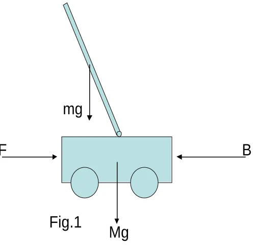
The robot has been modelled as an inverted pendulum on cart system. The principles behind controlling the inverted pendulum on cart system are the same as the principle that govern the control of the two wheel robot. Figure below is a picture of the inverted pendulum on cart system. The picture includes the external forces acting on the system. Where:
· F is the driving force of the motors through the axle of the wheels
· B is the frictional force opposing the motion of the cart-pendulum system
· Mg is the force of gravity on the cart alone
· mg is the force of gravity on the pendulum alone.
F
B
Mg
mg
[image:16.612.214.463.394.639.2]3.11 Free-body Diagram of the Cart
F
R1
R2
Mg
B
P
N
x
Fig.2
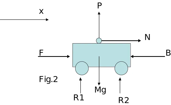
Where;
· P is the vertical force on the cart by the pendulum
· N is the horizontal force on the cart by the pendulum
· R1 and R2 are the reaction forces through the wheels.
From the free body diagram of then cart, we resolve forces in the x-direction, we could resolve forces in the y-direction but they do not give any useful equation towards the derivation of the system equations. Forces in the x-direction give the equation 3.1 below.
x
Ma
B
N
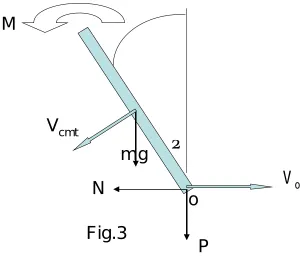
[image:17.612.93.425.137.341.2]3.12 Free-Body Diagram of the Pendulum
o
mg
N
P
V
oV
cmtq
M
Fig.3
Where;
· M is the moment of force about point ‘o’ due to forces N and P
· Forces N and P are the force on the pendulum due to the cart resolved in the x and y directions
· Vcmt is the velocity of the mass center of the pendulum
· Vo is the velocity of point ‘o’ , which is in the x-direction
· q is the displacement angle of the pendulum from the vertical
[image:18.612.132.432.131.392.2](3.2)
From equation 3.2 we derive equation 3.3, which is the velocity of the mass centre relative to the inertial frame or the absolute velocity of the mass centre of the pendulum.
(3.3) To get the absolute acceleration of the mass centre the absolute velocity derived in equation 3.3 above is differentiated. The resulting acceleration is given in equation 3.4 below;
(3.4)
The equation is given in vector notation as the other equations before it.
Now after finding the equation of acceleration of the mass centre of the pendulum, the summation of forces can be done. Summing the forces in the x-direction we get the next equation 3.5. To derive this equation the x-component if the acceleration above is used and the y-component is ignored.
(3.5)
Summing forces in the direction give another equation, equation 3.6. Here the y-component of the acceleration is used and the x-y-component is ignored. Hence equation 3.6 below;
(3.6)
Finally summation of moments about the mass centre gives the last equation, equation 3.7
(3.7)
j i
Vcmo = -lq&cosqr-lq&sinqr
j
i
x
Vcm
=
(
&
-
l
q
&
cos
q
)
r
-
l
q
&
sin
q
r
j
i
x
a
=
(
&&
-
l
q
&&
cos
q
+
l
q
&
2sin
q
)
r
-
(
l
q
&&
sin
q
+
l
q
&
2cos
q
)
r
x
m
ml
ml
N
=
q
&
&
cos
q
-
q
&
2sin
q
-
&
&
mg
ml
ml
P
=
q
&&
sin
q
+
q
&
2cos
q
-q
q
q
Pl
Icm
&
&
Nl
-
=
Substituting equations 3.5 and 3.6 in 3.7 gives equation 3.8 below.
q
q
q
(
)
sin
cos
ml
2I
mgl
x
ml
&
&
-
+
&
&
=
-
(3.8)Substituting equation 3.5 in 3.1 and simplifying by putting like terms together give equation 3.9
q
q
q
q
cos
sin
)
(
M
+
m
x
&&
-
ml
&&
=
F
-
B
x
&
-
ml
&
2 (3.9)The next step is to solve equations 3.8 and 3.9 simultaneously for the second derivative of the tilt angle. The process involves a lot of algebra to simplify the equation. The final product is the equation 3.10 below;
q
q
q
q
q
q
&&
=
ml
/
S
{[
F
-
B
x
&
]
cos
-
ml
&
2cos
sin
+
(
M
+
m
)
g
sin
} (3.10)Where;
·
S
=
ml
2(
M
+
m
sin
2q
)
+
I
(
M
+
m
)
Equations 3.8 and 3.9 are solved simultaneously again for the second derivative of x. The process is quite long and involved like solving for the second derivative if the angle. The outcome is equation 3.11 below;
}
sin
cos
)
(
]
sin
)[
{(
/
1
S
I
ml
2F
B
x
ml
q
2q
ml
2g
q
q
x
&
=
+
-
&
-
&
+
&
(3.11)Equations 3.10 and 3.11 are the equations that model the cart-pendulum system. These equations are not linear. The system is linearized about small deflections of theta, the tilt angle. It is linearized so that the methods of linear systems can be applied to analyze and control the system. Therefore in order to linearize the system theta is restricted to small deflections about the origin, which is the vertical position.
Then: cosq» 1 Sinq»q
q&2sinq »0
The linear equations are as follows;
]
)
(
[
/
q
q
&&
»
ml
S
F
-
B
x
&
+
M
+
m
g
} ]
)[ {(
/
1 S I ml2 F Bx m2l2gq
x&&» + - & +
2 )
(M m mMl
I
S » + +
From the system equations the state space model of the system is derived as below;
Chapter 4
4.1 Estimation theory
To successfully control a system, accurate information about the states of a system at every point in time is required. However to obtain accurate information about a system isn’t an easily achievable task. For starters, the very model that represents the system is not the exact representation of the system; it’s a close approximation of the system behaviour. When modelling a system only the most significant behaviours are modelled and therefore some behaviours which are not deemed important are not modelled. There is a trade off made between capturing most of the system’s behaviour and simplifying the model. Secondly dynamic systems are not only driven by the control inputs, there are also some disturbances which alter the behaviour of the system but are not modelled. These are just two of the many reasons that make correct estimation of the system states a difficult task. To add on to these, sensors that are used to measure the output signals from the system are themselves not accurate and do not provide perfect information. Their signals are corrupted with noise and distortions. Having said all that, it is still imperative to retrieve system information that is as close to the actual information as possible. To obtain accurate data from noise corrupted observations and inaccurate models the estimation theory is used.
Estimation theory is the application of mathematical analysis to the problem of extracting information from observational data (George Siouris). Estimation is characterized as prediction, filtering and smoothing. George Siouris defines prediction, filtering and smoothing as the following:
Prediction means extension in some manner of the domain of validity of the information. Filtering refers to the extraction of the true signal from the observation and smoothing usually refers to the elimination of some noisy or useless components of the data.
dynamic system is to be estimated. Lastly predictors use observations strictly prior to the time that the state of the dynamic system is to be estimated. There are different tools that are used to try and predict the actual states of the system to a high degree of certainty as possible. These include the Wiener filter and the Kalman filter. The Wiener filter was developed by N. Wiener in 1942. The wiener filter estimates the actual states of a system by minimizing the root mean square of the difference between the actual and the desired output. It is most suitable for stationary processes. Applying the wiener filter to time varying processes is very difficult. The Kalman filter is by far t he best linear estimator there is. The Kalman filter estimates the correct states of the system in the presence of disturbances and measurement noise. It even has the ability to estimate the states of a system that cannot be fully modelled or precisely modelled. It can closely predict past, present and even future events
4.2 Kalman filter
The Kalman filter is a linear optimal observer; it uses all the information given to it to compute the best estimation of the state variables. The performance index of this optimal observer is the error covariance. The object is to minimize the error covariance, which is minimizing the mean squared error in the state estimates. The Kalman filter provides the best estimate of the states in the presence of measurement noise and process noise. It works as filter that filters off the noise from the sensors and the process inputs. The kalman filter can be steady-state or changing with time. The time varying kalman filter computes the optimum observer gains each time the filter is updated (Ledin, 2004). The result is an optimal estimate of the state at every step.
4.3 The Discrete Kalman Filter
A kalman filter generally works with a discrete-time time process that is governed by the linear stochastic difference equation;
1 1
1 -
-- + +
= k k k
k Ax Bu w
And a measurement equation;
k k k Hx v
z = + (4.2)
The random variables w and v are the process and measurement noise respectively. These random variables are assumed to have a normal probability distribution with mean zero and covariances Q and R respectively. They are also assumed to be independent of each other or white noise.
The kalman algorithm works in two steps, in the first step the algorithm predicts the state estimates forward in time. That is the algorithm make a prediction of the state estimate of time t, before a measurement at time t is taken. The estimate from this first step is called the ‘a priori’ state estimate. The set of equations used in the first step are called the time update equations. The next step is to get feedback from the sensors and then update the ‘a priori’ state estimates with the feedback from the sensors. The updated state estimate is called the ‘a posteriori’ state estimate. The ‘a posteriori’ state estimate is a linear combination of the ‘a priori’ state estimate and the measurement update from the sensors. The following equation is the equation of the ‘a posteriori state’ estimate. The kalman filter goes through this cycle of predicting the state estimate forward in time and updating the state estimate with the measurement obtained from the sensors. The ongoing cycle of the algorithm is shown below,
A summary of the steps involved in deriving the Kalman filter equations and the gain matrix K that minimizes the error covariance is as follows. Firstly the equations are separated into the time update and the measurement update equations as shown in the figure 4.1 above. The time update or predictor equations are as follows;
(4.3)
(4.4)
Equation 4.3 calculates the state estimate of the state variablexk. The A and B matrices
are the states and the input matrices respectively. Equation 4.4 calculates an estimate of the error covariance matrix. This is the error between the true state variable x, and the estimate of x. The Q in equation 4.4 is the process noise covariance matrix. The next set of equations is the measurement update equations:
(4.5)
(4.6)
(4.7)
4.4 The Kalman Filter and Sensor Fusion
The following section briefly discussed the Kalman filter as it is used for sensor fusion. The section attempt show how the Kaman filter performs sensor fusion in case of redundant sensors. The Kalman filter fuses measurement from sensors according to covariances. The measurement with a high covariance has little effect on the final state estimate. The equation for the kalman optimal observer gain K or L can also be represented in the form of equation 4.8 below.
(4.8)
Where the P matrix is error covariance matrix, C is the measurement matrix and R is the measurement noise covariance matrix. Expanding out the above equation we get equation 4.9 below.
( )
( )
ú ú ú ú ú û ù ê ê ê ê ê ë é · · = -1 1 11 nn T R R C t P tL (4.9)
From this equation it can be seen that the state estimate correction for measurement is weighted by a gain K, which is calculated from equation 4.9. For noisy measurements, this gain will be small and the measurement correction will not have a big impact on ‘a priori’ state estimate. At the extreme, if the measurement is too noisy that the corresponding gain from equation 4.9 approaches zero, the state estimate will approach the ‘a priori’ state estimate.
Chapter 5
5.1 The Robot Hardware
This chapter discusses the robot hardware which includes the robot chassis, the drive system, actuators, sensors and the controller.
5.2 Chassis
5.3 Drive System
The assembly was bought from Oatley Electronics.
5.4 Actuators
5.6 Sensors
The robot uses three sensors which are mainly for balancing the robot. The sensors are the rate gyro, axis accelerometer and inclinometer. The first two sensors are for measuring the tilt rate while the third sensor is for measuring the tilt angle. Two sensors are used for the tilt rate mainly to provide redundancy and hence improved precision. Furthermore the accelerometer provides the static tilt information, when the robot is not accelerating and the gyroscope provides the dynamic tilt information. The gyro also has a drift problem and the accelerometer works to correct that.
5.61 Rate Gyroscope
5.62 Accelerometer
The accelerometer used is an ADXL213 dual axis accelerometer with signal conditioned, duty cycle modulated outputs. The outputs are digital signals whose duty cycles are proportional to acceleration. The duty cycle outputs can be duty measured by a microcontroller without an A/D converter. The sensor operates on 5V DC.
5.63 Inclinometer
The tilt sensor used is an Accustar single axis sensor. This sensor is a capacitance based sensor, when rotated about its sensitive axis the sensor produce a linear variation in capacitance. The capacitance is electronically converted into angular data. The sensitive axis of the sensor is the z-axis, or the axis perpendicular to the sensor. The sensor has a range of ±60°. The sensor operates on 9Vdc and has a ratiometric output. The output is supply dependant. The midscale output, zero degrees, is half the supply voltage while the scale factor is also supply dependant. Clockwise rotations are positive and anticlockwise rotations are negative. Below is a picture of the tilt sensor.
5.7 Microcontroller
Chapter 6
6.1 Classical Control Methods
Classical control theory is the older of the linear control theories. This theory was developed in the early 19th century. The classical control methods are best suited for single input single output system and they include the root locus and the frequency response methods. Even though the root locus is suited for single input single output systems it can be used to great effect to analyse the multiple input multiple output systems. The root locus is one of the methods that have been used in this project to analyse the robot system
6.2 Modern Control Methods
The modern control methods of linear systems design are relatively new compared to the classical control methods. This class of methods include the state space design and the state space design method and the optimal control methods. There are specially suited for system of multiple input and outputs. The state space technique include the pole placement method, this method affords the designer the flexibility of being able to place the close loop poles anywhere that they want. The method is much easier to use than the classical control method. Choosing the best possible locations for the poles is not easy though, especially for higher order systems. The optimum design method is superior to the pole placement and is discussed in the next section.
6.3 Optimum Control
Chapter 7
7.1 Linear Quadratic Regulator
The linear quadratic regulator is the optimum controller that satisfies the following scalar cost function or the performance index.
( )
ò
¥
+ =
0
Rudt u Qx x u
J T T (7.1)
The control method involves finding the closed loop gain matrix K that minimises the performance index. After finding the gain matrix K, the closed loop pole locations are found. The pole locations that results from this method are the best pole locations that could be found. This method involves finding the control law that drives the states of the system as fast as possible at the lowest control force possible. It finds the best compromise between the speed and the control force. This is a very important attribute of the linear quadratic regulator. It ensures that actuator saturation does not happen. It also ensures that the system is not driven too hard and out of the region where the linear approximation of the system holds. For the robot system, too much control force would tilt the robot too far and it wouldn’t be able to return it back to the balanced position.
Chapter 8
8.1 Control System Design
To analyse the system and design a control system matlab and matlab control system toolbox were used. Using matlab and matlab control system toolbox simplified the task of analysing the problem and designing a control system for the problem. This is mainly due to the fact that there are a lot of control systems commands both in matlab and the control system toolbox. Therefore a lot of problems can be solved by using a single command rather than having to write a program to solve the problem. Another reason is that there are a lot of software modules written in matlab available in the internet, which are useful in control systems design. With a bit of luck a relevant software module for the task at hand can be found in the internet and with a little bit of modification the module can be used. In the design and analysis stage two control methods were tried. The first method to be tried was the root locus method.
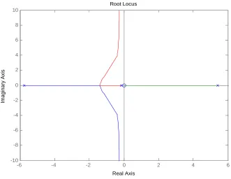
8.2 Root Locus Technique
-6 -4 -2 0 2 4 6 -10
-8 -6 -4 -2 0 2 4 6 8 10
Root Locus
Real Axis
[image:38.612.121.452.92.348.2]Imaginary Axis
Fig 8.1
The system has four poles and two zero. One of the poles is next to -6 and the other is just next to the origin. Another pole is at the origin and the last one is next to 6. The zeros are at the origin. The system is not stable because it has a pole in the right pane of the complex plane.
0 0.5 1 1.5 2 2.5 0
10 20 30 40 50 60 70 80 90 100
Cart Pendulum
Fig 8.2
8.3 Controller Design with the Root locus
To produce the root locus shown in figure 8.1, one pole at the origin cancelled one zero at the origin leaving one zero, the pole out near -6 and the pole near the origin move toward each other and they meet somewhere next to -2. These poles then break away from the real axis and move in opposite directions, asymptotically to the complex axis. The pole on the right side of the complex plane moves towards the zero at the pole origin and terminates there. To pull the branch on the right side of the complex a number of steps are followed. The first step is to add a pole at zero. The pole at zero changes the root locus to the one shown I figure 8.3.
-20 -15 -10 -5 0 5 10
-20 -15 -10 -5 0 5 10 15 20
Root Locus
Real Axis
Imaginary Axis
[image:40.612.119.445.280.545.2]Fig 8.3
The compensator is implemented by adding a zero next to the pole at the origin but to the left of the pole. A pole is added together with this zero and is placed between the zero and the pole out at -6. Next, another zero is added between the recently added pole zero pair and a corresponding pole is also added but it is placed further out in the negative real axis. The result is a lead- lad compensator and the root locus is shown in figure 8.4 below.
-10 -8 -6 -4 -2 0 2 4 6 8 10
-10 -8 -6 -4 -2 0 2 4 6 8 10
Root Locus
Real Axis
[image:41.612.124.476.244.519.2]Imaginary Axis
8.4 Linear Quadratic regulator Design
As already mentioned in the previous chapters, the linear quadratic regulator operates by working out closed loop pole locations that are the best pole locations that satisfy a given performance criterion. The performance criterion for the linear regulator is as follows;
( )
ò
¥
+ =
0
Rudt u Qx x u
J T T (8.1)
The objective is to find a control law that minimizes the performance criteria. To design a linear quadratic regulator in matlab, a matlab control system toolbox command lqr() is used for LQR design in continuous-time. With this command, the work is mainly in the selection of appropriate Q and R weighting matrices. Given the condition that these matrices should be positive semi-definite, it is best to set up these matrices so that only elements along the diagonal are none zero and nonnegative. The best starting point is to initialize both Q and R matrices as identity matrices. Setting up these matrices as identity matrices weighs each input and state variable equally. However, because there is only one input to the system, the R matrix reduces to a constant. After setting up the weighting matrices it is just a matter of calling the lqr() command with the linear plant model and the weighting matrices as the input arguments. The command computes the gain matrix K which is then used to compute the closed loop pole locations. When implementing the regulator, an assumption that all states are available for feedback is made. After the poles have been calculated it is essential to evaluate the performance of the resulting controller.
To evaluate the performance of the resulting controller another matlab function called plot poles was used. This function was written in 2003 by Jim ledin, and it simply plots the new poles of the system together with the performance constraints. Below is a plot of the closed loop poles potted using the plot poles function.
-8 -6 -4 -2 0 2 4
[image:43.612.136.484.140.441.2]-5 -4 -3 -2 -1 0 1 2 3 4
Fig 8.5
than the other to get the system to stabilize. For example the wheels should move in the direction that the robot is falling faster than the rate at which the robot is falling so as to keep the robot balance. Therefore the robot’s horizontal speed was given a higher weight than the robots tilt rate.
-4 -3.5 -3 -2.5 -2 -1.5 -1 -0.5 0 0.5 1 -2
-1.5 -1 -0.5 0 0.5 1 1.5
Fig 8.6
As can be seen from the plot the two closed loop poles nearer to the origin no longer fall within the specified constraints. Therefore the desired system response was obtained after a number of iterations to get a correct compromise between the response speed of the states and the control effort. This is a very desirable property of the linear regulator control design which helps to avoid saturation of the actuator or clipping of the control effort
8.6 Optimal Observer Designer
[image:45.612.125.472.105.374.2]the kalman filter works as both a filter and an estimator. It does not only estimate those states that are not measured or that we don’t have sensors for but it also estimates the true states of the measured variables. This is because even though thee variables are measured, there are sensor measurements are corrupted by noise and inaccuracies in the model of the system. To create the kalman filter, a matlab control toolbox command called kalman() is used. To use the kalman command the plant model has to be represented as linear stochastic model rather than the deterministic model. The stochastic model includes the process noise model and the measurement noise model together with their respective covariance matrices. Given the plant stochastic model as its input argument, the command computes the optimal observer gain matrix L.
8.61 Linear Stochastic Model
The plant linear stochastic model is shown below;
v
Hw
Du
Cx
y
Gw
Bu
Ax
x
+
+
+
=
+
+
=
&
being the process noise and the R being the measurement noise. The Q matrix is an r x r matrix, where r is the number of plant inputs. The diagonal elements of Q represent the corresponding noise variance on each input. The matrix can be initialized as an identity matrix and the diagonal elements adjusted to get a satisfactory observer performance. For the robot system, the Q matrix is a constant since there is only one input to the plant. The measurement covariance matrix R is also a diagonal matrix, with each element along the diagonal containing the variance of the error in the corresponding sensor measurement. The error can be determined from the manufacturer-provided data describing the sensor error characteristics. The error variance is computed by squaring the root mean square jitter error specification from the sensor manufacturer’s data sheet. The units of each diagonal must be the square of the units of the corresponding plant output.
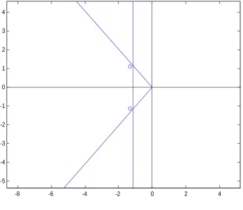
The next stage in the design process is to implement the combined observer-controller for the plant. Below is a plot of the observer-controller poles of the system.
-180 -160 -140 -120 -100 -80 -60 -40 -20 0 -60
-40 -20 0 20 40 60
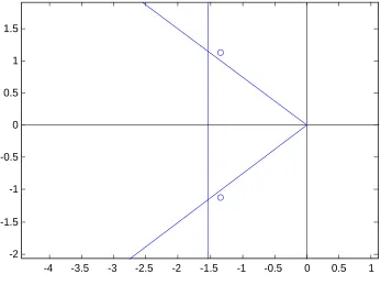
[image:47.612.125.455.411.658.2]The left most poles in the diagram are the closed loop poles of the system and the next set of poles form the left are the observer poles. The other set of observer poles are near the origin but further right than the closed loop poles next to them. Below is a close view of the set of poles near the origin.
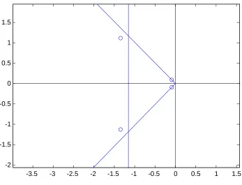
-3.5 -3 -2.5 -2 -1.5 -1 -0.5 0 0.5 1 1.5 -2
[image:48.612.126.473.204.469.2]-1.5 -1 -0.5 0 0.5 1 1.5
Fig 8.8
0 0.5 1 1.5 2 2.5 3 3.5 4 4.5 -0.3 -0.25 -0.2 -0.15 -0.1 -0.05 0 0.05 0.1
From: r (m)
To: theta (
rad
)
Step Response
Time (sec)
Amplitude
0 0.5 1 1.5 2 2.5 3 3.5 4 4.5
-0.3 -0.25 -0.2 -0.15 -0.1 -0.05 0 0.05 0.1
From: r (m)
To: theta (
[image:49.612.114.486.84.352.2]rad ) Step Response Time (sec) Amplitude Fig 8.9
8.7 Feed-Forward Gain
gain is selected to scale the reference inputs to produce steady-state error at the outputs. The following equation is used to compute the gain N;
x u KN N
N = + (8.2)
The K is the controller gain calculated from the regulator design method and the matrices Nu and Nx are determined form the plant model as shown below;
ú û ù ê ë é ú û ù ê ë é = ú û ù ê ë é -I D C B A N N u x 0 1 (8.3)
0 0.5 1 1.5 2 2.5 3 3.5 4 4.5 -0.2 0 0.2 0.4 0.6 0.8 1 1.2
From: r (m)
To: x(m ) Step Response Time (sec) Amplitude
0 0.5 1 1.5 2 2.5 3 3.5 4 4.5 -0.2 0 0.2 0.4 0.6 0.8 1 1.2
From: r (m)
[image:51.612.106.485.81.340.2]To: x(m ) Step Response Time (sec) Amplitude Fig 8.10
The optimum controller and observer have designed in the continuous-time domain. However the controller of the robot is going to be ran in a microcontroller which means the controller has to operate in discrete-time domain. Therefore the controller has to be transformed into the discrete-time domain. It is possible to change o the discrete time domain right at the start of the design process and then working in that domain all through to the finish. This however could present some problems in the design process. The problem could rise when a wrong sampling period is chosen for the implementation of the discrete controller. The thing is that all the computations that are made in the design process are dependant on the chosen sampling period and if it turns out that the sampling period chosen is not the right one then all the computations would have to be repeated for the correct sampling period. This obviously would be a tedious process. Therefore transforming the controller to the discrete-time domain saves a lot of design time.
system closely follows the continuous system but the microcontroller would have to do a lot of computations. This would require a more powerful micro controller with a bigger memory. Naturally, this means a more expensive processor. On the other extreme, when the sampling period is too big the discrete time controller’s performance would diverge from the continuous time controller performance. When the sampling period is too big it can even lead to excessive overshoot, oscillation or even instability of the closed loop system.
8.9 Choosing A Sampling Period
.From the preceding discussion it is obvious that choosing of a sampling period is very critical for the success of the controller. A very important condition for the selection of a sampling period is the nyquist sampling theorem. By the sampling theorem, the sampling frequency must be at least twice the highest significant frequency in the controller input signal to enable processing by the controller. To help in the selection of a suitable sampling period a methodical approach to the problem has been adopted. The method was adopted from the book called embedded control systems in c/c++ by Jim Ledin. In the book, Jim proposes the following steps;
1. Plot the step response and the frequency response If the closed- loop system. 2. Choose a very short sampling period that provides a good discrete-time system
approximation to the continuous-time system performance.
3. Discretize the control system with the c2d() command and appropriate discretization method.
4. Plot the step response and the frequency response of the closed-loop system using the discretized controller in place of the continuous-time controller. 5. Increase the sampling period and repeat steps 3 and 4. Continue until the step
The above steps give an idea of how big a sampling period the system can tolerate. However a more conservatively smaller sampling period is chosen to accommodate the nonlinearities in the system. The results of using the above method are given below. However I used the open- loop system responses instead of the closed- loop system responses. This is because my closed- loop responses did not give a clear picture that would help me to arrive at meaningful conclusions. The figure below shows the open-loop continuous and discrete-time responses for a sampling period of 0.1 milliseconds.
0 0.01 0.02 0.03 0.04 0.05 0.06 0.07 0.08 0.09 0.1 0
0.05
Time, seconds
Response
continuous foh
10-3 10-2 10-1 100 101 102 103 -200
-100 0
Magnitude, dB
10-3 10-2 10-1 100 101 102 103 -100
-50 0
Frequency, rad/sec
Phase, degrees
[image:53.612.107.480.258.544.2]Fig 8.11
The discrete-system closely follows the continuous response and there is no divergence what so ever for the given frequency range.
discrete-time system accurately follows the continuous- discrete-time system for the given frequency range.
0 0.01 0.02 0.03 0.04 0.05 0.06 0.07 0.08 0.09 0.1 0
0.05
Time, seconds
Response
continuous foh
10-3 10-2 10-1 100 101 102 103 -200
-100 0
Magnitude, dB
10-3 10-2 10-1 100 101 102 103 -100
-50 0
Frequency, rad/sec
Phase, degrees
[image:54.612.105.479.150.435.2]Fig 8.12
0 0.01 0.02 0.03 0.04 0.05 0.06 0.07 0.08 0.09 0.1 0
0.05
Time, seconds
Response
continuous foh
10-3 10-2 10-1 100 101 102 103 -200
-100 0
Magnitude, dB
10-3 10-2 10-1 100 101 102 103 -100
0 100
Frequency, rad/sec
Phase, degrees
[image:55.612.106.477.91.380.2]Fig 8.13
Chapter 9
9.1 Discretization Method
The last consideration in implementing a discrete-time controller is the discretization method used. There are a number of discretization methods available, each with its own advantages and disadvantages. The disretization methods available in matlab are the zero-order hold method, first-order hold method, the pulse-invariant discretization method, the bilinear approximation method, the bilinear approximation with frequency prewarping and lastly the matched pole zero method. The matched pole- zero method is only applicable for SISO systems as a result it us not considered for this problem. The following is a brief description of each method and their suitability.
From the above discussion the best two methods are the zero-order hold and the first-order hold methods because they are general purpose methods and do not need any special condition. Between the two methods the first-order hold method is superior and it is therefore the chosen method for the discretization process.
Chapter 10
10.1 Motor control
This section discusses pulse width modulation control of the motor and it also touches on the use of an H-Bridge amplifier for the bidirectional control of the motor.
10.2 Pulse Width Modulation.
microcontroller does not have it. Another benefit of using the PWM is that the signal remains digital and no digital-to-analogue conversion is necessary, by doing so the noise effects are minimized.
10.3 The H-Bridge Amplifier
Chapter 11
11.1 Hardware Configuration
To set up the hardware of the system for correct software control, the hardware needs to be configured. The two most important peripheral devices used in the system ore the analogue-to-digital converter and the pulse-width modulator.
The analogue to digital converter is used to interface the sensors of the system to the microcontroller. There are four sensors used for the robot system. All the sensors produce an analogue output proportional to the state measurement they are measuring. The analogue signals from the sensors need to be converted to digital signals for microprocessor processing. As a result the analogue-to-digital converter is used to interface the sensors and the microprocessor for this reason. For correct operation, the analogue-to-digital converter needs to be configured. The microprocessor has eight ADT channels and the four sensors are connected at channels 0 to 4. The ADT unit has a control register 2 associated to each channel. The most important bits in these registers are the AFFC, the DJM, the ASCIE and the ASCIF. The ASCIE is the Sequence Complete Interrupt Flag, this bit is set to enable an interrupt function to signal the MCU when the conversion is complete. This way the MCU can proceed with other operations and not have to keep checking the ADT to see whether a conversion is complete. The ASCIF is the Sequence Complete Interrupt Flag, this bit is set to enable the flag to be set when a conversion complete interrupt happens. This bit is cleared when the conversion complete interrupt is serviced. Last but not least the AFFC is the Fast Conversion Complete Flag Clear. This bit is set to enable the Sequence Complete Interrupt Flag to be automatically cleared by reading the conversion results from the data port. And finally the DJM is the Register data justification mode. The bit is set for either left justification or right justification of the data in the data register.
data registers according to the sequence at which the conversions occur. The result of the first conversion appears in the first result register and so on. Bit 3 of the register, which is S1C controls the conversion sequence length together with bit 6 of control register 5. For the operation of the robot system these bit have been configured four conversions per sequence. In the control register 4, the resolution of the ADC has been set to 10 bit resolution by setting bit 7. The ADC clock is set to a quarter of the system clock by setting appropriates bits in register 4. The sample time is set to 2 A/D clock periods. The ADC is set for continuous conversion mode setting SCAN bit in control register 5. Lastly the MULT bit in control register 5 is set to allow the ADC sequence control to sample across many in a single sequence. Bits CC, CB and CA are all cleared to start sampling from channel 0.
Chapter 12
12.1 Encountered Difficulties
Chapter 13
13.1 Foreseeable Problems with my Robot System.
Chapter 14
14.1 Risk Analysis
There are risks involved in the construction of the robot and its use. The first and maybe the biggest risk is in the building of the robot chassis. The chassis is constructed from steel plates. To machine these steel plates powerful machine with sharp cutting tools are used. These machines need skilled personnel to operate and they also need a lot of care. If not care is not taken when operating these machines, serious injuries may result such as loss of limbs. Another risk associated with robot construction is in dealing with a high voltage sources. The motors are operated from 24 V sources and even the lesser 12V sources are used, the risk is still high. The risk of damaging the electrical components, such as the H -Bridge and even the microprocessor itself is even higher. The FET- transistors used in the H-Bridge are particularly sensitive and easy to burn. Some of the electrical components used in the robot are very expensive, and the high cost makes the risk even higher.
During the operating stage of the robot, care needs to be taken as well. The complete robot and the battery weigh just below 10 kg and the body is made of sharp steel plates. The harm that this robot can cause on the people operating the robot if it accidentally falls on them could be great especially that the robot is heavy and the motors would have to use more power to stabilize the system. The robot could also damage the floor if it falls to the ground.
Chapter 15
15.1 Costs of Producing the Robot
The costs involve in the building of the robot are quite substantial. The greater costs are the costs of the Motorola MC68HC912D60A processor. The card12 costs around US$159. The other big cost was in acquiring the tilt sensor. The tilt sensor cost about A$150. These are the two big costs, apart from that the drive system costs around A$100 and the battery was A$24. Other costs include the costs of building the body of the robot chassis, which include the labour costs of machining.
Chapter 16
References
Clark, R.N. 1996, Control System Dynamics, Cambridge University Press.
Dorf, R. C. 1989, Modern Control Systems, 5th edn, Addison-Wesley Publishing Company.
Nise, N.S, 2004, Control Systems Engineering, 4th edn, John Wiley & Sons
Stefani, S.T. et al, 1994, Design of Feedback Control Systems, 3rd edn, Sauinders College Publishers
http://www.tedlarson.com/robots/balancingbot.htm
http://www.engin.umich.edu/group/ctm/examples/pend/invpen.html.
http://www.geology.smu.edu/~dpa-www/robo
/nbot/
Shinners S. M, 1998, Advanced modern control system theory and design, John Wiley and Sons
Ledin J, 2004, Embedded Control System in C/C++: An Introduction for Software Developers using Matlab, CMP Books
Zhou and Kemin, 1996, Robust and optimal control, Prentice Hall
Westphal L.C, 1995, Sourcebook of control systems engineering, 1st edition, chapman & Hall
Greenside L. A, 1970, Elements of Modern Control Theory, Mcmillian & Co
Siouris G.M, 1996, Optimal Control and estimation Theory; John Wiley and Sons
Friedland B, 1996, Advance Control System Design, Prentice Hall
Mohinder S & Andrews A, Kalman filtering: Theory and Practice using Matlab, 2nd, A Wiley-Interscience Publication
Welch G & Bishop G, 2006, An Introduction to the Kalman Filter
Bak T, 2006, Estimation and sensor Fusion.
Maybeck P.S, 1979, ‘Stochastic models, estimation, and control’, Academic Press
APPENDIX A: PROJECT SPECIFICATION
University of Southern Queensland
FACULTY OF ENGINEERING AND SURVEYING
ENG 4111/4112 Research Project
FOR: Kealeboga Mokonopi
TOPIC Balancing a two wheeled robot
SUPERVISOR: Mr Mark Phythian
SPONSORSHIP: Faculty of Engineering and Surveying, USQ
PROJECT AIM: The aim of this project is to design and building a two wheeled robot system,
PROGRAMME:
1. Literature Review
2. Producing a mathematical model of the system. 3. Suitable control system investigation
4. Control system implementation 5. Hardware design.
As time permits:
1. Control the robot to a predetermined position 2. Make the robot system to turn
AGREED
________________ (Student), _______________(Supervisor)
APPENDIX B MATLAB CODES
============================================================
% The code is used to determined the controllability of the system %Produced by Kealeboga Mokonopi
%University of Southern Queens land % 2006
%====================================================================
function controllabilitymatrix
% System Variables
M = 0.5; m = 0.2; b = 0.1; i = 0.006; g = 9.8; l = 0.3;
p = i*(M+m)+M*m*l^2;
% Production of system amtrices
A = [0 1 0 0; 0 -(i+m*l^2)*b/p (m^2*g*l^2)/p 0; 0 0 0 1; 0 -(m*l*b)/p m*g*l*(M+m)/p 0]; B = [0; (i+m*l^2)/p; 0; m*l/p];
Cm = ctrb(A,B) Rank = rank(Cm)
============================================================================================================== ============================================================================================================
% The code is used to determined the observability of the system %Produced by Kealeboga Mokonopi
%University of Southern Queens land % 2006
%====================================================================
function observabilitymatrix
%system variables and system amtrices
M = 0.5; m = 0.2; b = 0.1; i = 0.006; g = 9.8; l = 0.3;
p = i*(M+m)+M*m*l^2; %denominator
A = [0 1 0 0; 0 -(i+m*l^2)*b/p (m^2*g*l^2)/p 0; 0 0 0 1; 0 -(m*l*b)/p m*g*l*(M+m)/p 0]; B = [0; (i+m*l^2)/p; 0; m*l/p];
===================================================================== % The function implements the continous time controller
% using the linear regulator and kalman observer % Produced by Kealeboga Mokonpi
% USQ, 2006
function lqrcontrl
%==================================================================== % system variables and constants and system matrices
M = .5; m = 7; b = 0.1; i = 0.523; g = 9.8; l = 0.25;
p = i*(M+m)+M*m*l^2;
A = [0 1 0 0; 0 -(i+m*l^2)*b/p (m^2*g*l^2)/p 0; 0 0 0 1; 0 -(m*l*b)/p m*g*l*(M+m)/p 0]; B = [ 0;
(i+m*l^2)/p; 0; m*l/p]; C = eye(4); D = [0];
ssplant = ss(A,B,C,D);
%======================================================================
set(ssplant, 'InputName', 'Cart Force');
set(ssplant, 'OutputName', {'Cart Pos', 'Cart Vel', 'Pend Angle', 'Pend Vel'});
set(ssplant, 'StateName', {'Cart Pos', 'Cart Vel', 'Pend Angle', 'Pend Vel'});
% Design the controller gain
Q = diag([1e9 1e6 1e10 1e5]); R = 1;
K = lqr(ssplant,Q,R);
%Compute the feedforward gain
Cn=[1 0 0 0];
N=feedforwardG(A,B,Cn,0,K)
cl_sys = feedback(ssplant, -K,+1)
% t_settle = 3; % damp_ratio = 0.8;
% % Design the observer gain
a = ssplant.a; b = ssplant.b;
c = [1 0 0 0; 0 0 1 0; 0 0 0 1]; d = [0; 0; 0];
QN = 0.1^2;
g = b; h = d;
obs_plant = ss(a, [b g], c, [d h])
[kest, L] = kalman(obs_plant, QN, RN)
% Create a state space observer-controller
ssobsctrl = ss(a-L*c, [L b-L*d], -K, 0)
% % Augment the plant model to pass the inputs as additional outputs
r = size(b, 2); % Number of inputs
n = size(a, 1); % Number of states
ssplant_aug = ss(a, b, [c; zeros(r, n)], [d; eye(r)]);
% Compute the feedforward gain
Cn=[1 0 0 0];
N=feedforwardG(A,B,Cn,0,K)
% Form the closed loop system with positive feedback
sscl = N*feedback(ssplant_aug, cl_sys, +1); figure
plotpole(sscl, t_settle, damp_ratio);
%Plot the step response
set(sscl,'InputName','r (m)', 'OutputName', {'x(m)', 'theta (rad)',
'angularrate(rad/s)', 'F (N)'}); figure
function plot_poles(sscl, t_settle, damp_ratio)
=======================================================================
%PLOT_POLES Plot system pole locations with settling time and damping ratio constraints.
%
% PLOT_POLES(SSCL, T_SETTLE, DAMP_RATIO) %
% This function plots the pole locations for the closed loop % system SSCL along with the settling time constraint
% T_SETTLE (in seconds) and damping ratio DAMP_RATIO.
% By Jim Ledin, 2002.
=======================================================================
plot(pole(sscl), 'o')
axis equal
a = axis;
x_min = a(1); x_max = a(2); y_min = a(3); y_max = a(4);
settling_pct = 0.01; % If no settling percentage given, use 1%
settling_limit = -log(settling_pct) / t_settle;
if x_max < -settling_limit + 0.1*(x_max - x_min) x_max = -settling_limit + 0.1*(x_max - x_min); a(2) = x_max;
end
hold on
plot([x_min x_max], [0 0], '--k') plot([0 0], [y_min y_max], '--k')
plot([-settling_limit -settling_limit], [y_min y_max]);
angle = acos(damp_ratio);
plot([x_min 0 x_min], [x_min*tan(angle) 0 -x_min*tan(angle)])