OptiFlow - a capacity management tool

OptiFlow - A Capacity Management Tool

Robert Suryasaputra

, Alexander A. Kist

and Richard J. Harris

School of Electrical and Computer Engineering

RMIT University Melbourne, GPO Box 2476V, VIC 3001, Australia Email: rsuryasaputra@gmail.com, kist@ieee.org

†_{Institute of Information Sciences and Technology}

Massey University, Private Bag 11 222, Palmerston North, New Zealand Email: R.Harris@massey.ac.nz

‡_{Corresponding author}

Abstract— Intra-domain traffic engineering for routing proto-cols such as OSPF (Open Shortest Path First) or Intermediate System-Intermediate System (IS-IS) can be performed by finding a judicious set of weights to allocate to the links of the network. Unfortunately, methods proposed in the literature for finding those weights may require a significant computational effort. By way of contrast, weight setting approaches based on Linear Programming can be shown in this paper to find suitable weights in the order of seconds. Prior to this time, it was necessary to determine appropriate weight settings in an off-line mode. From the results presented in this paper it can be demonstrated that solutions can be located for this problem in a matter of seconds. This makes it possible to perform traffic engineering for short term link overloads in real-time mode. The performance of this methodology has been verified by using simulation based on the well-known performance tool, ns-2. The technique described in this paper is being integrated into an optimisation module of a network capacity management tool called OptiFlow.

I. INTRODUCTION

Recent years have seen a tremendous growth in Internet traffic. This on-going development increases the need of Internet Service Providers (ISPs) to operate and manage their networks effectively to avoid congestion for their customers’ traffic flows. However, native IP networks have limited traffic management capabilities. This is particularly true for Open Shortest Path (OSPF) type networks. Unfortunately, ISPs only have a limited number of software systems and tools to support the management aides in measurement and control activities [1]. As a result, network managers and operators have limited knowledge of network dynamics from a global perspective. (There are many measurement and monitoring systems for

individual links or routers, but few systems permit a more

holistic view.)

Link congestions can occur in these networks and is usually caused by network component failures, scheduled mainte-nance, traffic shifts or mis-configurations. In these changing environments, the connectivity is maintained by routing pro-tocols. Intra-domain routing protocols such as Open Shortest Path First (OSPF) [2] or Intermediate System-Intermediate System (IS-IS) [3] compute routing table in set time intervals. The protocols compute the shortest path to all destinations based on link metrics and update the router’s forwarding tables. Although this restores the connectivity, there is no

guarantee that a service quality is maintained. Some links might be congested because they have to carry additional traffic from the failed links.

Congestion can be divided into two categories: Congestion due to uneven traffic distribution and uniform and persistent congestion. The former can be addressed by Traffic Engineer-ing (TE), the later requires capacity expansion or admission control. TE can be applied if traffic is not mapped efficiently to the available network resources, i.e. there are network parts that have to sustain more than the allowable load despite there is ample network capacity. These congested areas are usually referred to as “hot spots”. Generally, ISP networks are well dimensioned and have sufficient capacity. For example, Sprint, one of the largest (tier-1) ISPs in the USA, over-provision their network by maintaining the maximum utilisation of any links to be below 50%. The average link utilisation is between 20 - 25% [4] [5]. In situations where capacity is available, traffic engineering is an efficient alternative to capacity expansion.

In [6] it is shown that intra-domain traffic engineering can be performed by changing link metrics/weights (both terms are interchangeable and carry the same meaning). The aim of this work was to change a few weights to remove hot spots instead of changing many weights what could be disruptive to network traffic. Disadvantages of this method include the exhaustive calculations that are required to determine new weight sets. Experiments done on 100 node network took about 1.5 hours; a less exhaustive search reduced this to 15 minutes, with an optimality trade-off [7].

Previous work by Murphy et al. [8] proposed a fast weight setting approach based on Linear Programming (LP). For the similar network size as mentioned above, a few weight changes can be obtained in less than a minute. This set of weights is not necessarily optimal, but the results are much better than the original set. Weight changes can briefly disturb the network, but this outweighs the disturbance that is caused by long-term overloads. For congestion that lasts for less than a minute or two, weight changes are not suitable; they introduce more disturbances in the network.

been implemented and integrated in OptiFlow. Its aim is to combat link overloads and hot spots. This is achieved without changes to current routing protocols and router hardware. Users can also build their own topology, set appropriate configuration and use OptiFlow as a platform to investigate what-if scenarios, e.g. investigating the effect of pre-planned maintenance on the maximum link utilisation.

Secondly, this paper introduces simulation results that demonstrate the performance of the optimisation and validate the LP based weight setting method. The tests use the popular network simulator ns-2 simulator [9].

The paper is structured as follows: Section 2 describes the OptiFlow system architecture and briefly describes its implementation. Section 3 shows the LP problem formulation for the optimisation. Section 4 discusses experiment setup, the simulation results from ns-2 simulator and calculation results for a larger network. Finally section 5 concludes the paper.

II. SYSTEMARCHITECTURE ANDIMPLEMENTATION

OptiFlow is implemented as a Microsoft Windows appli-cation. It is written in C++ and uses ObjectiveStudio for the drawing library [10] and WinSNMPv1 [11] for the SNMP communication. It runs separately on a computer with a direct access to the managed network.

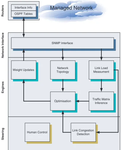
Figure 1 depicts the functional block diagram of OptiFlow. These blocks can be classified into three main groups, namely Network Interface, Engines and Steering. The first group handles the communication between OptiFlow and managed devices, i.e. routers. The second group is the main part of OptiFlow. The modules in this group provide inputs for the optimisation module and translate the output of the optimi-sation module back to the network. The third group is the steering module, which handles user interaction.

SNMP (Simple Network Management Protocol) is an ap-plication protocol that manages the communication between network devices. It is the de-facto standard in network man-agement. In OptiFlow, SNMP is used to obtain OSPF connec-tivity information from a router by reading its Management Information Base (MIB) table. This is then used recursively to discover the network topology. SNMP is also used to obtain information regarding the network interfaces to calculate the link load. It is also used to enable the altering the OSPF metrics.

The live information from SNMP is translated by the network topology module into an internal representation of the network as a directed graph for visualisation of optimisation and measurement data. The link load measurement module periodically calls SNMP function to obtain the number of in-coming or outgoing bytes from a particular interface. Together with the topology information, the link load measurement re-sults are processed by traffic matrix inference module to obtain the OD-Pair (Origin-Destination Pair) traffic matrix, which is required by the optimisation module and the associated man-agement functions. Inference techniques are used to obtain the OD-Pair traffic matrix because direct measurement techniques require greater investments and processing power. The traffic

SNMP Interface

Managed Network

Optimisation Traffic Matrix Inference Link Load Measument Network

Topology

Link Congestion Detection Weight Updates

Interface Info

Human Control

N

etw

ork Interface

E

ngines

S

tearing

OSPF Tables

R

ou

ters

Fig. 1. OptiFlow System Diagram

demand matrix inference problem is known to be a particularly hard problem since it is often highly under-constrained. There are several published works that that propose methods for overcoming this problem, e.g. [12] [13] [14] [15]. OptiFlow implements the inference method known as Tomogravity and it is described in [15].

The optimisation module takes information provided by the network topology and traffic matrix inference modules. The LP optimisation technique used by the optimisation module is described in Section III. The optimisation module builds the LP problem and uses a solution from an LP solver to obtain a set of weight changes. Weight update module then calls appropriate SNMP functions to setup the new link weights in the network.

The GUI Interface module presents the live network infor-mation visually to the user through a ‘canvas’ (see Figure 2). Users can also view or modify the specific properties of the network components, such as link metric. Users can change the link metric manually and commit the changes to the network via SNMP. The interface also allows to trigger the optimisation whenever the user believes that the optimisation is necessary. OptiFlow also has a congestion detection module that triggers the optimisation automatically if one or some link utilisations exceed the preset threshold for a period of time.

The choice of LP solver that is used by the optimisation module is made flexible. Users can choose to use commercial LP solver such as CPLEX [16] or publicly available solver from GNU i.e. glpk [17].

Fig. 2. OptiFlow Functionality

point onwards, users can use OptiFlow as a what-if scenario tool, e.g. investigating an effect of link failures or preplanned maintenance by deleting the network components. OptiFlow then can predict the new set of link utilisations due to those events, and may suggest appropriate weight changes whenever congestion exists. It is possible to use OptiFlow to predict the resulting link utilisation after weight changes are invoked. Hence, users have an informed decision whether the weight changes should be invoked or not.

III. OPTIMISATIONOVERVIEW

This section introduces the theoretical background that underpins the optimisation module in OptiFlow.

A. LP Problem Formulation

Murphy et al [8] have formulated the IP routing problem as a standard multi-commodity flow problem. Suppose that there areKtraffic demands and that there aremunidirectional links. For each commodity k, Pk denotes a collection of directed paths (chains) from the origin node to the destination node, f(P) is the flow on such a path P, c(P) is the cost of the path P andδij(P)is equal to one if link (i, j) is contained in the path P and is zero otherwise. Note that

c(P) =

(i,j)∈P

cij

where cij is the per unit cost of flow on link(i, j). Thus, it

is possible to use the standard path-flow formulation for this model as described in [18]. This greatly reduces the number of constraints but increases the number of path-flow variables. Most of these paths carry zero flow in the optimal solution. This results in the following path-flow formulation of the LP problem:

Minimise

1≤k≤K

P∈Pk

c(P)f(P) (1)

subject to

1≤k≤K

P∈Pk

δij(P)f(P)≤uij (2)

for all links(i, j)whereuij is the capacity of link(i, j)and

P∈Pk

f(P) =dk (3)

where dk is the size of the flow for each commodity for all k= 1, . . . , K and allf(P)≥0.

The advantage of using a path-flow formulation is the huge reduction in the number of problem constraints. The number of constraints in the link-flow formulation is proportional to O(n3), while in the path-flow formulation it is proportional to O(n2). The savings in the number of constraints does come at a cost, because the number of path variables can be enormous. However, it is possible to “limit” the number of path variables as discussed below.

Let Pk contain a list of the paths for OD-Pair k ranked in order of their path costs. The size n of the set of paths, Pk, was actually limited to 10, because few, if any, cases were ever found where flows used greater than seven or eight paths. The list of paths was found via a well-knownk−shortest paths algorithm due to Yen [19]. This was further tested in the optimisation process when it was found that if n = 3 the throughput was significantly reduced but after n = 10, there was no observable difference in overall throughput. The constraints in (3) state that the total amount of flow that is carried on each of the paths associated with an OD-Pair must be equal to the total OD-Pair traffic demand. The constraints in (2) are known as the “bundle” constraints as they tie together all the flows by restricting the amount of flow on a particular link(i, j).

B. The Complementary Slackness Conditions and Shortest Path Routing

The complementary slackness conditions have very inter-esting consequences for the routing problem. The path flow formulation contains a dual variable ωij for each link and

another dual variable σk for each commodity k = 1, . . . , K. Define the reduced cost for pathP,cσ,ω_P , as

cσ,ω_P =c(P) +

(i,j)∈P

ωij−σk

The path flow complementary slackness conditions as stated in Ahuja et al [18] are valid at optimality, viz:

ωij[

1≤k≤K

P∈Pk

δij(P)f(P)−uij] = 0for all links(i, j)

(4) cσ,ω_P ≥0 for allk= 1, . . . , K and allP∈Pk (5)

cσ,ω_P f(P) = 0for allk= 1, . . . , K and allP ∈Pk (6)

It is further stated in [18] that equations (5) and (6) imply that: σk is the shortest path distance from the source node

to the destination node (commodity k) with respect to the

modified costs (cij+ωij) and in the optimal solution every

Routers make their routing decisions independently, based on shortest path computations, which are, in turn, based on a set of link weights for the whole network. From the results above it can be seen that if the modified costs, cij +ωij,

are used as the OSPF weights, then a traffic demand is automatically be routed on a path of cost σk. For demands where only one shortest path of cost σk exists, the actual routing solution is identical to the primal LP solution. Setting the OSPF weights to the modified costs will also initiate cases in which some commodities have multiple paths with equal costσk. In this particular case, the LP primal solution allocates the flow to the paths in an arbitrary manner to these paths. Our method ignores these arbitrary splits and instead makes use of the Equal Cost Multi Paths (ECMP) capability that forms part of the operation of OSPF that is readily available in modern routers employing this routing protocol.

As a consequence of the LP formulation it is noted that for this method, the first few weight changes give the best reduc-tion in the maximum utilisareduc-tion. The LP solureduc-tion procedure removes the most infeasible variables during the dual simplex operation to recover feasibility. The infeasible variables in the problem are congested links.

IV. RESULTS ANDDISCUSSION

This section introduces the experimental setup, the sim-ulation results and the calcsim-ulation results. The objective of running simulations is to observe the improvement generated by the LP based weight setting approach against the default OSPF metric values. The parameter of interest is the number of packets loss.

A. Experimental Setup

The simulated network consists of 8 routers which are connected by 24 uni-directional links as shown in Figure 3. Attached to each of these routers is a workstation that originates and terminates traffic. It is assumed that a work-station generates traffic to each of the other workwork-stations in the network, i.e. there are 56 OD-Pairs in total. The origin is modelled as a constant bit rate source sending 500-byte packets to the destination node. The inter-arrival rate is governed by the size of the OD-Pair demand. There are two types of link capacity, viz: 100 Mbps and 10 Mbps. The link latency is chosen to be 5 ms. The default OSPF metric values for 100 Mbps and 10 Mbps links are 1 and 10, respectively. The simulation length is 20 seconds including a 1 second warm-up period. The collection of statistics starts after the warm-up period has elapsed. The simulation is carried out using the well-known ns-2 simulator [9].

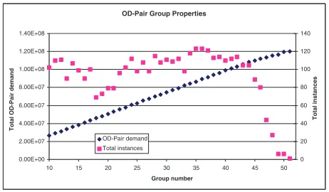
The simulation is done with a number of different traffic matrix instances. There were 3887 instances in this study. These instances were grouped into 42 groups, numbered from group 10 to group 51, according to their total load (see Figure 6 to see how the average load varies among the different groups and how many traffic instances are in a particular group). The statistics are collected for individual instances and then averaged together with the ones belonging to the

Fig. 3. Topology for ns-2 simulation

Avg OD loss

0% 2% 4% 6% 8% 10% 12% 14%

10 15 20 25 30 35 40 45 50

Group

A

v

g

L

o

s

s

(%

)

OSPF OptiFlow

Fig. 4. Average OD pair loss across different groups

Max OD loss

0% 10% 20% 30% 40% 50% 60%

10 15 20 25 30 35 40 45 50

Group

M

a

x

L

o

s

s

(%

)

OSPF OptiFlow

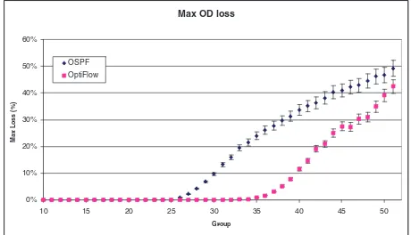
Fig. 5. Maximum OD pair loss across different groups

same group. OptiFlow is used to obtain a weight set for each individual traffic matrix instance. The same simulation set is then run with a weight set obtained from OptiFlow.

B. Simulation Results

across the 56 OD-Pairs. These figures are then averaged to form the group statistics.

With an increasing load, it is expected that the network will start to eventually experience congestion, which results in a number of packets being dropped. The 95% confidence intervals are given as error bars in the results. The simulation shows that with the default OSPF metric the network starts to exhibit packet loss at group 26, whereas the OptiFlow weight set pushes this to group 36 (see Figure 4). At group 35, the standard OSPF protocol gives 5.5% loss but at this point there is still no loss with OptiFlow. With the highest load (group 51), the OptiFlow weight set gives about a 25% relative improvement against the OSPF weight set. OptiFlow weight setting performs better against the default OSPF weight setting across all the groups. However, as might be expected, the advantage gradually diminishes (i.e. the two curves come closer together) as the load increases further. At this point, the network is approaching its saturation point, where there is not much room left to reroute the traffic. When there is no more room to reroute the traffic, no traffic engineering method that involves rerouting would work. Such cases represent general network overloads and as such an alternative mechanism for reducing congestion would be to throttle traffic back at the source via some form of flow control or “call-gapping” equivalent procedure.

Figure 5 depicts the maximum OD-Pair loss across the different groups. As it is the case with the average packet loss, the OptiFlow weight set can prevent early packet loss. The improvement from pushing the loss from group 26 to group 35 indicates that the network can sustain a 30% increase in the traffic load. It is also interesting to see that the maximum loss is about four times the average OD-Pair loss. It indicates that one of the OD-Pair suffers to a much greater extent as compared to the others. If this OD-Pair can be statically routed avoiding the congested area then, potentially, this maximum loss figure could be reduced.

In both Figures 4 and 5, the trend continues until about group 45. Although the pattern tends to show an increase, there are points where variations exist. Every group between 46 and 51 has very few traffic matrix instances compared to the earlier groups (e.g. group 50 only have 6 instances where group 35 has 123 instances). Furthermore, the total OD-Pair demand does not increase in a smooth linear fashion across the groups (see Figure 6). This may contribute to the variation seen in the later groups.

C. Calculation Results

The optimisation method was also tested with a 56 node and 200 uni-directional link network. This network is formed by joining together two 28 node “standard” AT&T networks. Assuming an OD-Pair is specified between every node, there are 3080 flows. The link capacity is assumed to be uniformly distributed between pre-specified limits as given underneath Table I. The size of the individual OD-Pairs is generated randomly. Then, these OD-Pairs are scaled uniformly until a point where a severe hot spot (95% link utilisation) occurs

TABLE I

MAX UTILISATION REDUCTION WITH A SINGLE WEIGHT CHANGE

Network Starting Utilisation Reduction

Cost Type by a weight change (at most 4 changes)

S InvOSPF 25% (31%)

UnitOSPF 7% (15%)

RandOSPF 11% (27%)

M InvOSPF 25% (36%)

UnitOSPF 15% (30%)

RandOSPF 15% (34%)

D InvOSPF 10% (32%)

UnitOSPF 8% (25%)

RandOSPF 28% (33%)

Legend: S 400 - 600 units M 200 - 800 units D 100 - 900 units

in the network. In this work, the maximum link utilisation is taken to be 50%, hence 95% utilisation can be deemed as a very severe hot spot. However, it is not feasible to accurately simulate this network with ns-2 because of the increased complexity. Hence, it is argued if the link utilisation can be kept as low and as uniform as possible, then the number of packet loss will be reduced.

The optimisation method is dependent on the initial set of weights. Hence, different initial sets of weights were tried to see the resulting performance difference. The initial weights chosen are InvOSPF (setting the link weight to its inverse of capacity), UnitOSPF (setting the link weight to one) and RandOSPF (setting the link weight to a random number between 1 and 19 inclusive). This method requires a good initial weight setting to commence the process. The reason is quite a subtle one and it has been explained in [20] and [21]. The method requires that all (or most the OD-Pairs) use their single shortest path solution initially. It is easy to check that using InvOSPF and RandOSPF as the starting cost will yield to single shortest path solution. UnitOSPF will represent the case where many OD-Pairs will have many multiple paths.

When the capacities of the links are similar (S case - 400 to 600 units), a single weight change can reduce the utilisation from 7% to 25% (see Table I). Starting with the RandOSPF weight set usually requires more weight changes to reduce the maximum utilisation in the network, because the initial random weights are simply inappropriate. Allowing changes to a few weights (limited to 4 weight changes), the maximum utilisation can be reduced by 27% in this particular case (see Table I).

When the capacities of the link are different (cases M and D), the method also produces an improvement. It ranges from 8% to 28% for a single weight change with different starting weights. A few weight changes will bring the maximum utilisation down by 30%.

as required by the formulation. Second, it solves the LP problem and obtains the dual prices for the weight changes. The time required for the first step dominates the total run-time. The optimisation process for a 8 node network used for the simulation took less than 1 second. In the 56 node network, 30 seconds is required to compute the set of paths. It only takes three seconds to solve the LP problem using CPLEX. Hence, in networks as large as 56 nodes, a new weight set to remove congestion can be obtained in less than one minute, contrasting to that of the Tabu search technique used in [7]. The timing for larger networks is also presented in [20].

V. CONCLUSIONS

This paper has introduced OptiFlow as a capacity manage-ment tool. It briefly described the architecture and implemen-tation of OptiFlow. A simulation study has been described that validates the optimisation process. With the fast algorithm run-time, OptiFlow is able to remove hot spots in the network in order of seconds in comparison to other published search techniques. If it is known that the congestion is going to last for hours, it is worthwhile to change the weights as suggested by OptiFlow. This is better than doing nothing or waiting for other methods to come up with an appropriate set of weights. Future work will involve testing OptiFlow together with the link load measurement and traffic inference module. An additional point to consider is the time taken for routers to agree on the same network-wide view - this is known as

theconvergence time. If the duration of an overload is similar

in magnitude to the convergence time, it is not worthwhile to take any actions at all.

ACKNOWLEDGMENT

The authors would like to thank the Australian Telecommu-nication Co-operative Research Centre (ATCRC) for their gen-erous financial support. The contributions from Rob Palmer, Herman Ferra and Michael Dale (Telstra Research Laborato-ries) are also gratefully acknowledged.

REFERENCES

[1] A. Feldmann, A. Greenberg, C. Lund, N. Reingold, and J. Rexford, “NetScope: traffic engineering for IP networks,”Network, IEEE, vol. 14, no. 2, pp. 11–19, 2000.

[2] J. Moy, “OSPF Version 2,” 1998. [Online]. Available: http://www.ietf. org/rfc/rfc2328.txt

[3] D. Oran, “IS-IS Intra-domain Routing Protocol RFC 1142,” 1990. [Online]. Available: http://www.ietf.org/rfc/rfc1142.txt

[4] S. Iyer, S. Bhattacharyya, N. Taft, and C. Diot, “An approach to alleviate

link overload as observed on an IP backbone,” in INFOCOM 2003.

Twenty-Second Annual Joint Conference of the IEEE Computer and Communications Societies. IEEE, vol. 1, 2003, pp. 406–416. [5] A. Nucci, B. Schroeder, S. Bhattacharyya, N. Taft, and C. Diot, “IGP

Link Weight Assignment for Transient Link Failures,” inInternational Teletraffic Congress ITC18, 2003.

[6] B. Fortz and M. Thorup, “Internet traffic engineering by optimizing

OSPF weights,” inINFOCOM 2000. Nineteenth Annual Joint

Confer-ence of the IEEE Computer and Communications Societies. Proceedings. IEEE, vol. 2, 2000, pp. 519–528 vol.2.

[7] ——, “Optimizing OSPF/IS-IS weights in a changing world,”Selected Areas in Communications, IEEE Journal on, vol. 20, no. 4, pp. 756–767, 2002.

[8] J. Murphy, R. Harris, and R. Nelson, “Traffic Engineering Using OSPF Weights and Splitting Ratios,” inInterworking 2002, ser. IFIP Conference Proceedings, C. McDonald, Ed., vol. 247. Perth, Australia: Kluwer, 2003, pp. 277 – 287.

[9] “NS-2 Simulator.” [Online]. Available: http://www.isi.edu/ns/nsnam [10] “Objective Studio - ObjectiveViews 7.0.1.” [Online]. Available:

www.roguewave.com/products/stingray

[11] “WinSNMP.” [Online]. Available: http://www.winsnmp.org/

[12] Y. Zhang, M. Roughan, N. Duffield, and A. Greenberg, “Fast accurate computation of large-scale IP traffic matrices from link loads,” in

Proceedings of the 2003 ACM SIGMETRICS international conference on Measurement and modeling of computer systems. San Diego, CA, USA: ACM Press, 2003, pp. 206–217.

[13] A. Feldmann, A. Greenberg, C. Lund, N. Reingold, J. Rexford, and F. True, “Deriving traffic demands for operational IP networks: method-ology and experience,”In Proc. ACM SIGCOMM, Aug 2000. [14] Y. Vardi, “Network Tomography: Estimating Source-Destination Traffic

Intensities from Link Data,”J. Amer Stat Assoc, pp. 365–377, 1996. [15] S. Eum, J. Murphy, and R. Harris, “TomoKruithof vs Tomogravity for

Backbone Networks,” inATNAC, Sydney, 2004.

[16] “CPLEX LP Solver Version 7.1.” [Online]. Available: http://www.ilog. com

[17] “GNU Linear Programming Kit 4.4,” 2004. [Online]. Available: ftp://ftp.gnu.org/gnu/glpk

[18] R. K. Ahuja, T. L. Magnanti, and J. B. Orlin,Network Flows: Theory, Algorithms and Applications, 1st ed. Prentice Hall, 1993.

[19] J. Y. Yen, “Finding the k shortest loopless paths in a network,”

Management Science, vol. 17, no. 11, pp. 712–716, 1971.

[20] R. Suryasaputra, J. Murphy, R. Harris, and W. Lloyd-Smith, “Dousing Hot Spots in OSPF Networks,” inATNAC, Sydney, 2004.

[21] B. Lloyd-Smith, R. Suryasputra, J. Murphy, and R. Harris, “Removing hot spots using a simple LP method and why it works,” inATNAC, Melbourne, 2003.

APPENDIX

OD-Pair Group Properties

0.00E+00 2.00E+07 4.00E+07 6.00E+07 8.00E+07 1.00E+08 1.20E+08 1.40E+08

10 15 20 25 30 35 40 45 50

Group number

T

o

ta

l O

D

-P

a

ir d

e

m

a

n

d

0 20 40 60 80 100 120 140

T

o

ta

l in

s

ta

n

c

e

s

OD-Pair demand Total instances