promoting access to White Rose research papers
White Rose Research Online
Universities of Leeds, Sheffield and York
http://eprints.whiterose.ac.uk/
This is an author produced version of a chapter published in
Lecture Notes in
Computer Science
White Rose Research Online URL for this paper:
http://eprints.whiterose.ac.uk/5397/
Published paper
Shakhlevich, N.V., Shioura, A. and Strusevich, V.A. (2008) Fast
divide-and-conquer algorithms for preemptive scheduling problems with controllable
processing times – A polymatroid optimization approach.
In: Algorithms - ESA
2008 : 16th Annual European Symposium, Karlsruhe, Germany, September 15-17, 2008.
Proceedings.
Lecture Notes in Computer Science
(5193)
. Springer, pp. 756-767.
http://dx.doi.org/10.1007/978-3-540-87744-8_63
University of Leeds
SCHOOL OF COMPUTING RESEARCH REPORT SERIES
Report 2008.01
Fast Divide-and-Conquer Algorithms for Preemptive Scheduling Problems with Controllable Processing Time:
A Polymatroid Optimization Approach
by
Natalia V. Shakhlevich, Akiyoshi Shioura & Vitaly A. Strusevich
Fast Divide-and-Conquer Algorithms for Preemptive
Scheduling Problems with Controllable Processing Times
—A Polymatroid Optimization Approach—
Natalia V. Shakhlevich∗ Akiyoshi Shioura† Vitaly A. Strusevich‡
April 23, 2008
Abstract
We consider a variety of preemptive scheduling problems with controllable processing times on a single machine and on identical/uniform parallel machines, where the objective is to minimize the total compression cost. In this paper, we propose fast divide-and-conquer algorithms for these scheduling problems. Our approach is based on the observation that each scheduling problem we discuss can be formulated as a polymatroid optimization problem. We develop a novel divide-and-conquer technique for the polymatroid optimization problem and then apply it to each scheduling problem. We show that each scheduling problem can be solved in O(Tfeas(n)×logn) time by using our divide-and-conquer technique, where nis the number of jobs and Tfeas(n) denotes the time complexity of the corresponding feasible scheduling problem with n jobs. This approach yields faster algorithms for most of the scheduling problems discussed in this paper.
1
Introduction
We consider a variety of preemptive scheduling problems with controllable processing times on a single machine and on identical/uniform parallel machines. In this paper, we propose fast divide-and-conquer algorithms for these scheduling problems.
Our Problems Preemptive scheduling problems with controllable processing timesdiscussed in this paper are described as follows. We havenjobs, which are to be processed onm machines. The sets of jobs and machines are denoted by N = {1,2, . . . , n} and by M = {1,2, . . . , m}, respectively. Each job j has processing requirement p(j). If m = 1, we have a single machine; otherwise we havem(≥2)parallel machines. The parallel machines are called identical if their speeds are equal; otherwise, the machines are called uniform and machinei has a speed si, so
that processing a jobj on machine iforτ time units reduces its overall processing requirement bysiτ.
∗
School of Computing, University of Leeds, Leeds LS2 9JT, U.K.,[email protected]
†
Graduate School of Information Sciences, Tohoku University, Sendai 980-8579, Japan,
‡Department of Mathematical Sciences, University of Greenwich, Old Royal Naval College, Park Row, London
In the processing of each job preemption is allowed, so that the processing of any job can be interrupted at any time and resumed later, possibly on another machine. No job is allowed to be processed on several machines at a time, and each machine processes at most one job at a time. Job j also has release date r(j) and due date d(j), and any piece of job j should be scheduled between the time interval [r(j), d(j)].
Suppose that the processing requirementp(j) (j ∈ N) cannot be feasibly scheduled on the machines. Then, we can reduce the processing requirement p(j) to p(j) (≤ p(j)) by paying the cost w(j)(p(j)−p(j)) so that jobs can be feasibly scheduled. We here assume that the lower boundp(j) of the processing requirementp(j) is given andp(j)≥p(j) should be satisfied. The objective is to minimize the total cost Pnj=1w(j)(p(j)−p(j)) subject to the constraints that (i) processing requirement p(j) (j ∈ N) can be feasibly scheduled on m machines, and (ii) p(j) ≤ p(j) ≤ p(j) (j ∈ N). In this paper, we mainly consider an equivalent problem of maximizing Pnj=1w(j)p(j) under the same constraints (i) and (ii). We refer to [10] for
comprehensive treatment of this problem.
Preemptive scheduling problem with controllable processing times is also known by different names with different interpretations. Scheduling of imprecise computation tasks (see, e.g., [2, 10, 19, 20, 21]; see also [17]) is an equivalent problem, where the portion p(j)−p(j) of job j is interpreted as the error of computation and Pnj=1w(j)(p(j)−p(j)) is regarded as the total weighted error. The scheduling minimizing the weighted number of tardy task units (see, e.g., [7, 11]) is equivalent to the special case withp(j) = 0 for all job j, where the value p(j)−p(j) is regarded as the portion of the processing requirement which cannot be processed before the due date d(j).
There are many kinds of preemptive scheduling problems with controllable processing times, depending on the setting of the underlying scheduling problems. In this paper, we consider three types of machines: a single machine, identical parallel machines, and uniform parallel machines. We also consider the cases where release/due dates of jobs are the same or arbitrary. We assume r(j) = 0 (resp., d(j) =d (>0)) for allj ∈N if all jobs have the same release dates (resp., due dates).
We denote each problem as {Single, Ide, Uni}-{SameR, ArbR}-{SameD, ArbD}. For exam-ple, Ide-SameR-ArbD denotes the the identical parallel machine scheduling problem with the same r(j) and arbitrary d(j). We note that the problem {Single, Ide, Uni}-SameR-ArbD is equivalent to{Single, Ide, Uni}-ArbR-SameD (see, e.g, [8, 15, 16]), and therefore need not be considered. Hence, we deal with nine problems in this paper.
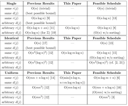
Previous Results We review the current fastest algorithms for nine scheduling problems discussed in this paper. The summary is given in Table 1.
Single Previous Results This Paper Feasible Schedule same r(j) O(n) (trivial) — O(n) (trivial) same d(j) (best possible bound)
same r(j) O(nlogn) [9] — O(nlogn) [13] arbitraryd(j) (best possible bound)
arbitraryr(j) O(nlogn+κn) [11] O(nlogn) O(nlogn) [8] arbitraryd(j) O(nlogn) (forZ) [19] (O(n) w/o sorting)
Identical Previous Results This Paper Feasible Schedule
same r(j) O(n) [17] — O(n) [13]
same d(j) (best possible bound)
same r(j) O(n2(logn)2) [12] O(nlogmlogn) O(nlogn) [15]
arbitraryd(j) (O(nlogm) w/o sorting)
arbitraryr(j) O(n2(logn)2) [12] — O(n2(logn)2) (cf. [2, 21])
arbitraryd(j)
Uniform Previous Results This Paper Feasible Schedule same r(j) O(mn+nlogn) [14] O(min{nlogn, O(mlogm+n) [6] same d(j) n+mlogmlogn})
same r(j) O(mn3) [12] O(mnlogn) O(mn+nlogn) [16]
arbitraryd(j) (O(mn) w/o sorting)
arbitraryr(j) O(mn3) [12] — O(mn3) [3]
[image:5.595.79.512.97.456.2]arbitraryd(j)
Table 1: Summary of Our Results and Previous Results.
The time complexity with “w/o sorting” means the time complexity except for the time required for sorting input numbers of size O(n) such as w(j), r(j), d(j).
for Single-ArbR-ArbD, which works only for instances with the numbers p(j), p(j), r(j), d(j) given by integers.
Ide-SameR-SameD can be formulated as the continuous knapsack problem by using the result of McNaughton [13], and therefore can be solved in O(n) time (see [17]). McCormick [12] shows that Ide-ArbR-ArbD (and also Ide-SameR-ArbD) can be formulated as a parametric max flow problem, and applies the algorithm of Gallo et al. [5] to achieve the time complexity O(n3logn),
which can be reduced to O(n2(logn)2) by using the balanced binary tree representation of time
intervals as in Chung et al. [2, 21].
Uni-SameR-SameD can be solved by a greedy algorithm in O(mn+nlogn) time [14]. Mc-Cormick [12] shows that Uni-ArbR-ArbD (and also Uni-SameR-ArbD) can be formulated as a parametric max flow problem on a bipartite network, and applies the algorithm of Ahuja et al. [1] to achieve the time complexity O(mn3).
be formulated as a polymatroid optimization problem of the following form:
(LP) Maximize
n
X
j=1
w(j)p(j)
subject to p(Y)≤ϕ(Y) (Y ∈2N), p(j)≤p(j)≤p¯(j) (j∈N),
wherep(Y) =Pj∈Y p(j) andϕ: 2N →
R+is a polymatroid rank function, i.e., a nondecreasing
submodular function withϕ(∅) = 0. This observation is already made in [12, 17, 18] and used to show the validity of greedy algorithms for the scheduling problems. On the other hand, we use this observation in a different way; we develop a novel divide-and-conquer technique for the problem (LP), and apply it to the scheduling problems to obtain faster algorithms.
We define a functionϕe: 2N →Rby
e
ϕ(X) = min
Y∈2N{ϕ(Y) +p(X \Y)−p(Y \X)} (X ∈2
N).
Then,ϕe is also a polymatroid rank funciton, and the set of maximal feasible solutions of (LP) is given as {p ∈Rn | p(Y) ≤ϕe(Y) (Y ∈ 2N), p(N)=ϕe(N)} (cf. [4, Sect. 3.1(b)]). Our
divide-and-conquer technique is based on the following property, where the proof is given in Sect. 2:
Theorem 1.1. Let k ∈N and Nk={j∈N |w(j)≥w(k)}. Suppose that X∗ ∈2N satisfies
e
ϕ(Nk) =ϕ(X∗) +p(Nk\X∗)−p(X∗\Nk). (1.1)
Then, there exists an optimal solution q ∈ Rn of the problem (LP) satisfying q(X∗) = ϕ(X∗), q(j) =p(j) (j∈Nk\X∗), and q(j) =p(j) (j∈X∗\Nk).
By Theorem 1.1, the problem (LP) can be decomposed into two subproblems of similar structure, where the one is with respect to the variables {p(j) | j ∈ X∗} and the other with respect to{p(j)|j ∈N \X∗}. Moreover, Theorem 1.1 shows that some of the variables can be fixed, which implies that each of the two subproblems contains at most n/2 non-fixed variables if we choose k = n/2. Hence, we can show that the depth of recursion is O(logn) when this decomposition technique is applied recursively to (LP).
We also show that a subset X∗ ∈ 2N satisfying (1.1) can be computed in O(Tfeas(n)) time
for each of the scheduling problem, where Tfeas(n) denotes the time complexity for computing
a feasible schedule withn jobs, except for the time required for sorting the input numbers (see Table 1 for the actual time complexity for comptuing a feasible schedule). This implies that each scheduling problem can be solved in O(Tfeas(n)×logn) time by using our divide-and-conquer
technique. By applying this approach, we can obtain faster algorithms for four of the nine scheduling problems discussed in this paper (see Table 1).
2
Divide-and-Conquer Technique for Polymatroid Optimization
We explain our divide-and-conquer technique for the problem (LP). The discussion in this section is based on basic properties of polymatroids and submodular polyhedra (see, e.g., [4]).
We, without loss of generality, assume that the weights w(j) (j ∈ N) are all distinct; this assumption can be easily fulfilled, e.g., by using perturbation. In addition, we suppose that a subsetF ⊆ N such that p(j) =p(j) (j ∈F) is given, i.e, the variable p(j) for each jobj ∈ F is already fixed. The set F is called a fixed-job set, and will be used in the divide-and-conquer algorithm. We denote by ˆnthe number of non-fixed variables in (LP), i.e., ˆn=n− |F|.
We first show how to decompose the problem (LP) into subproblems. Let k ∈ N be an integer with|Nk\F|=bn/ˆ 2c, whereNk={j∈N |w(j)≥w(k)}. Suppose that (1.1) holds for
some X∗ ∈2N. By Theorem 1.1, the problem (LP) can be decomposed into the following two subproblems of smaller size:
(SLP1) Maximize Pj∈X∗w(j)p(j)
subject to p(Y)≤ϕ1(Y) (Y ∈2X∗),
p(j)≤p(j)≤p¯(j) (j∈X∗∩Nk), p(j) =p(j) (j ∈X∗\Nk),
(SLP2) Maximize Pj∈N\X∗w(j)p(j)
subject to p(Y)≤ϕ2(Y) (Y ∈2N\X∗),
p(j)≤p(j)≤p¯(j) (j∈(N \Nk)\X∗), p(j) =p(j) (j∈Nk\X∗),
whereϕ1 : 2X∗ →R and ϕ2 : 2N\X∗ →Rare defined as
ϕ1(Y) =ϕ(Y) (Y ∈2X∗), ϕ2(Y) =ϕ(Y ∪X∗)−ϕ(X∗) (Y ∈2N\X∗).
Note that the subproblems (SLP1) and (SLP2) (and their corresponding scheduling problems) have a structure similar to that of the original problem (LP).
Lemma 2.1. Suppose that p1 ∈ RX∗ (resp., p2 ∈ RN\X∗) is an optimal solution of (SLP1)
with p1(X∗) = ϕ1(X∗) (resp., (SLP2) with p2(N \X∗) = ϕ2(N \X∗)). Then, the direct sum p=p1⊕p2 ∈Rn of p1 and p2 defined by
(p1⊕p2)(j) =
(
p1(j) (j∈X∗), p2(j) (j∈N\X∗)
is an optimal solution of(LP) with p(N) =ϕ(N).
The fixed-job sets for (SLP1) and (SLP2) are given by F1 = (F ∩X∗)∪(X∗ \Nk) and
F2 = (F \X∗)∪(Nk\X∗), respectively. Since
|X∗\F1| ≤ |Nk\F|=bn/ˆ 2c, |(N\X∗)\F2| ≤ |(N\Nk)\F| =dn/ˆ 2e, (2.1)
We then explain how to computeX∗ ∈2N satisfying (1.1). We have
e
ϕ(Nk) =−p(N\Nk) + min
X∈2N{ϕ(X) +p(Nk\X) +p((N \Nk)\X)}, (2.2)
and the second term in the right-hand side of (2.2) is equal to the optimal value of the following problem (cf. [4, Sect. 3.1 (b)]):
(ULP) Maximize
n
X
j=1 p(j)
subject to p(X)≤ϕ(X) (X ∈2N), 0≤p(j)≤u(j) (j∈N),
where
u(j) = (
p(j) (j∈Nk),
p(j) (j∈N\Nk).
(2.3)
The problem (ULP) is a special case of the problem (LP) where the objective function is un-weighted, i.e., w(j) = 1 (j ∈N), and the lower bound of the variable p(j) (j ∈N) is equal to zero, and therefore easier to solve. The scheduling problem corresponding to (ULP) is to max-imize the sum of processing requirements under the upper bound constraint and the feasibility constraint that the processing requirements can be feasibly scheduled on machines, and can be solved in O(Tfeas(n)) time, in a similar way as the problem of computing a feasible schedule.
Let q ∈ Rn be an optimal solution of (ULP), and X∗ ∈ 2N the unique maximal set with q(X∗) = ϕ(X∗). It is shown in the following sections that such X∗ can be computed in O(Tfeas(n)) time. By the optimality ofq and submodularity of ϕ, we have
q(j) =p(j) (j∈Nk\X∗), q(j) =p(j) (j∈(N\Nk)\X∗)),
implying thatX∗ satisfies (1.1) since
e
ϕ(Nk) = −p(N \Nk) +q(N)
= −p(N \Nk) +{ϕ(X∗) +p(Nk\X∗) +p((N \Nk)\X∗)}
= ϕ(X∗) +p(Nk\X∗)−p(X∗\Nk).
Finally, we analyze the time complexity of our divide-and-conquer algorithm. Let T(n,nˆ) be the time complexity for solving the problem (LP) withnvariables and ˆnnon-fixed variables, except for the time required for sorting input numbers. Then, we have
T(n,ˆn) = O(Tfeas(n)) +T(n1, n01) +T(n2, n02),
where n1 +n2 = n, n10 ≤min{n1,bn/ˆ 2c}, and n02 ≤ min{n2,dn/ˆ 2e}. By solving the recursive
equation, we haveT(n,ˆn) = O(Tfeas(n)×logn).
Theorem 2.2. Suppose that a subset X∗ ∈2N satisfying (1.1) can be computed in O(Tfeas(n))
Finally, we give a proof of Theorem 1.1.
Proof of Theorem 1.1. Since the set of maximal feasible solutions of (LP) is given as {p∈Rn|
p(Y) ≤ϕe(Y) (Y ∈ 2N), p(N)=ϕe(N)}, the vector p∗ ∈ Rn given by p∗(j) =ϕe(N
j)−ϕe(Nj−1)
(j = 1,2, . . . , n) is an optimal solution of (LP) (cf. [4, Sect. 3.1]). We show that the vector q=p∗ satisfies the conditions
q(X∗) =ϕ(X∗), q(j) =p(j) (j∈Nk\X∗), q(j) =p(j) (j∈X∗\Nk). (2.4)
Sincep∗ is a feasible solution of the problem (LP), we have
p∗(X∗)≤ϕ(X∗), p∗(j)≤p(j) (j∈Nk\X∗), −p∗(j)≤ −p(j) (j∈X∗\Nk). (2.5)
By the definition ofp∗, we have p∗(N
k) = ϕe(Nk) = ϕ(X∗) +p(Nk\X∗)−p(X∗\Nk), which,
together with (2.5), implies that all the inequalities in (2.5) hold with equality. Hence, (2.4) follows.
3
Single Machine with Arbitrary Release/Due Dates
We apply the divide-and-conquer technique in Sect. 2 to the problem Single-ArbR-ArbD. To describe the algorithm, we consider a restriction on the availability of the machine. Let ˜I =
{[gk, gk+1]|k = 1,2, . . . ,2n−1} be a set of time intervals, where gk is thek-th largest number
in{r(j), d(j)|j∈N}. We are given a set of time intervalsI ={[e1, f1],[e2, f2], . . . ,[e`, f`]} ⊆I˜
such that the machine is available only in these time intervals, wheree1 ≤f1 ≤ · · · ≤e` ≤f`.
In addition, we are given a subsetF of jobs (fixed-job set) such thatp(j) =p(j) forj∈F. We denote this variant of the problem Single-ArbR-ArbD by P(I, N, F). Any subproblem which appears during the recursive decomposition of the problem Single-ArbR-ArbD is of the form P(I, N, F); in particular, the original problem Single-ArbR-ArbD coincides with P( ˜I, N,∅).
The problem P(I, N, F) can be formulated as the problem (LP) with the polymatroid rank functionϕ: 2N →Rgiven by
ϕ(X) =X{fk−ek|1≤k ≤`, [ek, fk]⊆[r(j), d(j)] for somej∈X}.
Let k ∈ N be an integer with |Nk\F| = bn/ˆ 2c, where ˆn = n− |F|, and suppose that X∗ ∈ 2N satisfies (1.1). Then, P(I, N, F) is decomposed into the subproblems P(I
1, N1, F1) and
P(I2, N2, F2), where
I1={[ek, fk]|1≤k≤`, [ek, fk]⊆[r(j), d(j)] for some j∈X∗}, N1=X∗, F1= (F ∩X∗)∪(X∗\Nk),
I2=I\I1, N2=N\X∗, F2 = (F \X∗)∪(Nk\X∗).
In addition, we updatep andp by
We decompose the problem P(I, N, F) recursively in this way and compute an optimal solution. We now explain how to computeX∗ ∈2N satisfying (1.1) in O(n) time. It is assumed that the numbersr(j), d(j) (j∈N) andek, fk(k = 1,2, . . . , `) are already sorted. We firstly compute
an optimal solution q ∈ Rn of the problem (ULP) corresponding to P(I, N, F), which can be done in O(Tfeas(n)) = O(n) time by using either of the algorithms in [7, 20]. Then, we compute a
partition{N0, N1, . . . , Nv}ofN such thatq(Nh) = maxj∈Nhd(j)−minj∈Nhr(j) (h = 1,2, . . . , v)
and that N \N0 is maximal under this condition, which can be done in O(n) time. Since
maxj∈Nhd(j) −minj∈Nhr(j) = ϕ(Nh) (h = 1, . . . , v), the set X∗ = N \ N0 is the unique
maximal set withq(X∗) =ϕ(X∗). Hence, Theorem 2.2 implies the following result.
Theorem 3.1. The problem P(I, N, F) can be solved in O(nlogn) time. In particular, the problem Single-ArbR-ArbD can be solved in O(nlogn) time.
It should be mentioned that our algorithm for Single-ArbR-ArbD is similar to the divide-and-conquer algorithm by Shih et al. [19], but the two algorithms are based on different ideas. Indeed, the algorithm in [19] works only for instances with the numbers p(j), p(j), r(j), d(j) given by integers, while ours can be applied to any problem with real numbers.
4
Identical Parallel Machines with the Same Release Dates and
Different Due Dates
We apply the divide-and-conquer technique in Sect. 2 to the problem Ide-SameR-ArbD. To describe the algorithm, we consider a restriction on the availability of the machines. Suppose that we are given numbersbi (i∈M) andcsuch that machineiis available in the time interval
[bi, c]. In addition, we are given a subset F of jobs (fixed-job set) such that p(j) = p(j) for
j ∈ F. We denote this variant of the problem Ide-SameR-ArbD by P(m, B, c, N, F), where B ={bi | i ∈ M}. Any subproblem which appears during the recursive decomposition of the
problem Ide-SameR-ArbD is of the form P(m, B, c, N, F); in particular, the original problem Ide-SameR-ArbD is the case whereb1 =· · ·=bm = 0,c= maxj∈Nd(j), andF =∅.
The problem P(m, B, c, N, F) can be formulated as the problem (LP) with the polymatroid rank functionϕ: 2N →R given by
ϕ(X) =
m
X
i=1
max{min{d(i), c} −bi,0},
where we assume thatb1 ≤b2 ≤ · · · ≤bm and that d(i) is thei-th largest number in{d(j)|j∈
N} for i= 1, . . . , m. Let k ∈N be an integer with |Nk\F| =bn/ˆ 2c, where ˆn=n− |F|, and
suppose that X∗ ∈ 2N satisfies (1.1). Then, the problem P(m, B, c, N, F) is decomposed into the subproblems P(m1, B1, c1, N1, F1) and P(m2, B2, c2, N2, F2), where
m1= min{m,|X∗|}, B1 ={b1, b2, . . . , bm1}, c1 = min{c, d(jm1)}, N1=X∗, F1 = (F ∩X∗)∪(X∗\Nk),
where we assume that{j1, j2, . . . , jm1} ⊆X∗ and that d(ji) is thei-th largest number in{d(j)| j∈X∗}fori= 1, . . . , m1. In addition, we updatep and pby (3.1).
Suppose that p1 ∈ RX∗ (resp., p2 ∈ RN\X∗) is an optimal solution of P(m1, B1, c1, N1, F1)
(resp., P(m2, B2, c2, N2, F2)). Then, the vector p∗∈Rn defined by
p∗(j) = (
p1(j) + max{0, d(j)−d(jm1)} (j∈X∗), p2(j) (j∈N \X∗)
is an optimal solution of P(m, B, c, N, F).
We now explain how to computeX∗ ∈2N satisfying (1.1) in O(nlogm) time. It is assumed that the numbersd(j) (j∈N) are already sorted. By using a slight modification of the algorithm by Sahni [15], we can compute an optimal solutionq∈Rn of the problem (ULP) corresponding to P(m, B, c, N, F) in O(Tfeas(n)) = O(nlogm) time. Then, we compute the unique maximal
setX∗ ∈2N withq(X∗) =ϕ(X∗). Using the following simple observations, we can find suchX∗ in O(nlogm) time.
Lemma 4.1.
(i) {j∈N |p(j)< u(j)} ⊆X∗.
(ii) Let j ∈X∗ and j0 ∈N \ {j}. Suppose that there exists a time interval [e, f] satisfying the following conditions: [e, f] ⊆ [r(j), d(j)], any portion of job j is not processed on [e, f], and some portion of job j0 is processed on [e, f]. Then, we have j0∈X∗.
Theorem 4.2. The problem P(m, B, c, N, F) can be solved in O(nlogmlogn) time. In partic-ular, the problem Ide-SameR-ArbD can be solved in O(nlogmlogn) time.
We can solve the problem Uni-SameR-ArbD in a similar way as Ide-SameR-ArbD by using the algorithm of Sahni and Cho [16]. The details of the proof is omitted.
Theorem 4.3. The problem Ide-SameR-ArbD can be solved in O(mnlogn) time.
5
Uniform Parallel Machines with the Same Release/Due Dates
We apply the divide-and-conquer technique in Sect. 2 to the problem Uni-SameR-SameD. For the description of the algorithm, we consider the problem Uni-SameR-SameD with a subsetF ob jobs (fixed-job set) such thatp(j) =p(j) forj∈F. We denote this problem by P(M, N, F), whereM andN denote the sets of machines and jobs, respectively. Note that P(M, N,∅) coincides with the original problem Uni-SameR-SameD. It is assumed that the speed of machines are already sorted and satisfys1 ≥s2≥ · · · ≥sm.
5.1 The First Algorithm
The problem P(M, N, F) can be formulated as (LP) with the polymatroid rank function ϕ : 2N → R given by ϕ(X) =dS
min{m,|X|} (X ∈2N), where Sh =
Ph
be decomposed (or reduced) into subproblems of smaller size, as follows. We assume that the numbers{p(j)|j∈N} ∪ {p(j)|j∈N}is already sorted.
The next property is a direct application of Theorem 1.1 to the problem P(M, N, F).
Lemma 5.1. Letk ∈N, and suppose thatX∗ ∈2N satisfies(1.1). Then, there exists an optimal solutionq ∈Rn of the problem P(M, N, F) satisfying the following properties, where h=|X∗|: (i) if h < m, then q(X∗) =dSh, q(j) =p(j) (j∈Nk\X∗), q(j) =p(j) (j ∈X∗\Nk).
(ii)If h≥m, then q(N) =dSm and q(j) =p(j) (j ∈N \Nk).
Letk ∈N be an integer with|Nk\F|=bn/ˆ 2c, where ˆn=n−|F|, and suppose thatX∗ ∈2N satisfies (1.1). SuchX∗ can be computed in O(n) time by Lemma 5.2 given below.
Lemma 5.2. Suppose that the sorted list of the numbers P ≡ {p(j) | j ∈N} ∪ {p(j) | j∈ N}
is given. For any X ∈2N, we can compute the value of ϕe(X) and a set Y∗ ∈2N with ϕe(X) = ϕ(Y∗) +p(X \Y∗)−p(Y∗\X) in O(n) time.
Leth=|X∗|. Ifh < m, then the problem P(M, N, F) can be decomposed into the following two subproblems P(M1, N1, F1) and P(M2, N2, F2), where
(
M1 ={1,2, . . . , h}, N1 =X∗, F1 = (F ∩X∗)∪(X∗\Nk),
M2 =M\M1, N2=N \X∗, F2= (F \X∗)∪(Nk\X∗).
In addition, we updatep and p by (3.1). Before solving the subproblems, we sort the numbers
P1 ≡ {p(j)|j∈N1} ∪ {p(j) |j∈N1}and P2 ≡ {p(j)|j∈N2} ∪ {p(j)|j∈N2}, which can be
done in O(n) time. Hence, the decomposition can be done in O(n) time.
Ifh≥m, then P(M, N, F) can be reduced to the subproblem P(M1, N1, F1), whereM1=M, N1=N, andF1 =F∪(N\Nk). In addition, we updatepby p(j) :=p(j) (j ∈N\Nk). Hence,
the reduction can be done in O(n) time as well.
The following result follows from Theorem 2.2 and the discussion above.
Theorem 5.3. The problem P(M, N, F) can be solved in O(nlogn) time by the first algorithm. In particular, the problem Uni-SameR-SameD can be solved in O(nlogn) time.
We note that the time complexity of the first algorithm is optimal for Uni-SameR-SameD whenn= O(m) since sorting the speeds of m machines requires O(mlogm) time.
5.2 The Second Algorithm
The running time of the first algorithm is dominated by the time for sorting the numbers inP. To reduce the time complexity, we modify the first algorithm by using the information of the fixed-job set, so that it does not require the sorted list. We assume that the min{m,|F|}largest numbers in{p(j)|j∈F} and the numberp(F) are given in advance.
Lemma 5.4. Suppose that the min{m,|F|} largest numbers in {p(j)| j ∈F} and the number p(F) = Pj∈Fp(j) are given. For any X ∈ 2N, we can compute the value of ϕe(X) and a set
Hence, we can computeX∗ ∈2N satisfying (1.1) in O((n− |F|) +mlogm) time. Using the setX∗ we decompose (or reduce) the problem P(M, N, F) into subproblems in the same way as the first algorithm.
If |X∗| < m, then the problem P(M, N, F) can be decomposed into the two subproblems P(M1, N1, F1) and P(M2, N2, F2). The second subproblem P(M2, N2, F2) is solved recursively
by the second algorithm, while the first subproblem P(M1, N1, F1) is solved by the first
algo-rithm in O(|M1|log|M1|) = O(mlogm) time. Before solving P(M2, N2, F2), we compute the
min{m,|F2|} largest numbers in {p(j) | j ∈ F2} and the number p(F2), which can be done in
O((n− |F|) +mlogm) time.
If |X∗| ≥ m, the problem P(M, N, F) is reduced to the subproblem P(M1, N1, F1), which
is recursively solved by the second algorithm. Before solving the subproblem, we compute the min{m,|F1|} largest numbers in {p(j) | j ∈ F1} and the number p(F1), which can be done in
O((n− |F|) +mlogm) time as well.
LetT2(m, n,nˆ) denote the running time of the second algorithm for P(M, N, F). Then, the
following recursive formula holds:
T2(m, n,nˆ) =
O(mlogm) (if ˆn≤1),
O(ˆn+mlogm) +T2(|M2|,|N2|,|N2| − |F2|) (if ˆn≥2, |X∗|< m), O(ˆn+mlogm) +T2(|M1|,|N1|,|N1| − |F1|) (if ˆn≥2, |X∗| ≥m).
Note that|N2| − |F2| ≤ dn/ˆ 2e and |N1| − |F1| ≤ bn/ˆ 2c by (2.1). Hence, we have T2(m, n,nˆ) = O(ˆn+mlogmlog ˆn). As a preprocessing, we need to compute the min{m,|F|}largest numbers in{p(j)| j∈F}and the numberp(F), which requires O(n+mlogm) time. Hence, the following result holds.
Theorem 5.5. The problemP(M, N, F)can be solved inO(n+mlogmlogn)time by the second algorithm. In particular,Uni-SameR-SameD can be solved in O(n+mlogmlogn) time.
References
[1] R. K. Ahuja, J. B. Orlin, C. Stein, R. E. Tarjan, Improved algorithms for bipartite network flow, SIAM Journal on Computing23 (1994), 906–933.
[2] J. Y. Chung, W.-K. Shih, J. W. S. Liu, and D. W. Gillies, Scheduling imprecise computa-tions to minimize total error, Microprocessing and Microprogramming 27 (1989), 767–774.
[3] A. Federgruen and H. Groenevelt, Preemptive scheduling of uniform machines by ordinary network flow techniques, Management Science32 (1986), 341–349.
[4] S. Fujishige, Submodular Functions and Optimization, Second Edition, Annals of Discrete Mathematics 58, Elsevier, 2005.
[6] T. F. Gonzales and S. Sahni, Preemptive scheduling of uniform processor systems,Journal of ACM 25 (1978), 92–101.
[7] D. S. Hochbaum and R. Shamir, Minimizing the number of tardy job unit under release time constraints, Discrete Applied Mathematics 28 (1990), 45–57.
[8] W. Horn, Some simple scheduling algorithms,Naval Res. Logist. Quat.21 (1974), 177–185.
[9] A. Janiak and M.Y. Kovalyov, Single machine scheduling with deadlines and resource de-pendent processing times, European Journal of Operational Research 94 (1996), 284–291.
[10] J. Y.-T. Leung, Minimizing total weighted error for imprecise computation tasks and related problems, Chapter 34 of Handbook of Scheduling (ed.: J. Y-T. Leung), Chapman & Hall, 2004, 34-1–34-16.
[11] J. Y.-T. Leung, V. K. M. Yu, and W.-D. Wei, Minimizing the weighted number of tardy task units, Discrete Applied Mathematics51 (1994), 307–316.
[12] S. T. McCormick, Fast algorithms for parametric scheduling come from extensions to para-metric maximum flow, Operations Research 47 (1999), 744–756.
[13] R. McNaughton, Scheduling with deadlines and loss functions, Management Science 12 (1959), 1–12.
[14] E. Nowicki and S. Zdrza lka, A bicriterion approach to preemptive scheduling of parallel machines with controllable job processing times, Discrete Appl. Math. 63 (1995), 237–256.
[15] S. Sahni, Preemptive scheduling with due dates,Operations Research 27 (1979), 925–934.
[16] S. Sahni and Y. Cho, Scheduling independent tasks with due times on a uniform processor system, Journal of the ACM27 (1980), 550–563.
[17] N. V. Shakhlevich and V. A. Strusevich, Pre-emptive scheduling problmes with controllable processing times, Journal of Scheduling 8 (2005), 233–253.
[18] N. V. Shakhlevich and V. A. Strusevich, Preemptive scheduling on uniform parallel ma-chines with controllable job processing times, Algorithmica, to appear.
[19] W.-K. Shih, C.-R. Lee, and C.-H. Tang, A fast algorithm for scheduling imprecise compu-tations with timing constraints to minimize weighted error, Proceedings of the 21th IEEE Real-Time Systems Symposium (RTSS2000) (2000), 305–310.
[20] W.-K. Shih, J. W. S. Liu, and J.-Y. Chung, Algorithms for scheduling imprecise computa-tions with timing constraints, SIAM Journal on Computing 20 (1991), 537–552.
Appendix
A
Proofs
A.1 Proof of Lemma 2.1
Lemma 2.1 is immediate from the following proposition and the fact that there exists an optimal solutionq ∈Rn of (LP) withq(X∗) =ϕ(X∗).
Proposition A.1 (cf. [4, Lemma 3.1]). Suppose that p1 ∈ RX∗ (resp., p2 ∈ RN\X∗) is a
feasible solution of(SLP1) withp1(X∗) =ϕ1(X∗)(resp., (SLP2)withp2(N\X∗) =ϕ2(N\X∗)). Then, the direct sum p=p1⊕p2∈Rn of p1 and p2 defined by
(p1⊕p2)(j) =
(
p1(j) (j∈X∗), p2(j) (j∈N\X∗)
is a feasible solution of(LP)with p(N) =ϕ(N). Conversely, for any feasible solutionp∈Rnof (LP) satisfying p(X∗) =ϕ(X∗), the restriction of p on X∗ (resp., on N \X∗) yields a feasible solution of(SLP1) with p1(X∗) =ϕ1(X∗) (resp., (SLP2) with p2(N\X∗) =ϕ2(N \X∗)).
A.2 Proof of Lemma 5.2
Recall that the function ϕ : 2N → R is given by ϕ(Y) = dS
min{m,|Y|} (Y ∈ 2N) and the function value ofϕ(Y) depends only on the cardinality ofY. For i= 1,2, . . . , m−1 we denote
Fi ={Y ∈2N | |Y|=i}. Since pand p are nonnegative vectors, it follows from (2.2) that
e
ϕ(X) = −p(N \Nk) + min
Y∈2N{ϕ(Y) +p(X\Y) +p((N \X)\Y)}
= −p(N\X) + minϕ(N), min
Y∈∪m−1 i=1 Fi
{ϕ(Y) +p(X \Y) +p((N \X)\Y)}
= −p(N\X) + min
dSm, min
0≤i≤m−1
dSi+ min Y∈Fi
{p(X \Y) +p((N \X)\Y)}
= −p(N\X) + min
dSm, min
0≤i≤m−1
dSi+p(X) +p(N \X)
−max
Y∈Fi
{p(X∩Y) +p((N \X)∩Y)}
. (A.1)
For i = 1,2, . . . , m, we denote by αi the i-th largest number in the set PX ≡ {p(j) | j ∈
X} ∪ {p(j) | j ∈ N \X}. By using the sorted list of P, the values α1, α2, . . . , αm can be
computed in O(n) time. Then, we have
max
Y∈Fi
{p(X ∩Y) +p((N \X)∩Y)}=
i
X
k=1 αk.
Hence, the value ϕe(X) can be computed in O(n) time by using the formula above. If the minimum in the RHS of (A.1) is attained bydSm, then we can choose Y∗ =N; otherwise, we can choose Y∗ ={j1, j2, . . . , jk}, where jk∈N (k = 1,2, . . . , m) is the number withαk =p(jk)
A.3 Proof of Lemma 5.4
We prove the claim in a similar way as that for Lemma 5.2. Since
PX ={p(j)|j∈X\F} ∪ {p(j)|j ∈(N \X)\F} ∪ {p(j)|j∈F}