Material implication of Chile’s economic growth: combining material flow accounting (MFA) and structural decomposition analysis

promoting access to White Rose research papers

White Rose Research Online

Universities of Leeds, Sheffield and York

http://eprints.whiterose.ac.uk/

This is an author produced version of a paper published in Ecological

Economics.

White Rose Research Online URL for this paper:

http://eprints.whiterose.ac.uk/4806/

Published paper

Muñoz, P. and Hubacek, K. (2007)

Material implication of Chile’s economic

growth: combining material flow accounting (MFA) and structural

Material implication of Chile’s economic growth: combining material flow

accounting (MFA) and structural decomposition analysis (SDA)*

Pablo Muñoz J.

Klaus Hubacek

a

Institute of Environmental Science and Technology, Autonomous University of Barcelona, Spain.

b

Sustainability Research Institute (SRI), School of Earth and Environment, University of Leeds, UK

Over the last three decades, the economic integration of the Chilean economy into global markets has happened at a fast pace. For example, in 1986, exports represented 29% of GDP while in 1996 they had increased to 38% of GDP. This period of time was characterized by strong economic growth with an average annual growth rate of about 10%. From a physical perspective, material requirements more than doubled from 220 to 500 million tons of direct material inputs (DMI) during the same decade (the rate of material growth requirements was around 13% per year).

The main objective of this study is to explain the changes in DMI by using a Structural Decomposition Analysis (SDA). The changes in material flow accounting (MFA) were broken down into the effects caused by changes in resource use per unit of output (material intensity effect), changes between and within sectors (structural change effect), changes in the composition of final demand (mix effect), changes due to shifting shares of domestic final demand and exports categories (category effect) and finally changes in the overall level of economic activities (level effects). The results, as percentage of the total level of DMI used in 1986, indicate that economic growth was the major source of material changes (109%). The material intensity and category effects explained 31% and 14% of the increase, respectively. The increase in the material intensity is mainly due to a declining quality of ores in copper production. However, these components were partly compensated by the structure (-14%) and mix (-13%) effects. Therefore, for a Southern American country such as Chile, the main causes of these changes in material consumption have been a combination of the nature of economic growth, increases in export production and increasing material intensity of production.

Keywords: Material Flow Analysis (MFA); Structural decomposition analysis (SDA); input-output analysis; economic growth; international trade; Chile.

a

Corresponding author. Tel.: +44 113 343 1631.

E-mail address:

[email protected]

1 Introduction

Since the end of the 1960s, socio-economic systems have been studied as open systems

which are embodied in a wider physical system, the environment (Ayres, 1969;

Georgescu-Roegen, 1971; Boulding, 1973

metaphorically, as living organisms. Industrial economies ‘ingest’ raw materials, which are

“metabolized” to produce goods and services, and they ‘excrete’ wastes in the form of discarded

materials and pollution” (Matthews et al., 2000, p.1). The study of exchange relationships of

material and energy between socio-economic systems and the environment has been referred to

as ‘industrial metabolism’ (Ayres et al., 1994) or ‘society’s metabolism’ (Fischer-Kowalski,

1998). In spite of the relatively early ideas by Ayres, only recently, in the 1990s, has

considerable progress been made with regards to accounting of materials used by economies

(see for example Adrianse, 1997 or Schandl, 1998). More recently, have standardized and

harmonised relevant concepts emerged providing a comprehensive framework for

economy-wide material flow accounts and analysis (MFA) and material balances Eurostat (2001) 1.

The underlying concept of the material-based approach is the mass balance principle.

This principle establishes that all ‘inputs’ going into the economy and coming from the

environment will return, sooner or later, to the environment in the form of waste and emissions.

On the one hand, all materials relate either to some form of scarcity of resources or a rate of

regeneration or renewal. On the other hand, many environmental impacts are caused by material

extraction, throughout the production processes, final consumption, and after disposal. Thus, the

‘strength of an economy-wide MFA is that it provides a comprehensive and consistent picture

of the quantity and composition of the metabolism of economies’ (Bringezu, et al., 2003, p. 47);

a weakness has been its ignorance of qualitative differences of various material flows and the

explicit link to environmental damage (which is assumed rather than factually established).

However, one of the key issues when studying societal (industrial) metabolism is how

the different socio-economic systems exchange materials and energy between them, specifically

how environmental goods as well as the environmental loads are distributed amongst different

systems. A significant part of the literature has focused especially on the north-south

relationship. According to this theory, the Southern countries provide the material and energy

requirements for Northern countries to maintain and develop their socio-economic metabolism

(Muradian and Martinez-Alier, 2001a, Giljum and Eisenmenger, 2004 and Perez, 2006). At the

same time, the materials and energy imported by Northern countries often embody (or cause)

large quantities of emissions and waste which remain in the exporting, usually Southern,

countries (Muradian and Martinez-Alier, 2001b). A clear example of this situation is copper ore

extraction: given the low copper content in minerals (around 1%), it is necessary to extract huge

ore quantities in order to obtain a certain amount of pure copper output to be used in the

economic process. We should note that Chile is the first copper supplier in the world (around

36% of the world market), with an output of 5.3 million tons of copper in 2006 (Procobre,

2006).

Some authors (Hornborg, 1998, Perez, 2006) have commented on how this

appropriation of natural resources and the burden reallocation are related to different

mechanisms such as prices, direct foreign investment and international trade, which facilitate

natural resource extraction. These mechanisms have clear effects on the economic structure.

Thus, having a comprehensive view of the dynamics of the economic structure is an important

precondition when studying changes in material use. Hence, considering changes in the

economic structure over time that govern material flows between producing industries,

consuming households and exports is indispensable for solving the problems of both limited

resource availability and pollution (Suh and Kagawa, 2005).

Therefore, the objective of this study is to analyse the driving forces of material

consumption in Chile over the time period of 1986 to 1996. We will mainly stress the effects of

international trade and economic growth on environmental pressures. The analysis of these

drivers, among others, gives us a comprehensive view about the material use during the

observed time period in Chile, describing the material implications of changes in Chile’s

In the next sections we proceed as follows: section two provides the economic context

of Chile in terms of trade liberalization as well as a review of previous important work on

material use. In section three we present the methodology for analyzing the socio-economic

changes in Chile by employing a structural decomposition analysis. In section four we present

2 The Chilean case: antecedents

2.1 The economic perspective

Over the last three decades, one could observe an intensifying economic integration of

the Chilean economy into global markets. During the same time period Chilean economic

policies have emphasised economic stabilization and liberalization; for example a reduction of

import tariffs from 105% in 1974 to a uniform tariff of 10% set in 1979 (Corbo and de Melo,

1987). During the 1990s, these policies were reinforced in the direction called for by the

“Washington Consensus2” which is a “summary of the lowest common denominator of policy

advice addressed by the Washington based institutions (including the World Bank) to Latin

America” (Williamson, 2000, p. 251). Some of these policies considered in the “Washington

Consensus” were: trade liberalization, liberalization of inflows of foreign direct investment,

privatization, deregulation (to abolish barriers to entry and exit), and secure property rights,

amongst others. Thus, in order to continue the trade liberalization path during this time period

many free trade agreements took place between Chile and Canada (1996), the European Union

(2002), the United States (2003), South Korea (2003), New Zealand, Singapore and Brunei

Darussalam (2005) and other complimentary economic agreements with Latin American

countries. Current negotiations are with China, Japan and India. Thus, exports as a percentage

of GDP rose from 10% in 1973 to 40% in 2000 (Banco Central de Chile, 2001a). Today, Chile

is widely recognized as having the most open, stable, and liberalized economy in Latin America

(World Bank, 2001). In spite of achieved stabilization and economic growth there are a number

of critical voices reflecting on social3 and ecological dimensions (Quiroga and Van

Hauwermeiren, 1996, Altieri and Rojas, 1999, Larrain et al., 2003).

See for example Williamson (1990).

3

2.2 The physical perspective

In the last decade, the awareness about national level material consumption has

significantly increased. A recent EU-funded project (MOSUS4) provides estimations of

domestic extraction5 for all world regions and many of the world’s economies (Behrens et al.,

2005). The MOSUS data shows that the richest countries6, which represented in 2000 14% of

the world’s population and 75% of the world’s GPD, have extracted 34% of the world’s

materials. This means, of course, that the rest of the countries have extracted 66% of the direct

material inputs, but have just generated 25% of the GDP for 86% of the world’s population.

From a conventional economic point of view these figures could be mainly explained by

theories such as ‘comparative advantage’ referring to different levels of capital accumulation

and availability of qualified labour in the richest countries. In the words of the world-system

perspective, the ‘global order’ and their inherent properties such as prices, different economic

structures and trade relationships lead to a progressive spatial separation of extraction,

production and consumption. As a consequence, an uneven distribution of physical material use

between the rich and poor countries (or core versus periphery) takes place (see Hornborg et al.,

2007; Bunker, 2007).

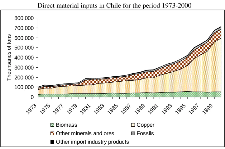
Especially relevant for the case of Chile are MFA estimations by Giljum (2004)

provided for the time period of 1973 to 2000. Figure 1 gives an overview of the use of different

material categories for the last three decades showing an especially rapid increase in material

use during the 1990s. This was mainly due to DMI triggered by resource-intensive exports from

mining, fruit planting, forestry and fishery sectors.

A data base about MOSUS ((Modelling opportunities and limits for restructuring Europe towards sustainability) project results can be found at www.materialflows.net.

5

Domestic extraction is defined as all solid, liquid and gaseous materials (excluding water and air but including e.g. the water content of materials) that enter the economy for further use in production or consumption processes. If it is added the material imports, then we obtain the Direct Material Input (DMI) indicator, which is equal to domestic extraction (DE) of material plus imports (Eurostat, 2001).

6

0 100,000 200,000 300,000 400,000 500,000 600,000 700,000 800,000 197 3 197 5

1977 197 9 198 1 198 3 198 5

1987 198 9 199 1 199 3 199 5

1997 199 9 T h o uns and s of ton s

Biomass Copper Other minerals and ores Fossils

Other import industry products

Figure 1

Direct material inputs in Chile for the period 1973-2000

Source: Giljum 2004.

Note: Each material category includes domestic extraction and imports

into the system.

Furthermore, we would like to highlight that most of the materials incorporated into the

Chilean economy were required to produce exports. Using a static input-output approach results

have shown that the Chilean exports caused around 80% of the DMI in 1996 (Muñoz and Roca,

2006). This approach not only considered those materials which were physically exported but

also those direct materials that were necessary to produce exports.

So far, we have briefly described some physical, monetary and geopolitical position

from this economy of the South. In the next section we present the methodology to study the

3 Methodology

3.1 Structural Decomposition Analysis

Structural Decomposition Analysis (SDA) has widely been applied during the last three

decades; the first formal derivation is attributed to Leontief and Ford (1972). SDA is used to

explain the changes that occur in any variable over the time or space7. This technique has

frequently been utilized to tackle topics related to the environment. For example, it has

frequently been applied to energy (Lin and Polenske 1995, Mukhopadhyay, 1999, Jacobsen,

2000) and air pollution emissions (Casler and Rose, 1998, Wier, 1998, Haan, 2001,

Mukhopadhyay and Forssel, 2005, and Roca and Serrano, 2006). Also, it is possible to find

SDA application to others kinds of materials, for example, nitrogen (Wier and Hasler 1999).

The most recent comprehensive summary has been provided by Hoektra8 (2005) who, among

others, also applied SDA to analyse the flows of iron and steel and plastics for the Netherlands.

However, in spite of the increasing use and relevance of MFA over the last fifteen years, we just

found one study combing SDA and MFA (see Moll et al., 1998).

We can describe SDA as decomposing the change of a variable over, at least, two points

in time (or space). In order to do this, we have decomposed the variable under study according

to our research objective. In a second stage, we take IO tables for two points in time to obtain

the different component contributions (driving forces) to changes in material consumption

between the two measurements.

3.2 The model

In a particular time period t the materials used by the economy can be written as

follows:

M = mq’ × q (1)

assuming a disaggregation of n commodities; M (1x1) are the amount of materials used by the

socio-economic system in period t; the vector q (nx1) represents n commodities; mq’ (1xn)

SDA has also been used for a spatial analysis; see for example, Alcántara et al. (2004).

8

represent the transposed vector of direct materials intensities which represent the materials used

in each sector m per unit of output. Additionally, q can be replaced by the well-known Leontief

inverse (I-A)-1 times final demand y:

M = mq’× (I – A) -1 ×y = mq’×L×y (2)

Where: ‘y’ (nx1) correspond the vector of final demand by commodity; I (mxm) is the identity

matrix; A (mxm) is the matrix of technical coefficient commodity-by-commodity and (I – A)-1 is

the Leontief inverse L which allows capturing direct and indirect effects triggered through

changes in final demand (y), such as exports, government or household demand.

Therefore equation 2 expresses total, direct and indirect, quantities of materials required

to produce any final demand vector, given direct material intensities and a given economic

structure.

Furthermore, it is possible to break down final demand y in different components9:

y = YMix×YCategory×YLevel or in short y = YM × YC × YL (3)

where YMix is also known as structure or composition effect of final demand, i.e. the percentage

of every commodity in a respective final demand category (household consumption, public

expenditure, exports, etc). The vector Ycategory gives the proportion of every category within

aggregate final demand. Given the study’s objective we have used two categories: the first one

is ‘domestic demand’ including household consumption, public expenditure, investment and

stock change; the second one is ‘exports’. Finally, Ylevel is a scalar which captures the changes in

total volume demanded. Thus, the total decomposition is in the following factors:

M= mq’

×L ×YM × YC × YL (4)

In this second stage, the underlying idea consists of taking into account the differences

between, at least, two time periods in every one of the sources that explains the changes in

materials, while the rest of the potential driving sources (decomposition factors) are kept

constant. Then, we have decomposed for two periods of time (0) and (1) the material according

to the former decomposition already shown in equation 4.

M0 = mq’.L.YM.YC.YL

(5)

M 1= mq’.L.YM .YC.YL

Thus, the difference between the two time periods can be expressed as:

∆M = M1 - M0 = M1 L1 YM1 YC1 YVt- M0 L0 YM0 YC0 YV0L (6)

The difference between periods 1 and 0 can be generated by different possible

combinations of the decomposition under study, in our case 5! (or in the general case n!). As

Dietzenbacher and Los (1998, p.309) commented “there is no reason why one decomposition

should be preferred to the others on theoretical grounds” thus recommending (Mukhopdlyay et

al., 2005; Dietzenbacher and Los, 1998; amongst others) the use of two polar decompositions.

This result should be close to the average of the full set of possible decompositions (5!). Then,

following that procedure, we have considered the first polar decomposition, as usually,

beginning with the final year 1:

∆M = ∆M L1 YM1 YC1 YV1 + M0∆L YM1 YC1 YV1 +

M0 L0∆YM YC1 YV1 +M0 L0 YM0∆YC YV1 + (7)

M0 L0 YM0 YC0∆YV

This implies that the second polar decomposition should be starting with the base year

(‘0’):

∆M = ∆M L0 YM0 YC0 YV0 + M1∆L YM0 YC0 YV0 +

M1 L1∆YM YC0 YV0 + M1 L1 YM1∆YC YV0 + (8)

M1 L1 YM1 YC1∆YV

These are so-called polar images with opposite weights with respect to time, “i.e. base

year (0) versus end year (1) variables, attached to each of the corresponding change factors”

∆M = ½ [∆M L1 YM1 YC1 YV1 + ∆M L0 YM0 YC0 YV0 ] +

½ [M0∆L YM1 YC1 YV1 + M1∆L YM0 YC0 YV0] +

½ [M1 L1∆YM YC0 YV0 + M1 L1∆YM YC0 YV0] + (9)

½ [M0 L0 YM0∆YC YV1 + M1 L1 YM1∆YC YV0] +

½ [M0 L0 YM0 YC0∆YV + M1 L1 YM1 YC1∆YV] +

Where:

∆M: captures the change of the materials used per unit of output. This factor is called material

intensity. Theoretically, it is expected to decrease over time reflecting efficiency gains through

technical change, i.e. less material inputs per unit of outputs.

∆LVt:measures the

change in the commodity input structure

∆YM: identifies changes in the composition of final demand categories.

∆YC:Capture changes between final demand categories;. in this particular case ‘domestic final

demand’ and ‘exports’.

∆YVt measures the changes in total volume of final demand. It can be seen as an economic

growth proxy as it equals changes in GDP.

3.3 Data

The data utilized corresponds to two time periods: 1986 and 1996. It is an interesting

period to analyse given the rapidly increasing rate of resource extraction (see figure 1) alongside

a period of strong economic growth. A more pragmatic reason for this choice is due to the fact

that Chile’s last available monetary input-output table (MIOT) is for 1996. Therefore, the

corresponding materials data was also restricted to this time period.

Monetary IO tables were developed and provided by the Central Bank of Chile (Banco

Central de Chile, 1993 and 2001b). The MIOTs are commodity-by-industry and we have used a

commodity-by-commodity formulation under the industry-technology assumption. Furthermore,

were deflated using the output vector in constant prices available for 26 commodities for the

years 1986 and 1996.

The materials data are based on the estimations made by Giljum (2004) for the two

years under study. We have used direct material input (DMI) as indicator for materials (M) used

and consumed in the economy. It is important to mention that the DMI used in this study does

not take into account water and air. Furthermore, the DMI indicators were disaggregated

according to the commodities provided in the MIOT.

However, with regards to the combination of biophysical and economic data we face a

certain level of uncertainty. We have disaggregated the biophysical data by product according to

products description (see for example Banco Central de Chile 2001a) as proper product

classification, such as ISIC, was not available. Consecutively, we adopted a

commodity-by-commodity formulation in order to account for products produced (or extracted) by a secondary

industry to be allocated on the basis of the primary commodity by using the industry’s

technology assumption10. Another issue worth noting is with regards to the allocation of

material imports; we have allocated physical material imports based on monetary information

coming from the import matrix available in the MIOTs. This does represent an inconsistency to

the idea of extended input-output analysis but is of minor importance in our case. In 1996,

around 68% of the material imports were fossil fuels used by petroleum refineries. That means

that we have reallocated 32% (7 millions of tons) of the products imported, which represent

1,5% of the total DMI using monetary information in 1996 (an analogous procedure was used

for the year 1986).

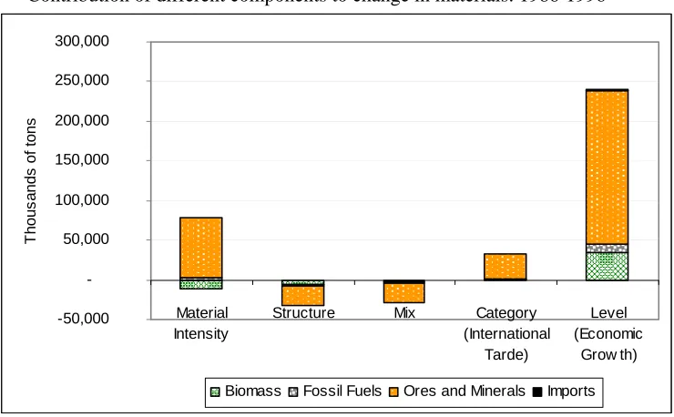
-50,000 -50,000 100,000 150,000 200,000 250,000 300,000 Material Intensity

Structure Mix Category

(International Tarde) Level (Economic Grow th) T h ou s a nds of to ns

Biomass Fossil Fuels Ores and Minerals Imports

4 Results and Discussion

Previous studies on the Chilean socio-economic metabolism have shown that material

requirements have increased from 221 million tons in 1986 to 500 million tons in 1996 (see

Figure 1). In this section we present the contribution of the different components (material

intensity, structure, mix, category and level) by commodity groups to material changes. Figure 2

gives a first overview of the contribution of the different components according to different

kinds of materials. The net addition of the components is equal to the total changes in material

consumption between 1986 and 1996.Furthermore, table 1 gives a comprehensive view on

material changes with regards to the decomposition effects and different commodity groups for

direct material inputs.

Figure 2

Contribution of different components to change in materials: 1986-1996

Note: The total change of direct material inputs was 279 millions, i.e. 500 million tons

in 1996 minus 221 million tons in 1986.

Cod Description M. Intensity Structure Mix Category Level Total M. Intensity Structure Mix Intern. Trade Level Total

1 Agriculture 389 - 1,472 - 1,224 - 61 3,385 1,016 0.18% -0.67% -0.55% -0.03% 1.53% 0.46%

2 Fruit plantation - 233 - 891 258 215 1,918 1,267 -0.11% -0.40% 0.12% 0.10% 0.87% 0.57% 3 Livestock and forestry - 1,520 - 269 - 735 159 4,937 2,573 -0.69% -0.12% -0.33% 0.07% 2.24% 1.17%

4 Fishing - 1,219 - 235 2,093 36 1,115 1,791 -0.55% -0.11% 0.95% 0.02% 0.51% 0.81%

5 Cooper 46,851 - 3,708 - 11,016 26,689 148,721 207,536 21.24% -1.68% -4.99% 12.10% 67.42% 94.09%

6 Other mines 15,560 - 2,269 - 19,531 5,572 29,629 28,962 7.05% -1.03% -8.85% 2.53% 13.43% 13.13%

7 Food, beverages and tobacco - 3,797 - 9,705 - 5,023 28 22,040 3,543 -1.72% -4.40% -2.28% 0.01% 9.99% 1.61% 8 Manufacture of: wearing, dressing, leather and footwear 335 - 836 - 637 - 61 915 - 285 0.15% -0.38% -0.29% -0.03% 0.41% -0.13% 9 Wood products and furniture - 187 852 103 67 1,242 2,078 -0.08% 0.39% 0.05% 0.03% 0.56% 0.94% 10 Manufacture of paper and printing products 103 - 347 - 74 105 902 690 0.05% -0.16% -0.03% 0.05% 0.41% 0.31% 11 Chemical, refined petroleum, rubber and plastic products 2,337 - 6,251 751 - 160 4,712 1,389 1.06% -2.83% 0.34% -0.07% 2.14% 0.63% 12 Other non-metallic mineral products 163 - 15 190 - 3 271 605 0.07% -0.01% 0.09% 0.00% 0.12% 0.27%

13 Basic metals 361 - 519 607 147 925 1,520 0.16% -0.24% 0.28% 0.07% 0.42% 0.69%

14 Metal products, machinery and equipment 533 - 1,282 - 286 - 20 1,315 261 0.24% -0.58% -0.13% -0.01% 0.60% 0.12% 15 Other manufactures industries 16 - 39 36 1 30 45 0.01% -0.02% 0.02% 0.00% 0.01% 0.02% 16 Electricity, gas and water supply 738 - 803 58 - 59 883 818 0.33% -0.36% 0.03% -0.03% 0.40% 0.37%

17 Construction 3,998 1,025 3,988 - 464 7,960 16,506 1.81% 0.46% 1.81% -0.21% 3.61% 7.48%

18 Commerce, hotels and restaurants 1,015 - 1,522 2,313 - 114 3,686 5,378 0.46% -0.69% 1.05% -0.05% 1.67% 2.44%

19 Transport 1,121 - 1,699 325 94 1,837 1,679 0.51% -0.77% 0.15% 0.04% 0.83% 0.76%

20 Communications 40 - 15 113 - 1 82 219 0.02% -0.01% 0.05% 0.00% 0.04% 0.10% 21 Financial intermediation 316 94 - 249 - 37 689 813 0.14% 0.04% -0.11% -0.02% 0.31% 0.37% 22 Activities of private households 335 - 316 - 442 - 51 726 251 0.15% -0.14% -0.20% -0.02% 0.33% 0.11%

23 Education 120 16 - 180 - 24 362 294 0.05% 0.01% -0.08% -0.01% 0.16% 0.13%

24 Health 216 - 526 - 76 - 51 728 290 0.10% -0.24% -0.03% -0.02% 0.33% 0.13%

25 Other service activities 181 - 448 - 131 - 35 493 60 0.08% -0.20% -0.06% -0.02% 0.22% 0.03% 26 Public Administration 488 - 523 - 702 - 82 1,158 339 0.22% -0.24% -0.32% -0.04% 0.52% 0.15%

Total 68,262 - 31,704 - 29,471 31,890 240,662 279,638 30.95% -14.37% -13.36% 14.46% 109.11% 126.78%

As % of DMI used by the economy in 1986 (220.57 millions of material tons) Thounsands of tons

Table 1: Direct material inputs decomposed according to different driving forces and commodity groups for Chile, between the years 1986 and 1996.

The results give us an assessment about the physical dimensions of the driving forces by

commodity group. For the study period, the level effect was the main driver. Note that the level

component can be seen as a proxy variable of ‘economic growth’. Thus, if the Chilean economy

had been grown with the identical levels of material intensity, structure, mix, and category than

it had in 1986 the material use would have increased by 240.66 million tons (or 109% as a

percentage of material used in 1986); Copper (67%), Other mines (13%), Food, beverages and

tobacco (10%), Construction (3,61%), Livestock and forestry (2%) and Chemical, refined

petroleum, rubber and plastic (2%). These commodities together explain 99% of the 109% of

the increase in material use since 1986 (see table 1).

This matches with findings of other studies reporting the level effect as the major

driving force. For example, for the Netherlands, the change of CO2 emissions between the years

1987-1998 was mainly due to the level effect explaining 35% of the change (De Haan 2001). In

the case of Germany, the level component explains 13% of the changes in total material

requirements for the period 1980-1990 (Moll et al., 1998)11.

For the case of Chile the direct material inputs by economic growth (240.66 million

tons) during that time period was larger than the all material required to sustain the

socio-economic metabolism in 1986 (220.57 million tons). In other words, the production level has

more than doubled with a growth rate of around 10% annually. As we have mentioned in

section 2 this has been strongly encouraged by a set of liberalization measures. While GDP was

increasing by this high annual growth rate, the material inputs required to sustain this economic

growth have also increased by about the same rate. Despite the inherent relationship between

economic growth and environmental stress (see for example Arrow et al., 1995) and one to one

link between economic growth and environmental destruction is not given and various extends

of linking and delinking of growth and destruction can be observed for countries during

different development stages and contexts (see the extensive literature on the EKC, e.g. Selden

and Song, 1994; Roca et al., 2001; Seppälä et al., 2001). Thus, the policy context is of

considerable importance - economic policies oriented towards economic growth can lead to an

intensification of resource use, as seen in the case of Chile, if the growth is not accompanied by

appropriate environmental legislation. The policy context is not only important for stirring

economic growth and its environmental implications but for other decomposition elements as

well.

The trend described above has been reinforced by ‘category effects’, which have

contributed 31.89 million tons of material use during this time period. It means that, exports

explain 14% of the change in material consumption. This situation is mainly caused by the

following industries: Copper (12%) and Other mines (2%).

Nevertheless, we would like to highlight that it does not mean that just 31.89 millions of

material tons are necessary to supply to foreign demand. As we have mentioned before, the

Chilean exports caused 80% (399 millions of materials) of the direct material inputs into the

economy in 1996 (Muñoz and Roca, 2006). It is important to note that the “category effect” (or

international trade effect) measures only the change of the share of exports within total final

demand for 1996 with respect to the base year, in this case 189612. The empirical results showed

that the share of exports within final demand increased for the period under study. Thus, the

material consequences of these changes required 31.89 millions of material tons, which is an

increase of 14% in the material consumption as a percentage of material used in 1986.

On the other hand, these effects were partly compensated by ‘mix effects’ due to

changes in final demand composition which decreases the material pressure by 29 million tons

(14% as a percentage of materials used in 1986). The material decrease described by the mix

effect is mainly caused by reduction in the share of Copper, Other mines and Food, beverages

and tobacco commodities in total final demand. This material savings are partly compensated by

increases in the consumption of other materials, which are triggered by the following

commodity sectors: Construction, Commerce, hotels and restaurants and Fishing.

The ‘structure effect’, reflecting on changes in the intermediate production structure of

the Chilean economy, has also shown important savings in materials use of 31.7 million tons

(14% as a percentage of materials used in 1986). These material savings are mainly explained

by the following commodity groups: Food, beverages and tobacco, Chemical, refined

petroleum, rubber and plastics, Copper, and Other mines. It is interesting to note that over time

the productive processes have been reducing the inputs requirements in various industries.

Finally, the ‘material intensity effect, reflecting on the change in material requirement

per unit of output, has contributed to the increase in material consumption most significantly by

adding 68 millions tons or 31% during this time period. This is mainly due to developments in

the Copper and Other mine commodities. This very interesting finding is due to the fact that

metal concentration in the minerals has been decreasing, that means that larger quantities of ore

are necessary in order to produce a certain level of useful materials. Our suggestion is that

further decomposition is needed for this specific case. However, when focusing the analysis on

specific material categories, for example biomass, we find that considerable reductions took

place in most commodities for biomass consumption per unit of output, especially Food,

beverages and tobacco (a reduction of 5.7 million of biomass tons, i.e. 15%, as percentage of

biomass used by the economy in 1986, 38.93 millions of tons), Livestock and forestry (1.6

5. Final Comments

During the time period from 1986 to 1996 Chile’s socio-economic systems required an

additional 279 million tons of materials and thus more than doubled its metabolism (increase of

127%). At the same time we could observe a strong economic growth (with an average rate of

10% annually) thus leading to an increase of income per capita from 2,910 US$ in 1986 to

5,310 US$ in 1996.

These findings have shown the driving forces behind increasing material consumption:

economic growth, international trade as well as increase in material intensity. It was mainly the

nature of this economic growth with a focus on primary commodities. The increase in material

intensity was due to the fact that the quality of metal ores, especially copper, is decreasing and

more materials are needed per unit of useful ores and thus per unit of output.

These resource intensification trends were partly offset by the net mix effect in final

demand, indicating a change towards more environmentally friendly commodities: for example,

reducing the share of Copper and Other mine commodity groups in total final demand, but at the

same time partly compensated by shifts towards biomass-intensive commodities such as

Fishing or Fruits plantation.

Similarly, also the structure effect contributed to some delinking of production and

material consumption. This decoupling trend for the structure effect can be observed in almost

all commodity groups. This can partly be contributed to the competitive pressure increasing

efficiency but also to specific economic incentives which are designed to increase material

efficiency and thus help to achieve material savings.

Considering the periods from 1997 to 2005, it is important to note that the Chilean

economy has been growing on an average of 3.94 % per year; a considerable number of free

trade agreements took place during that time period (see section 2.1). Both of these factors

likely had a major effect on the environment. However, there were no data available to analyze

the past decade. To face the future, it is necessary to formulate policies considering both

The usefulness of environmental extended Input-Output (EEIO) analysis for analyzing

environmental issues has received increasing attention in the recent past (see for example

Tukker et al., 2006). Static EEIO has been used, amongst other purposes, to identify the

so-called ‘hot spots’, which are those product groups that use relatively large quantities of

material-energy in comparison to other product groups. Thus, this information should inform integrated

product policies in order to reduce environmental pressures (material consumption) caused by

the production and consumption of these products. Furthermore, through combining SDA and

material flows it is possible to understand the underlying driving forces which cause changes in

material use at the product group level. This knowledge about driving forces by product groups

offers additional relatively detailed information about variables and their environmental impacts

over time.

Two strategies are often recommended to lead an economy towards less material

intensive economic growth: vertical diversification, which calls for downstream processing of

raw materials by increasing the created value added per resource unit (Bocoum-Kaberuka, B.,

1999); and horizontal diversification (Zhang, L., 2003), which mainly refers to producing a

growing range of (preferable less material intensive) commodities within a given economy (e.g.

switching to tourism, financial or other services sectors). In order to assess one the potential

paths, it is necessary to take into account theses indicators, in physical units, as a part of a

sustainable development strategy considering environmental and economic affairs. In addition

other indicators, social, economic and environmental need to be included in the analyses to

allow for a more complete evaluation of these strategies and policies.

Finally, it is important to mention that the latter strategies ignore the fact that this

probably only involves a shift of the environmental effects to those countries that then end up

providing the more material intensive products. The former strategy intends to shift higher end

production from other countries to the resource extracting economy. On a global scale both

strategies are only part of a zero-sum situation that can only be improved by shifts in lifestyles

with biophysical input-output analysis one needs to maintain the larger picture and consider

environmental effects beyond the boundary of the respective country.

Acknowledgment

We would like to thank especially Stefan Giljum and two anonymous referees for their helpful

comments and suggestions. Pablo Muñoz thankfully acknowledges the scientific and technical

support provided during his research period at the School of the Environment at University of

Leeds. In addition, we would also like to thank Andy Dougill from the School of the

References

Adriaanse, A., Bringezu, S., Hammond, A., Moriguchi, Y., Rodenburg, E., Rogich, D., Schütz

H., 1997. Resource fows: The material basis of industrial economies. World Resources Institute,

Wuppertal Institute, Netherlands Ministry of Housing, Spatial Planning, and Environment,

Japan's National Institute for Environmental Studies, Washington, DC.

Alcántara, V., Duarte, R., 2004. Comparison of energy intensities in European Union countries.

Results of a structural decomposition analysis. Energy Policy, 32: 177-189.

Altieri, M., Rojas A., 1999. Ecological impacts of Chile’s neoliberal policies, with special

emphasis on agroecosystems. Environment, Development and Sustainability, 1: 55–72.

Ayres, R., Kneese, A., 1969. Production, consumption, and externalities. American Economic

Review, 59: 282-297.

Ayres, R., Simonis, U., 1994. Industrial metabolism, restructuring for sustainable development.

United Nations University Press, Tokyo, New York, Paris.

Banco Central de Chile, 1993. Matriz de insumo-producto para la economía chilena 1986.

Banco Central de Chile, Santiago, Chile.

Banco Central de Chile, 2001a. Indicadores económicos y sociales de Chile 1960-2000. Banco

Central de Chile, Santiago, Chile.

Banco Central de Chile, 2001b. Matriz de insumo-producto para la economía chilena 1996.

Banco Central de Chile, Santiago, Chile.

Behrens, A., Giljum, S., Kovanda, J., Niza, S. 2007. The material basis of the global

economy. World-wide patterns in natural resource extraction and their implications for

sustainable resource use policies. SERI Working Paper. No. 4. Sustainable Europe

Research Institute, Vienna.

Bocoum-Kaberuka, B., 1999. The Significance of Mineral Processing Activities and

their Potential Impact on African Economic Development. African Development Bank.

Boulding, K., 1973. The Economics of the Coming Spaceship Earth. In Markandya, A.,

and Richardson, J. The earthscan reader in environmental economics. Earthscan

Publications, London.

Bringezu, S., Schutz, H., Moll, S., 2003. Rationale for and interpretation of economy-wide

materials flow analysis and derived indicators. Journal of Industrial Ecology, 7: 43-64.

Bunker, S.,2007. Natural values and the physical inevitability of uneven development

under capitalism. In Hornborg, A., McNeill, J., and Martinez-Alier, J. Rethinking

Environmental History. World-System History and Global Environmental Change.

Altamira Press.

Casler, S., Rose, A., 1998. Carbon dioxide emissions in the U.S. economy. A structural

decomposition analysis. Environmental and Resource Economics, 11: 349-363.

Corbo, V., Melo J., 1987. Lessons from the southern cone policy reforms. The World Bank

Research Observer, 2: 111-142.

De Haan, M., 2001. A structural decomposition analysis of pollution in the Netherlands.

Economic Systems Research, 13/2: 181-196.

Dietzenbacher, E., Los, B., 1998. Structural decomposition techniques: sense and sensitivity.

Economic Systems Research, 10: 307-323.

Eurostat, 2001. Economy-wide material flow accounts and derived indicators. A methodological

guide. Statistical Office of the European Union, Luxembuorg.

Fischer-Kowalski, M., 1998. Society's metabolism. The intellectual history of materials flow

analysis, Part I, 1860-1970. Journal of Industrial Ecology, 2: 61-78.

Georgescu-Roegen, N., 1971. The Entropy Law and the Economic Process. Harvard

University Press, Cambridge, London.

Giljum, S., 2004. Trade, material flows and economic development in the South: the example of

Giljum, S., Eisenmenger, N., 2004. North-south trade and the distribution of environmental

goods and burdens: a biophysical perspective. The Journal of Environment Development, 13:

73-100.

Hoekstra, R., 2005. Economic growth, material flows and the environment. Edward Elgar,

Cheltenham.

Hornborg, A., 1998. Towards an ecological theory of unequal exchange: articulating world

system theory and ecological economics. Ecological Economics, 25: 127-136.

Hornborg, A., McNeill, J., Martinez-Alier, J., 2007. Rethinking Environmental History.

World- System History and Global Environmental Change. Altamira Press.

Jacobsen, H., 2000. Energy demand, structural change and trade: A decomposition analysis of

the Danish Manufacturing Industry. Economic Systems Research, 12: 319-343.

Larrain, S., Palacios, K., Aedo, M., 2003. Chile sustentable: propuesta ciudadana para el

cambio. LOM Ediciones, Santiago, Chile.

Leontief, W., Ford, D., 1972. Air pollution and the economic structure: empirical results of

input-output computations. In: A. Brody and A. Carter (Editors), Input-Output Techniques.

North-Holland, Amsterdam, pp. 9-30.

Lin, X., Polenske, K., 1995. Input-output anatomy of China's energy use changes in the 1980s.

Economic Systems Research, 7: 67–84.

Matthews, E., Amann, C., Bringezu, S., Fischer-Kowalski, M., Hüttler, W., Kleijn, R.,

Moriguchi, V., Ottke, C., Rodenburg, E., Rogich, D., Schandl, H., Schütz, H., Voet, E., Weisz,

H., 2000. The weight of nations. Material outflows from industrial economies. World Resources

Institute, United States of America.

Miller, R., Blair, P., 1985. Input–Output Analysis: Foundations and Extensions. Prentice-Hall,

Englewood Cliffs, New Jersey.

Moll, S., Hinterberger, F., Femia, A., Bringezu, S., 1998. An input-output approach to analyse

Ecologizing Societal Metabolism: Designing Scenarios for Sustainable Materials Management.

Amsterdam, The Netherlands.

Mukhopadhyay, K., Chakraborty, D., 1999. India’s energy consumption changes during

1973/74 to 1991/92. Economic Systems Research, 11: 423-438.

Mukhopadhyay, K., Forssell, O., 2005. An empirical investigation of air pollution from fossil

fuel combustion and its impact on health in India during 1973–1974 to 1996–1997. Ecological

Economics, 55: 235– 250.

Muñoz, P., Roca, J., 2006. Las bases materiales del sector exportador chileno: Un análisis input-output. Revista de la Red Iberoamericana de Economía Ecológica, 4: 27-40.

Muradian, R., Martinez-Alier, J., 2001a. Trade and the environment: from a `Southern'

perspective. Ecological Economics, 36: 281-297.

Muradian, R., Martinez-Alier J., 2001b. South-north materials flow: history and environmental

repercussions. Innovation: The European Journal of Social Science Research, 14: 171-187.

Perez-Rincon, M., 2006. Colombian international trade from a physical perspective: Towards an

ecological ‘Prebisch thesis’. Ecological Economics, 59: 519-529.

Procobre, 2006. El cobre en la economía. Principales países productores, www.procobre.org.

Quiroga, R., Van Hauwermeiren, S., 1996. El tigre sin selva: Consecuencias ambientales de la

transformación económica de Chile. Instituto de Ecología Política, Santiago, Chile.

Roca J., Padilla E., Farré M., Galletto V., 2001. Economic growth and atmospheric pollution in

Spain: discussing the environmental Kuznets curve hipótesis. Ecological Economics, 39: 85-99.

Roca, J., Serrano, M., 2006. Income growth and atmospheric pollution in Spain: an input-output

approach. Ecological Economics, in press.

Schandl, H., 1998. Materialfluß Österreich. Die materielle Basis der österreichischen

Gesellschaft im Zeitraum 1960-1995. Social Ecology Working Paper Nº 50, IFF Social

Selden, T., Song D., 1994. Environmental quality and development: Is there a Kuznets curve for

air pollution emssions? Journal of Environmental economics and management, 27: 147-162.

Suh, S., Kagawa, S., 2005. Industrial ecology and input-output economics: an introduction.

Economic Systems Research, 17: 349-364.

Seppälä, T., Haukioja, T., Kaivo-oja, J., 2001. The EKC Hypothesis Does Not Hold for Direct

Material Flows: Environmental Kuznets Curve Hypothesis Tests for Direct Material Flows in

Five Industrial Countries. Population and Environment, 23: 217-238.

Tukker, A., Eder, P., Suh, S., 2006. Environmental Impacts of Products. Policy

Relevant Information and Data Challenges. Journal of Industrial Ecology, 10: 183-198.

United Nations Development Programme, 2004. Human Development Report. Cultural liberty

in today's diverse World. Oxford University Press Inc, USA.

Wier, M., Hasler, B., 1999. Accounting for nitrogen in Denmark a structural decomposition

analysis. Ecological Economics, 30: 317-331.

Williamson, J., 1990. What Washington Means by Policy Reform. In: John Williamson

(editors), Latin American Adjustment: How Much Has Happened? Institute for International

Economics, Washington, D.C.

Williamson, J., 2000. What Should the World Bank Think about the Washington Consensus?

World Bank Research Observer, 15: 251-264.