cascade lasers in a magnetic field
.
White Rose Research Online URL for this paper:
http://eprints.whiterose.ac.uk/3433/
Article:
Savić, I., Vukmirović, N., Ikonić, Z. et al. (4 more authors) (2007) Density matrix theory of
transport and gain in quantum cascade lasers in a magnetic field. Physical Review B, 76
(165310). ISSN 1550-235x
https://doi.org/10.1103/PhysRevB.76.165310
[email protected] https://eprints.whiterose.ac.uk/ Reuse
See Attached
Takedown
If you consider content in White Rose Research Online to be in breach of UK law, please notify us by
Density matrix theory of transport and gain in quantum cascade lasers in a magnetic field
Ivana Savić,*Nenad Vukmirović, Zoran Ikonić, Dragan Indjin, Robert W. Kelsall, and Paul Harrison
School of Electronic and Electrical Engineering, University of Leeds, Leeds LS2 9JT, United Kingdom
Vitomir Milanović
Faculty of Electrical Engineering, University of Belgrade, 11120 Belgrade, Serbia
共Received 19 March 2007; revised manuscript received 12 June 2007; published 12 October 2007兲
A density matrix theory of electron transport and optical gain in quantum cascade lasers in an external magnetic field is formulated. Starting from a general quantum kinetic treatment, we describe the intraperiod and interperiod electron dynamics at the non-Markovian, Markovian, and Boltzmann approximation levels. Interactions of electrons with longitudinal optical phonons and classical light fields are included in the present description. The non-Markovian calculation for a prototype structure reveals a significantly different gain spectra in terms of linewidth and additional polaronic features in comparison to the Markovian and Boltzmann ones. Despite strongly controversial interpretations of the origin of the transport processes in the non-Markovian or non-Markovian and the Boltzmann approaches, they yield comparable values of the current densities.
DOI:10.1103/PhysRevB.76.165310 PACS number共s兲: 73.63.-b, 78.67.-n
I. INTRODUCTION
The rapid experimental progress in the field of quantum
cascade lasers1共QCLs兲has initiated considerable theoretical
activity to explain the underlying physical phenomena and improve their performance by design optimization. To date, both semiclassical and quantum-mechanical theories of car-rier transport in QCLs without magnetic field have been pro-posed. Semiclassical ones are based on the assumption that coherent processes in QCLs are negligible and electron trans-port occurs via scattering processes only. They rely on the Boltzmann transport equation, for the solution of which a few approaches may be employed. The Monte Carlo method is a stochastic approach which simulates the trajectories of a
representative ensemble of carriers.2–4 An assumption that
the carrier distribution in any particular subband can be ap-proximated by Fermi-Dirac statistics allows the Boltzmann equations to be replaced by simpler and less computationally
demanding rate equations.5,6 Quantum-mechanical models
enable the description of phase coherence as well as incoher-ent scattering processes, and they have been formulated us-ing the density-matrix or nonequilibrium Green’s function
approach.7–14 Comparison of the results obtained with the
Boltzmann and density matrix approaches in a mid-infrared
QCL performed by Iottiet al.7showed that quantum
correc-tions to the current density are negligible. However, the analysis of gain spectra in the nonequilibrium Green’s func-tion descripfunc-tion demonstrated that the negligence of coher-ences between QCL states results in significantly broader
linewidths.12Also, it has been argued that coherences are not
irrelevant for transport in terahertz共THz兲 QCLs where the
small anticrossing energies may allow for resonant
tunneling.15 Moreover, a very recent study13 gave an
inter-pretation where the current across QCLs is entirely coherent. In addition to the studies concentrated on QCLs, there is mounting theoretical evidence for the presence of quantum coherence features in linear absorption spectra and nonlinear ultrafast optical response for intersubband transitions in
un-biased quantum wells共QWs兲.16–20
Furthermore, experimental interest in the QCL perfor-mance in a magnetic field has stimulated theoretical efforts
to describe the influence of a magnetic field on the physical processes involved. However, since this research topic emerged recently, very few theoretical studies of QCLs in a magnetic field, compared to the amount of those for QCLs without magnetic field, have been reported. Most of them were focused on the modeling of various scattering
rates 共electron-longitudinal optical phonon,21–24
electron-electron,25,26interface roughness,27and alloy disorder28兲and
the calculation of these scattering rates between the upper and the lower laser levels. Modeling of the active region of
QCLs, including electron-longitudinal optical 共LO兲 phonon
and electron-longitudinal acoustic 共LA兲 phonon scattering,
and assuming a unity injection approximation, has also been
reported.29,30 Finally, a semiclassical model of the electron
transport in a magnetic field based on the Boltzmann
equa-tion has been proposed.31 Apart from the work done on
QCLs in a magnetic field, a few theoretical investigations of QW systems subjected to a magnetic field, based on both the density matrix and nonequilibrium Green’s function
ap-proaches, have been reported,32 and confirmed the
impor-tance of quantum coherence effects on the ultrafast time
scales.33,34
Currently, no experimental or theoretical data on coherent phenomena in QCLs in a magnetic field are available. Since the energy spectra in such structures is discrete, it is reason-able to expect that coherent effects are more significant than for QCLs without magnetic field. The aim of this work is to present a quantum-mechanical theory of transport and gain properties of QCLs in an external magnetic field. For that purpose, we derived quantum kinetics equations for QC structures in a magnetic field, based on the density matrix formalism, which include interaction of electrons with LO phonons and optical field. Furthermore, we obtained the cor-responding equations in the Markovian approximation, from which the semiclassical Boltzmann transport equations can be recovered. A comprehensive analysis is performed for an
example GaAs/ Al0.3Ga0.7As QCL and nonequilibrium steady
state results obtained from all three approaches 共quantum
kinetic, Markovian, and Boltzmann兲are compared.
II. THEORETICAL CONSIDERATIONS
A. Quantum kinetic equations
We consider electrons in the conduction band of a QCL in a magnetic field applied in the direction perpendicular to QW
layers共zaxis兲. Such a magnetic field splits the in-plane
con-tinuum of quantized subbands into Landau levels共LLs兲,
ad-ditionally described by Landau and spin indices.35Within the
effective mass and envelope function approximations, and
neglecting the spin splitting, the energy of the jith LL
origi-nated from themith state共subband兲, in further considerations
denoted with a shorthand subscripti,i=兩mi,ji典, reads
Ei=E兩mi,ji典=E¯mi+
冉
ji+1
2
冊
បeB
m* , 共1兲
whereE¯miis the energy of statemi,បis the reduced Planck’s
constant,eis the electron charge, Bis the applied magnetic
field, andm*is the electron effective mass共taken to be equal
to 0.067 in free electron mass units兲. For the magnetic vector
potentialAgiven in the Landau gauge共A=Bxey兲, the
enve-lope wave function of theith LL takes the form
⌿i,k共r兲=uji关x−f共k兲兴mi共z兲 eiky
冑L
y, 共2兲wherekis the wave vector of the electron,uj
i关x−f共k兲兴is the
wave function of the harmonic oscillator with f共k兲
=k/共eB/ប兲, mi共z兲 is the wave function of the mith
size-quantized state, and Ly is the dimension of the structure
along theyaxis.
The model Hamiltonian of the system described above reads as follows:
Hˆ =Hˆ0+Hˆel+Hˆep. 共3兲
The first term represents the Hamiltonian of noninteracting electrons and phonons in applied electric and magnetic fields. The second and the third term describe electron-light and electron-LO phonon interactions, respectively. In this first step towards formulating a density matrix theory of QCLs in a magnetic field, we do not consider other
interac-tion mechanisms of electrons共with LA phonons, ionized
im-purities, interface defects, and other electrons兲. The
Hamil-tonian of free electrons and phonons reads as follows:
Hˆ0=
兺
i,k Eicˆi,k
†
cˆi,k+
兺
qEqbˆq†bˆq, 共4兲
where Ei is the energy of the ith electron state, Eq is the
energy of the phonon of a wave vectorq, andcˆi†,k共bˆq†兲 and
cˆi,k 共bˆq兲 represent creation and annihilation operators of the
electron 共phonon兲, respectively. The electron-light
interac-tion in the dipole approximainterac-tion is given by the following Hamiltonian:
Hˆel=
兺
i,j,k,k⬘ eARVij
kk⬘cˆ i,k
† cˆ
j,k⬘, 共5兲
where AR represents the magnetic vector potential of a
monochromatic light wave incident on a QW structure, given
in the Coulomb gauge, and the velocity matrix element is found according to
Vij kk⬘
=
冕
dr⌿i*,k共r兲vˆ0⌿j,k⬘共r兲. 共6兲The velocity operator for the nonilluminated systemvˆ0may
be represented as
vˆ0= 1
m*pˆ+ eA
m*, 共7兲
where pˆ is the momentum operator. The Hamiltonian
de-scribing the electron-phonon interaction can be cast in the
form36,37
Hˆep=
兺
i,j,k,k⬘,q共gk,q,k ⬘ ij
cˆi,k
†
bˆqcˆj,k⬘+gk,q,k⬘ ij*
cˆj,k ⬘
†
bˆq†cˆi,k兲, 共8兲
with
gk,q,k ⬘ ij
=gq
冕
dr⌿i,k*共
r兲eiq·r⌿j,k⬘共r兲, 共9兲
wheregqrepresents the coupling factor. For the electron-LO
phonon interaction, the coupling factor reads
gq= −ie
冉
បLO2V 共⑀⬁
−1 −⑀s−1兲
冊
1/21
q, 共10兲
where the energy of each phonon mode is considered to be
approximately constant共បLO兲,Vis the volume, and⑀⬁and
⑀sare high-frequency and static permittivity, respectively. In
the case of QWs in a magnetic field, the phonon coupling
factorgk,q,k
⬘ ij
may be written as
gk,q,k ⬘ ij
=gq
冕
druji
*
关x−f共k兲兴e −iky
冑L
ym
i
*
共z兲ei共qxx+qyy+qzz兲
⫻ujj关x−f共k
⬘
兲兴 eik⬘y冑L
ymj共z兲
=gq
冕
dye−i共k−qy−k⬘兲y
Ly
冕
dxuj
i
*
关x−f共k兲兴eiqxx
⫻ujj关x−f共k
⬘
兲兴冕
dzmi*共 z兲eiqzz
mj共z兲
=gq␦k⬘,k−qyHjijj共k,k
⬘
,qx兲Gmimj共qz兲, 共11兲where Hjijj共k,k
⬘
,qx兲=兰dxuji*关
x−f共k兲兴eiqxxu
jj关x−f共k
⬘
兲兴 is thelateral overlap integral andGmimj共qz兲=兰dzmi
*共 z兲eiqzz
mj共z兲is
the form factor.
In the density matrix approach, single particle density
ma-trices like the intraband electron density mama-trices fi1i2,k
=具cˆi 1,k †
cˆi2,k典or the phonon occupation numbernq=具bˆq
† bˆq典 rep-resent fundamental physical quantities. Their diagonal ele-ments determine the occupation probabilities of the states, while the nondiagonal elements correspond to the electron polarizations between two states, and are related to the
prop-erty of quantum-mechanical coherence 共superposition兲. In
hence equations of motion for electron density matrices are sufficient for the description of the system.
In the derivation of the time evolution of single particle density matrices, one starts with the Heisenberg equation of
motion.36,37 The time evolution due to the Hamiltonian of
noninteracting electrons and phonons is given as36,37
冏
d dtfi1i2,k冏
Hˆ0
= 1
iប共Ei2−Ei1兲fi1i2,k. 共12兲
The equation of motion in the case of interaction of electrons
with light polarized in thezdirection reads36–38
冏
d dtfi1i2,k冏
Hˆel
= e
iប
兺
i3 AR共Vi2i3fi1i3,k−Vi3i1fi3i2,k兲, 共13兲
with thez component of the velocity matrix element
Vi1i2= i
ប共Ei1−Ei2兲zi1i2␦ji1,ji2, 共14兲
where zi1i2 is the matrix element of the operator of the z
coordinate. In the present analysis we do not consider any optical-cavity effect and look for nonequilibrium steady state
populations and polarizations when AR= 0. However, the
electron-light interaction is essential for the calculation of optical gain.
In the quantum kinetics equations for the electron-phonon interaction, phonon-assisted matrices, given by expectation
values of three operatorssk,q,k
⬘ i1i2
=具cˆi 1,k †
bˆqcˆi2,k⬘典, appear, which
correlate an initial state consisting of one electron in the
state i2,k
⬘
and a phonon with a wave vector q to a finalstate with only one electron in the state i1,k.36,37
Further-more, the temporal evolution for the phonon-assisted matri-ces involves expectation values of four operators, and so on. The resulting infinite hierarchy of equations needs to be trun-cated in order to access the problem numerically. The first-order contribution, obtained by neglecting all correlations between electrons and phonons in the spirit of the correlation
expansion approach36,37 共s
k,q,k⬘ i1i2 ⬇具cˆ
i1,k
† cˆ
i2,k典具bˆqxz典␦k⬘,k␦qy,0
=fi1i2,kBqxz␦k⬘,k␦qy,0兲, vanishes if a thermal equilibrium of
phonons is assumed.16 The next order in the hierarchy is
obtained by taking into account deviations of the phonon-assisted density matrices from the first-order factorization ␦sk,q,k
⬘ i1i2
=sk,q,k ⬘ i1i2
−fi1i2,kBqxz␦k⬘,k␦qy,0. Then, the following
equa-tions for␦sk,q,k
⬘ i1i2
are obtained:36,37
d
dt␦sk,q,k⬘ i1i2
= 1
iប共Ei2+បLO−Ei1兲␦sk,q,k⬘
i1i2
−␥␦sk,q,k ⬘ i1i2
+ 1
iបi
兺
4,i5 gk,q,k⬘ i5i4*
关共n0+ 1兲fi1i5,k共␦i4,i2−fi4i2,k⬘兲
−n0fi4i2,k⬘共␦i1,i5−fi1i5,k兲兴,
冏
d dtfi1i2,k冏
Hˆep
= 1
iប
兺
i3,k⬘,q共gk,q,k ⬘ i2i3
␦sk,q,k ⬘ i1i3
+gk
⬘,q,k i3i2*
␦sk ⬘,q,k i3i1*
−gk
⬘,q,k i3i1
␦sk ⬘,q,k i3i2
−gk,q,k ⬘ i1i3*
␦sk,q,k ⬘ i2i3*
兲, 共15兲
wheren0 denotes the equilibrium phonon density given by
the Bose-Einstein factor. The terms in the equation for ␦sk,q,k
⬘ i1i2
are due to the Hamiltonian of free electrons, and of electron-LO phonon interaction, respectively. The equations for phonon-assisted matrices should, in principle, contain a term which describes their time evolution due to the electron-light interaction, here relevant only for the calcula-tion of linear optical gain. However, the coupling of the light field to the phonon-assisted matrices in QWs is a
higher-order effect32 and may be neglected.18,19 Its inclusion for
complex structures like QCLs in a magnetic field would
re-sult in a computationally inaccessible task.33
Insertion of higher-order terms in the equations for phonon-assisted density matrices should be performed in a
self-consistent manner;39however, in the system considered,
with several subbands and LLs originating from them in each period of the cascade, this would be extremely
computation-ally involved.36,37Conversely, discarding these effects leads
to numerical instabilities in the actual computation.
There-fore, a phenomenological damping constant ␥ was
intro-duced, representing higher-order correlations,18,19 which
de-scribe collisional broadening of LLs.37We have verified that
the convergence of our results may be achieved for
suffi-ciently large values of␥共ប␥⬃1 meV兲.
It is shown in Appendix A that, in the present description,
fi
1i2,kis constant for all values of the wave vectork, and may
be expressed as fi
1i2,k=␣Bni1i2, where ␣B=ប/eB and ni1i2
=兺k⬘fi1i2,k⬘/LxLy. The diagonal element nii represents the
electron sheet density in the ith LL. From the derivation
given in Appendix A, the quantum kinetics equations includ-ing all the aforementioned interactions amount to
d
dtni1i2=
1
iប共Ei2−Ei1兲ni1i2+ e
iប
兺
i3AR共Vi2i3ni1i3−Vi3i1ni3i2兲+
1
iបi3
兺
,i4,i5共Wi2i3i4i5␦Ki1i3i4i5+Wi3i2i5i4
* ␦Ki
3i1i5i4 *
−Wi3i1i5i4␦Ki3i2i5i4
−Wi
1i3i4i5
* ␦K
i2i3i4i5
* 兲
,
d
dt␦Ki1i2i4i5=
1
iប共Ei2+បLO−Ei1兲␦Ki1i2i4i5−␥␦Ki1i2i4i5+
1
iប关共n0+ 1兲ni1i5共␦i4,i2−␣Bni4i2兲−n0ni4i2共␦i1,i5−␣Bni1i5兲兴, 共16兲
Wi1i3i4i5=
e2បLO
82 共⑀⬁
−1
−⑀s−1兲
兺
i3i4
冕
qxy=0⬁
冕
qz=−⬁ ⬁qxydqxydqz
1
qxy2 +qz2兩Hji1ji3共qxy兲兩兩Hji5ji4共qxy兲兩Gmi1mi3共qz兲Gmi5mi4
* 共
qz兲␦ji
1+ji4,ji3+ji5
with the quantities ␦Ki
1i2i4i5 associated with the
phonon-assisted matrices␦sk,q,k−q
y
i1i2
through
␦sk,q,k−q
y
i1i2
=
兺
i4,i5 gq*Hj
i5ji4
* 共
k,k−qy,qx兲Gmi 5mi4
* 共
qz兲␦Ki1i2i4i5.
共17兲
The quantum-kinetic dynamics is essentially non-Markovian, since the time evolution of the density matrix elements de-pends on their values at earlier times, i.e., on the memory of the system.
From discussion in Appendix A it follows that the time evolution of electron populations and polarizations in the Markovian approximation may take the form
d dtni1i2=
1
iប共Ei2−Ei1兲ni1i2+ e iប
兺
i3AR共Vi2i3ni1i3−Vi3i1ni3i2兲
+
兺
i3i4i5 关−⌫i
2i3i4i5 out
ni1i5共␦i4,i3−␣Bni4i3兲
−⌫i1i3i4i5
out* n
i2i5
* 共␦
i4,i3−␣Bni4i3
* 兲
+⌫i
2i3i4i5 in
ni4i3共␦i1,i5−␣Bni1i5兲
+⌫i1i3i4i5
in* n
i4i3
* 共␦
i2,i5−␣Bni2i5
* 兲兴 ,
⌫i 1i3i4i5 out
=
ប关␦共−Ei5+បLO+Ei4兲Wi1i3i4i5共n0+ 1兲
+␦共−Ei5−បLO+Ei4兲Wi3i1i5i4
* n0兴,
⌫i1i3i4i5
in
=
ប关␦共−Ei5+បLO+Ei4兲Wi1i3i4i5n0
+␦共−Ei5−បLO+Ei4兲Wi3i1i5i4
* 共
n0+ 1兲兴. 共18兲
Terms⌫i
1i3i4i5 out/in
have a similar form as scattering rates in the Boltzmann approach, and hence may be referred to as gen-eralized out or in scattering rates. The Markovian approxi-mation neglects the memory time of a scattering process,
which is related to energy-time uncertainty.36,37,39Scattering
and dephasing processes are then restricted only to energy conserving transitions between single-particle states. For dis-crete energy spectra in QWs in a magnetic field, the electron-LO phonon interaction is thus almost fully sup-pressed, if broadening is not taken into account. A Lorentzian
with the full width at half-maximum共FWHM兲of 2ប␥should
be used to model the LL broadening in the Markovian
de-scription, where ␥ is the damping parameter introduced in
the quantum kinetic description 共see Ref. 36and Appendix
A兲. In the semiclassical limit, which may be obtained by
neglecting nondiagonal matrix elements,36,37 the Markovian
equations derived reduce to the Boltzmann equations given
in Ref.31.
Due to the periodicity of the QCL structure, its energy states are invariant upon translation per potential drop across a period, while the wave functions are invariant upon trans-lation per period length. Therefore, each period has an
identical set of N LLs, with identical density matrix
ele-ments 共ni
1i2=n共i1+kN兲共i2+kN兲, k= 0 , ± 1 , ± 2 , . . .兲, and
phonon-assisted matrices 共␦Ki
1i2i3i4=␦K共i1+kN兲共i2+kN兲共i3+kN兲共i4+kN兲兲.
This also accounts for the quantities characterizing the scat-tering processes 共⌫i1i2i3i4=⌫共i1+kN兲共i2+kN兲共i3+kN兲共i4+kN兲,Wi1i2i3i4
=W共i1+kN兲共i2+kN兲共i3+kN兲共i4+kN兲兲 and the velocity operator 共Vi1i2
=V共i1+kN兲共i2+kN兲兲. Since the wave functions are well localized
within their periods, the tight-binding description may be introduced, by accounting for the interaction between the nearest-neighboring periods only. Hence, we consider the density matrix elements which couple LLs within one period, as well as the elements which couple those LLs with LLs belonging to the nearest-neighboring periods. Also, we take
into account those quantitiesWi1,2i3i4i5 and⌫i1,2i3i4i5 with the
property thati1,2andi3belong to the same or adjacent
peri-ods, as well asi4andi5, see Eq.共16兲, and write Eqs.共16兲and
共18兲 for all possible combinations of indices i1−i5 which
satisfy these conditions. After exploiting the property of shift invariance of all the aforementioned quantities, the system of equations in the quantum-kinetic and/or Markovian approach may be reduced to contain only the density matrix elements of interest. Again, the Boltzmann expressions may be recov-ered from the Markovian ones.
In the quantum-kinetic and Markovian representations, the number of density matrix elements to be calculated is of
the order ofN2, and the number of quantities associated with
the phonon-assisted matrices 共the quantum kinetics case
only兲 and scattering rates is of the order of N4. Obviously,
the calculation of population and polarization dynamics for the QCLs with many energy states and LLs stemming from them is extremely challenging. Therefore, in our analysis, we restrict ourselves to the case of a QCL with a small number of energy levels per period and subjected to relatively large magnetic fields, characterized by a small number of LLs stemming from those levels which are relevant for transport. Here we took the 10 lowest LL indices, after checking that this number of LLs is sufficient for the considered structure.
A stationary solution of Eqs. 共16兲 and 共18兲 is found by
tracking their time evolution, starting from an initial condi-tion that all electrons are in the fundamental ground-state LL
共and hence all the polarizations and phonon-assisted matrices
are equal to zero兲, and integrating in time until the steady
state is reached. This method proved to be extremely reliable in terms of convergence for solving large systems of nonlear equations, in contrast to gradient-based methods. The in-tegration is performed by using a Runge-Kutta method with adaptive step size control, which considerably speeds up the process.
Since the quantities associated with the scattering
pro-cessesWi1i2i3i4and⌫i1i2i3i4 are different from zero only if the
conditionji1+ji3=ji2+ji4 is fulfilled, our choice of an initial
condition leads to the steady-state solution in which the
po-larizationsni1i2are not equal to zero only ifji1=ji2. Although
this result may, at first, seem to be a peculiarity of the initial condition, it can also be regarded as a solution of the reduced
description of the systems of Eqs. 共16兲 or 共18兲, which
in-cludes only those density matrix elementsni
Careful examination of Eqs. 共16兲 and共18兲 suggests that, if
the terms such as ␣Bni4i3, ji4⫽ji3, are much smaller than 1
共i.e., ␦i4i3for i4=i3兲, the terms such as ni1i5, ji1⫽ji5 do not
influence the time evolution of the elements ni1i2, ji1=ji2.
Therefore, in the lowest order approximation, the analysis of
the density matrix dynamics may be limited to the termsni1i2,
ji1=ji2.
B. Current density
The current density may be estimated from the
expecta-tion value of the carrier drift velocityvˆ 共Ref.11兲,
J=具Jˆ典= − e
V具
vˆ典. 共19兲
In the density matrix formalism, the drift velocity may be
calculated according to9
具vˆ典=
兺
i1,i2,kvi
1i2fi2i1,k, 共20兲
wherevi
1i2 is the drift velocity matrix element given by
vi
1i2=具i1兩vˆ兩i2典= i ប
兩
具i1兩关Hˆ,zˆ兴兩i
2典. 共21兲
The drift velocity density matrix elements then read
vi 1i2=
i
ប共Ei1−Ei2兲zi1i2+
1
m*eAR␦i1,i2. 共22兲
The first term is due to the Hamiltonian of noninteracting electrons, while the second one is due to the electron-light interaction. Since the scattering potential of any interaction
共electron-phonon, electron-electron, etc.兲 depends only on
the position rˆ and not on the momentumpˆ, it follows that
关Hˆep,zˆ兴= 0, and its contribution to the drift velocity vanishes.
Starting from Eqs.共19兲and共20兲, and using the assumption
that only the density matrix elements between LLs within a period or LLs localized in that period and its nearest neigh-bors are not zero, the current density finally may be written in the form
J= −e
di
兺
1,i2=1N 共vi
1i2ni2i1+vi1共i2+N兲n共i2+N兲i1+v共i2+N兲i1ni1共i2+N兲兲,
共23兲
wheredis the length of a period. The Boltzmann expression
for the current density may be derived from Eq. 共23兲 by
representing the nondiagonal density matrix elements, in the
first-order approximation, in terms of the diagonal ones40
J=e
d
冉
i兺
,f=1 共i⬍f兲 N共zf−zi兲关niWif共1 −␣Bnf兲−nfWfi共1 −␣Bni兲兴
+
兺
i,f=1
N
共zf+N−zi兲关niWi共f+N兲共1 −␣Bnf兲
−nfW共f+N兲i共1 −␣Bni兲兴
冊
, 共24兲whereni=nii represents the population of the ith LL and zi
=zii=具i兩z兩i典.
C. Gain spectra
The gain spectra in the quantum-kinetic共non-Markovian兲
description and in the Markovian approximation may be es-timated from the linear response of nonequilibrium station-ary populations and polarizations to a small optical perturba-tion. The relationship between the linear variations in the
polarization due to the applied optical field⌬P共兲 and the
current density⌬J共兲gives the following expression for the
susceptibility:11
共兲= ⌬P共兲 ⑀0E共兲
= − i
⑀0
⌬J共兲
E共兲. 共25兲
The gain coefficient then may be found from39
g共兲= −
c
Im关共兲兴
n , 共26兲
wheren is the refractive index of the system material.
If the Fourier transform of the electric field of light is given by
E共t兲=ez
冕
d2E共兲e
−it
, 共27兲
then the Fourier transform of the corresponding magnetic vector potential in the Coulomb gauge is represented as
AR共t兲=ez
冕
d2
E共兲
i e −it
. 共28兲
The linear changes of intraperiod elements in the frequency
domain ⌬ni
1i2共兲, for the quantum kinetics case, may be
written as
−i⌬ni1i2共兲=
Ei2−Ei1
iប ⌬ni1i2共兲+ e
iបAR共兲
兺
i3共Vi2i3ni1i3
0
−Vi3i1ni3i2
0 兲
+ 1
iបi3
兺
,i4,i5关Wi2i3i4i5⌬Ki1i3i4i5共兲
+Wi3i2i5i4
*
⌬Ki3i1i5i4
* 共
−兲
−Wi
3i1i5i4⌬Ki3i2i5i4共兲
−Wi
1i3i4i5 *
⌬Ki 2i3i4i5 *
共−兲兴,
⌬Ki1i2i3i4共兲= −
1
Ei2+បLO−Ei1−ប−iប␥
„共n0+ 1兲
⫻兵⌬ni1i4共兲␦i3,i2−␣B关ni1i4
0
⌬ni3i2共兲
+ni
3i2 0
⌬ni1i4共兲兴其−n0兵⌬ni3i2共兲␦i1,i4
−␣B关ni1i4
0
⌬ni3i2共兲+ni3i2
0
⌬ni1i4共兲兴其…,
where ni 1i2 0
represents the steady-state value of the density
matrix element between LLs i1 and i2. Similar equations
which include all possible combinations of i1−i5 as
dis-cussed in Section II A also need to be taken into account. In
the Markovian case, taking into consideration the property of
the density matrix elements that ni2i1共t兲=ni1i2
* 共
t兲, the
equa-tions of motion of intraperiod density matrix elements trans-form to the frequency domain according to
−i⌬ni1i2共兲= Ei
2−Ei1
iប ⌬ni1i2共兲+ e
iបAR共兲
兺
i3共Vi2i3ni1i3
0
−Vi3i1ni3i2
0 兲
+
兺
i3,i4,i5
„−⌫i 2i3i4i5 out 兵
⌬ni1i5共兲␦i4,i3−␣B关ni1i5
0
⌬ni4i3共兲
+ni
4i3 0
⌬ni1i5共兲兴其−⌫i1i3i4i5
out*
兵⌬ni5i2共兲␦i3,i4−␣B关ni5i2
0
⌬ni3i4共兲+ni3i4
0
⌬ni5i2共兲兴其+⌫i2i3i4i5
in
兵⌬ni4i3共兲␦i1,i5
−␣B关ni1i5
0
⌬ni4i3共兲+ni4i3
0
⌬ni1i5共兲兴其+⌫i1i3i4i5
in* 兵
⌬ni3i4共兲␦i5,i2−␣B关ni5i2
0
⌬ni3i4共兲+ni3i4
0
⌬ni5i2共兲兴其…. 共30兲
Current density in the frequency domain in both the non-Markovian and Markovian descriptions may be obtained from
⌬J共兲= − e
d
冋
i兺
1=1N
1
m*eAR共兲ni1i1
0
+
兺
i1,i2=1
N
冉
iប共Ei1−Ei2兲zi1i2⌬ni2i1共兲+ i
ប共Ei1−Ei2+N兲zi1共i2+N兲⌬n共i2+N兲i1共兲
+ i
ប共Ei2+N−Ei1兲zi1共i2+N兲⌬ni1共i2+N兲共兲
冊
册
. 共31兲In the Boltzmann description, the gain coefficient may be written as
g共兲= e 2
n⑀0cប2d
兺
i,f=1
N
ni关共Ei−Ef兲2sgn共Ei−Ef兲zmi,mf
2 ␦共兩
Ei−Ef兩−ប兲+共Ei−Ef+N兲2sgn共Ei−Ef+N兲zmi,mf+N
2
⫻␦共兩Ei−Ef+N兩−ប兲+共Ei+N−Ef兲2sgn共Ei+N−Ef兲zmi+N,mf
2
␦共兩Ei+N−Ef兩−ប兲兴. 共32兲
The␦function in the gain coefficient expression is modeled
by a Lorentzian with the same FWHM as for electron-LO phonon scattering rates.
III. NUMERICAL RESULTS AND DISCUSSION
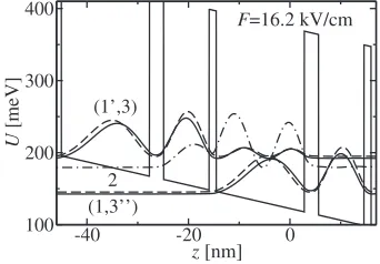
As a prototypical system, we consider a QCL design which comprises a three-level scheme, and employs LO-phonon depopulation of the lower laser level to the ground state. No injector region is present and efficient injection into the upper laser level is enabled by its alignment with the ground level of the preceding period. The QCL period
con-sists of two QWs 共see Fig. 1兲, one of which confines the
ground and lower laser levels, whose energy difference is set
to be approximately one LO phonon energy共36.9 meV兲. The
upper laser level is localized in the other well. This structure was chosen to be examined, instead of existing QCLs al-ready investigated in the presence of a magnetic field, due to its simplicity, and the dominant influence of the electron-LO phonon interaction on the electron population dynamics, as will be explained in what follows.
The conduction band profile and electronic structure of the QCL in zero magnetic field and an electric field of
16.2 kV/ cm, are given in Fig.1. One QCL period includes a
2.8 nm Al0.3Ga0.7As barrier, followed by a 9 nm GaAs well,
a 1.4 nm Al0.3Ga0.7As barrier, and a 17.4 nm GaAs well.
States 1, 2, and 3 represent the ground, lower laser, and
upper laser levels, respectively, and states 1
⬘
and 3⬙
representthe ground level of the preceding period and the upper laser level of the following period. The doping density was chosen
-40 -20 0
z[nm] 100
200 300 400
U
[meV]
F=16.2 kV/cm
[image:7.612.351.522.521.640.2](1,3’’) 2 (1’,3)
to be 1011cm−2, in order to achieve relatively high gain in the THz range, while still having a small influence on the effective conduction band potential and making electron-electron processes less relevant. The temperature was set to 4 K, since QCLs in a magnetic field are usually operated at low temperatures. The transition energy between the upper and lower laser levels is 15.2 meV, and the energy difference between the ground state and the upper laser level of the following period is 2.6 meV.
Relatively strong electron-electron scattering occurs be-tween the ground state and the upper laser level of the next period, due to a large overlap and small energy difference. However, the semiclassical calculation performed for a simi-lar structure showed that the electron-LO phonon scattering rates from the lower laser level to these levels, also relevant for the distribution of electrons between them, are
consider-ably larger.42 Electron-electron processes between other
states are less important, due to the large energy spacing of significantly populated LLs. Consequently, we expect that the population dynamics are not significantly influenced by electron-electron scattering. We make an assumption that the same accounts for the polarization dynamics and as is usual
with quantum-mechanical models of transport in QCLs11–13
we neglect electron-electron scattering hereafter.
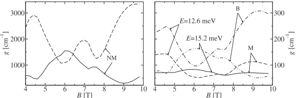
A. Electron populations
The populations of all LLs associated with the ground state and the upper and lower laser levels, calculated using the non-Markovian, Markovian, and Boltzmann model of electron transport, as functions of magnetic field, are shown
in Fig.2. In the calculation, we used the values of the
damp-ing parameter ofប␥= 1 meV andប␥= 2 meV. Regardless of
the model used, the dependencies of the populations on the magnetic field are generally similar. For some values of the
magnetic field共4.6 T, 9.2 T兲, the energy difference between
some LLs stemming from the upper laser level and the ground state becomes equal to one LO phonon energy, thus the electron-LO phonon interaction between them increases considerably. Consequently, the population of all LLs stem-ming from the upper laser level decreases reaching its mini-mum, while the opposite happens to the population of the
LLs stemming from the ground state. Conversely, for
inter-mediate magnetic fields共6.2 T兲, the population of the upper
laser level is increased, while the ground state is depopu-lated. The population of the lower laser level practically does not change with magnetic field.
The populations obtained from the Markovian and Boltz-mann description do not differ much, except in the range of
magnetic fields between 6.2 T and 8 T, see Fig. 2. In the
fully nondiagonal Markovian共and non-Markovian兲approach
employed here, the coupling between populations and polar-izations is accounted for, which results in the presence of phase coherence in the stationary state. In other words, dur-ing the time evolution of the system, scatterdur-ing processes from populations to polarizations create an amount of polar-ization in steady-state conditions. These and reverse
pro-cesses 共dephasing from polarizations to populations兲 may
have an observable impact on electron populations. More pronounced differences between the Markovian and Boltz-mann populations, for magnetic fields between 6.2 T and 8 T, indicate a stronger interplay between populations and polarizations in the Markovian description and, hence, larger
values of polarizations. Indeed, Figs.3 and4 show that the
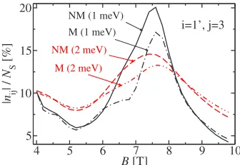
polarizations between all LLs stemming from any two laser states are increased for these magnetic fields.
4 5 6 7 8 9 10
B[T]
0 20 40 60 80
ni
/
NS
[%] i=1i=2
i=3
NM M
B
4 5 6 7 8 9 10
B[T]
0 20 40 60 80
ni
/
NS
[%]
i=1 i=2 i=3
M
[image:8.612.150.466.57.169.2]NM B
FIG. 2. 共Color online兲The electron population over QCL states共all Landau levels兲vs magnetic field. States 1, 2, and 3 represent the ground state, the lower laser level, and the upper laser level, respectively.NSis the total sheet density of electrons per period. Solid, dashed,
and dashed-double-dotted lines represent non-Markovian共NM兲, Markovian共M兲, and Boltzmann共B兲 results, respectively. Left-hand side, ប␥= 1 meV. Right-hand side,ប␥= 2 meV.
4 5 6 7 8 9 10
B[T]
5 10 15 20
|
nij
|/
NS
[%
]
i=1’, j=3
NM (1 meV)
M (1 meV)
NM (2 meV) M (2 meV)
FIG. 3. 共Color online兲 The electron polarization between the ground state of the preceding period and the upper laser level共all Landau levels兲 vs magnetic field. NS is the total sheet density of
[image:8.612.352.520.543.659.2]The Markovian and Boltzmann calculations for different
values of the damping parameter␥showed that the LL
popu-lations are very similar to the corresponding quantum-kinetic
results, see Fig. 2. Nevertheless, this does not mean that
there is one-to-one correspondence between these electron transport models. The non-Markovian description accounts for the memory of scattering and dephasing processes, which corresponds to a quantum-mechanical energy-time uncer-tainty. In comparison, the Markovian or Boltzmann dynam-ics take into account only energy-conserving processes, here, however, relaxed by the assumption that all LLs are broad-ened. This may lead to different values of polarizations, gain, and current although the populations are quite similar.
B. Electron polarizations
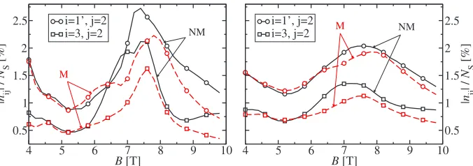
Figures 3 and 4 show the most prominent polarizations
between all LLs associated with pairs of laser states,
ob-tained from the Markovian and non-Markovian models共ប␥
= 1 meV andប␥= 2 meV兲, as they depend on the magnetic
field. In all cases, the polarization between the ground state
and the upper laser level of the next period, shown in Fig.3,
is considerable 共⬃10%兲, due to the fact that these levels
actually constitute a doublet state. Although their overlap does not change with magnetic field, their polarization does, since the LL electronic structure and all scattering and/or
dephasing processes change as well. The polarizations be-tween the upper laser level or the ground state of the previ-ous period and the lower laser level are an order of
magni-tude smaller 共⬃1 %兲, see Fig. 4. This rapidly decreasing
trend continues for the polarizations between other pairs of states, due to strong electron-LO phonon dephasing.
Generally, nondiagonal contribution curves in each Mar-kovian case are offset to smaller values compared to the corresponding non-Markovian ones. This is caused by smaller scattering rates from populations to polarizations in the Markovian case, since they do not include the memory of the interaction. The coherences in the Markovian case for
ប␥= 1 meV have larger peaks than for ប␥= 2 meV, while
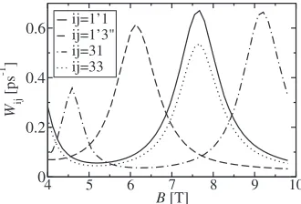
away from the peak, their values become smaller. The effect of smaller broadening is that the scattering rates responsible for the formation of polarizations have larger peak and lower valley values. The same conclusion applies to the non-Markovian results. To illustrate this, the most influential scat-tering rates from populations to the polarization between the states of the doublet in the Markovian case versus magnetic
field are shown in Fig.5. The average scattering rate from
the polarizations between LLs originating from statemi1and
mi
2 into the polarizations between LLs originating from
statesmi4andmi3may be defined in the Markovian approach
according to
4 5 6 7 8 9 10
B[T] 0.5
1 1.5 2 2.5
|
nij
|/
NS
[%]
i=1’, j=2
i=3, j=2 NM
M
4 5 6 7 8 9 10
B[T]
0.5 1 1.5 2 2.5
|
n ij
|/
N S
[%]
i=1’, j=2
[image:9.612.137.475.58.177.2]i=3, j=2 M NM
FIG. 4.共Color online兲The electron polarization between the lower laser level and other QCL states共all Landau levels兲vs magnetic field. States 1⬘, 2, and 3 represent the ground state of the preceding period, the lower laser level, and the upper laser level, respectively.NSis the total sheet density of electrons per period. Solid and dashed lines represent non-Markovian共NM兲and Markovian共M兲results, respectively. Left-hand side,ប␥= 1 meV. Right-hand side,ប␥= 2 meV.
4 5 6 7 8 9 10
B[T]
1 1.5 2 2.5
|
W
2213"
|
[ps
-1 ]
1 meV 2 meV
4 5 6 7 8 9 10
B[T]
0.1 0.2 0.3
|
Wii1
3
"
|
[ps
-1 ]
i=1’ i=3
Wm
i1mi2mi3mi4
a
=
兺
mi 5
兺
ji 1−ji5
n兩mi
1,ji1典兩mi5,ji5典 ⌫兩m
i2,ji2典,兩mi3,ji3典,兩mi4,ji4典,兩mi5,ji5典
out 共␦兩mi4,ji4典,兩mi3,ji3典
−␣Bn兩m
i4,ji4典兩mi3,ji3典兲
兺
mi 5
兺
ji 1,ji5
n兩m
i1,ji1典,兩mi5,ji5典
+
兺
mi 5
兺
ji 1−ji5
n兩mi
5,ji5典兩mi2,ji2典 ⌫兩m
i1,ji1典,兩mi4,ji4典,兩mi3,ji3典,兩mi5,ji5典
out* 共␦兩mi4,ji4典,兩mi3,ji3典
−␣Bn兩mi
4,ji4典兩mi3,ji3典兲
兺
mi 5
兺
ji 1,ji5
n兩mi
5,ji5典,兩mi2,ji2典
. 共33兲
Under the condition thatmi
1=mi2, Eq.共33兲gives the average
scattering rate from LLs associated with state mi1 into the
polarizations between LLs associated with statesmi4andmi3.
Also, the conditionmi1=mi2 andmi3=mi4 gives the average
scattering rate from LLs stemming from state mi1 into LLs
stemming from statemi
3, which is equivalent to the
Boltz-mann scattering rate.
C. Optical gain
In addition to direct transitions of electrons between two
energy states due to emission or absorption of photons 关the
first equation in Eq.共29兲兴, the non-Markovian approach also
accounts for transitions between these states involving
emis-sion or absorption of both photons and LO phonons关see the
denominator in the second equation in Eq.共29兲兴. Since the
latter include an additional influence of LO phonons, it is reasonable to expect that the linewidth of LO phonon-assisted optical transitions is wider in comparison to the one
of direct optical transitions. Indeed, for photon energiesប
which correspond to resonant LO phonon-assisted optical transitions, the gain and/or absorption linewidth is of the
order of 2ប␥ 关see the second equation in Eq. 共29兲兴. On the
other hand, when discussing resonant direct optical transi-tions, we should note that their dynamics are coupled with the dynamics of LO phonon-assisted transitions. Formally, the latter may be interpreted as some kind of scattering pro-cesses, which do not yield energy conservation, but include
an additional ប contribution.41 Therefore, the gain
line-width of direct transitions is determined by these “scattering processes,” whose intensity is strongly influenced by the en-ergy spectra of the system. If resonant LO phonon-assisted transitions do not occur for the same photon energies as di-rect ones, all “scattering rates” are significantly smaller than in the resonant case, and so is the linewidth. In the
Markov-ian description, only direct optical transitions are taken into
account关see Eq.共30兲兴, whose linewidth is determined by the
energy conserving scattering processes, which are strongly dependent on the inter-LL separation. In the Boltzmann ap-proach, the broadening due to the interaction of electrons with light is taken to be equal to the broadening due to the interaction of electrons with LO phonons, consequently, the
linewidth of direct optical transitions is given with 2ប␥.
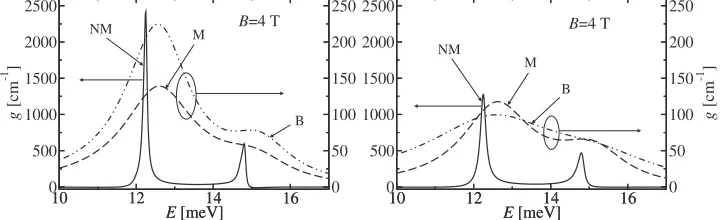
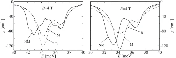
The gain spectra for a magnetic field of 4 T in the energy range close to the laser transition energies and one LO
pho-non energy, are shown in Figs. 6 and 7, respectively. The
gain coefficient was calculated for the non-Markovian,
Mar-kovian, and Boltzmann dynamics 共ប␥= 1 meV and ប␥
= 2 meV兲. In the case of resonant direct optical transitions
between either the upper laser level or the ground state of the
previous period and the lower laser level 共ប⬇E¯3−E¯2 or
ប⬇E¯1⬘−E¯2, respectively兲, there is no additional
contribu-tion of resonant LO phonon-assisted optical transicontribu-tions for the QCL considered. In contrast, for photon energies close to one LO phonon energy, such contributions do appear, and are related to absorption of photons followed by emission of phonons with no electron transitions involved or with
elec-tron transitions between energetically close states共the upper
laser level and the ground state of the previous period兲.
Con-sequently, the gain linewidth for the energies corresponding to the laser transitions is considerably smaller than for the
energies around one LO phonon energy, compare Figs.6and
7. However, in a real QCL device, it is likely that the
inter-action of electrons with impurities, interface defects, and other electrons, as well as imperfect periodicity, will broaden the LLs making the gain linewidth for laser transition ener-gies not as narrow as the non-Markovian model predicts.
In the Markovian description, since the LO phonon reso-nances between the lower laser level and either the ground state or the upper laser level of the next period are present in
10 12 14 16
E[meV]
0 500 1000 1500 2000 2500
g
[cm
-1 ]
10 12 14 16
E[meV]
0 50 100 150 200 250 B=4 T
NM M
B
10 12 14 16
E[meV]
0 500 1000 1500 2000 2500
10 12 14 16
E[meV]
0 50 100 150 200 250
g
[cm
-1 ]
B=4 T
NM
M
[image:10.612.51.411.624.734.2]B
FIG. 6. Optical gain vs energy for a magnetic field of 4 T. The energy range is in the vicinity of the laser transition energies. Solid, dashed, and dashed-double-dotted
lines represent non-Markovian
共NM兲, Markovian共M兲, and Boltz-mann 共B兲 results, respectively.
Left-hand side, ប␥= 1 meV.
the energy spectra, the corresponding resonant scattering terms lead to large linewidths of gain features throughout the
frequency range of interest共considerably larger than the
non-Markovian linewidth for the laser transition energies and comparable to the non-Markovian linewidth for energies
close to one LO phonon energy兲. We should note that, if
there were no such LO phonon resonances in the system, the gain linewidth in the Markovian description would be smaller. As a consequence, we observe a significant differ-ence between the Markovian and non-Markovian gain line-width for the laser transition energies. A similar result for direct optical transitions at low temperatures in quantum wells without magnetic field has also been reported in Ref.
18.
In the Markovian limit, energy renormalizations, describ-ing the polaron corrections to the band structure, are ignored. However, the polaron shift is always included in the quantum-kinetic treatment. It is more prominent for the
en-ergy transitions close to one LO phonon enen-ergy共⬃1 meV兲,
but it is also present for the laser transition energies
共⬃0.4 meV兲.
Figure8illustrates the gain profile for a magnetic field of
6 T in the energy range around the laser transition energies and one LO phonon energy, calculated from the
non-Markovian model forប␥= 1 meV andប␥= 2 meV.
Compari-son of the non-Markovian gain spectra for different values of
the damping parameter共see also Figs.6 and7兲reveals
pro-nounced differences between both the gain linewidth and peak values. Sensitivity of the results to the values of the phenomenological parameter confirms the need for a self-consistent incorporation of higher-order correlations in the quantum-kinetic model, which would require a significant
increase in computational time. Moreover, for a magnetic field of 6 T, apart from the two expected peaks associated with the transitions from the lower laser level to the ground state or the upper laser level of the subsequent period, which are in the vicinity of one LO phonon energy, an extra peak at
ប= 34.3 meV appears for ប␥= 1 meV, in comparison to
ប␥= 2 meV, see Fig. 8. This is due to the fact that, for the
electronic structure of the QCL considered, peaks due to resonant LO phonon-assisted optical transitions may also
emerge in that energy range. Careful inspection of Eq.共29兲
reveals the presence of resonances at the energies of ប
⬇±共E兩3⬙j典−E兩1,j典兲+បLO= ± 2.6 meV+បLO, as discussed
earlier. At first, it may appear that one of these resonances, related to the transition between the ground state and the upper laser level of the subsequent period, is manifested via
that additional peak in the gain and/or absorption spectra共a
so-called polaron satellite兲.18However, this is not entirely the
case here. Due to a nontrivial interplay between these reso-nant LO phonon-assisted terms, and resoreso-nant direct optical transitions from the lower laser level to the ground state or the upper laser level of the following period which occur at
similar energies, ⌬n兩1,j典兩2,j典共兲 or ⌬n兩3⬙,j典兩2,j典共兲 constitute a
much larger fraction of the total gain for energies close to
បLO than ⌬n兩3⬙,j典兩1,j典共兲. Here, the peak at ប= 34.3 meV
for B= 6 T and ប␥= 1 meV is actually related to the
transi-tion between the lower laser level and the upper laser level of
the next period 关the calculation showed that ⌬n兩1,j典兩2,j典共兲
⬍ ⌬n兩3⬙,j典兩2,j典共兲兴, as well as the peak atប= 32.7 meV which
is also present for ប␥= 2 meV, while the peak at ប
= 36.8 meV is associated with the transition between the lower laser level and the ground state. In fact, the previous analysis of the terms which are resonant for the energies in
30 32 34 36 38 40
E[meV]
-120 -80 -40 0
g
[cm
-1 ]
B=4 T
NM
M
B
30 32 34 36 38 40
E[meV]
-120 -80 -40 0
g
[cm
-1 ]
B=4 T
[image:11.612.157.459.58.159.2]NM M B
FIG. 7. Optical gain vs energy for a magnetic field of 4 T. The energy range is in the vicinity of one longitudinal optical phonon energy. Solid, dashed, and dashed-double-dotted lines represent non-Markovian共NM兲, Markovian共M兲, and Boltzmann共B兲 results, respectively. Left-hand side,ប␥= 1 meV. Right-hand side,ប␥= 2 meV.
10 12 14 16
E[meV]
0 500 1000 1500
g
[cm
-1 ]
B=6 T
NM (2 meV)
NM (1 meV)
30 32 34 36 38 40
E[meV]
-250 -200 -150 -100 -50 0
g
[cm
-1 ]
B=6 T
[image:11.612.156.457.594.694.2]NM (1 meV) NM (2 meV)