The Development and Application
of Real-Time Protein Interaction
Technology
Thesis submitted in accordance with the
requirements of the University of Liverpool for the
degree of Doctor in Philosophy by
Nicholas Aled Jones
Acknowledgements
Thanks go to both Dr. Daimark Bennett and Prof. Mike White for all their help and encouragement over the course of this PhD.
Thank you to everyone in the Bennett Lab for all the help, to Anita, Nick, Louise, Neville, Lauren, Vincent, Peter, and especially to Eleanor for all those Drosophila skills I put to such good use and keeping me company in the fly lab at ridiculous hours of the night. Thanks must of course also go to Chris L for generally keeping me sane and sharing in the joy of constant failure. Thanks to Jean for letting me annex so much lab space in lab G and not making too much of my messy desk!
Declaration
This thesis is the result of my own work unless otherwise stated, and is based upon results from experimental and theoretical work performed as a PhD student between Opctober 2008 and September 2012 in the department of biological sciences within the University of Liverpool and in the University of Manchester.
Neither this thesis nor any part of it has been submitted in support of an application for another degree of qualification at this or any other University of other institute of learning.
Nicholas Jones
Abstract
Protein interactions are a fundamental part of cellular processes, and represent a key target in the understanding of cell behaviour, communication and function. These interactions are dynamic in nature, and change over time. Furthermore, interactions can be dependent on co-localisation in cellular compartments. Both of these characteristics can be obscured through observation by bulk molecular cell assays such as co-immunoprecipitation (co-IP) and can obscure the intricacies of single cell dynamics.
The development of tools and new methodologies to observe single cell protein interaction dynamics are key to understanding the underlying mechanisms that direct cell fate. Systems biology aims to incorporate into predictive models of the whole system. In this way, the development of quantitative experimental tools is a key component of systems biology. Förster Resonance Energy Transfer is a widely used technique in the field of protein-protein interaction studies. Dependent on the non-radiative transfer of energy from a fluorescent molecule of higher excitation energy to a fluorescent molecule of lower excitation energy with sufficiently overlapping spectra, the process occurs across a 1-10nm (100Å) range. As a result, FRET interactions between fluorophores attached to biologically functional proteins are a strong indication of protein interaction.
The photoswitchable protein Dronpa offers a unique opportunity to develop a real-time live cell variant of this technique. Through the modulation of Dronpa fluorescence, repeated donor quenching can be observed, allowing quantification of FRET interactions between fluorophores without spillover. This is achieved sequentially through the optimisation of Dronpa imaging parameters for live cell imaging, followed by the identification and testing of candidate FRET partners using an optimised imaging protocol. Direct fusions were used to qualify potential FRET responses between tested pairs of fluorophores. FRET responses using positive control constructs were rigorously tested and quantified to ensure repeatable and consistent reporting of FRET. The spectral properties of Dronpa and chosen FRET partners were also rigorously tested to ensure FRET could be accurately measured through sensitised emission.
Contents
Abstract ... i
Contents ... ii
List of Figures and Tables ... vi
Commonly Used Abbreviations ... x
Chapter 1:
Introduction
...1
1.1- Introduction I - The Importance of Protein Interactions ... 2
1.1.1 The Protein ... 2
1.1.2 Observing Protein Interactions ... 3
1.2 Introduction II - The Imaging Toolbox ... 5
1.2.1 Microscopy and Confocal Microscopy ... 5
1.2.2 Fluorescent Proteins ... 6
1.2.3 Exotic Fluorescent Proteins ... 11
1.2.3.1 Dronpa ... 12
1.2.4 Fluorescence Resonance Energy Transfer ... 14
1.2.4.1 Crosstalk Correction and Sensitised Emission ... 18
1.2.4.2 Acceptor photobleaching ... 19
1.2.4.3 Artefacts and Issues ... 20
1.2.5 Fluorescence Correlation Spectroscopy ... 21
1.3 Introduction - III The NF-κB Signalling Pathway ... 24
1.3.1 NF-κB Overview ... 24
1.3.2 NF-κB Family Members ... 24
1.3.3 Multicellular Model Systems ... 31
1.4 Project Aims ... 32
Chapter 2:
Materials and Methods
...34
2.1 Materials ... 35
2.1.1 Reagents ... 35
2.1.2 Expression Vectors... 35
2.2 Molecular Biology ... 35
2.2.1 Transformation of Chemically Competent E. coli Cells ... 35
2.2.2 DNA Purification ... 36
2.2.2.2 Large Scale DNA Extraction (Maxi-prep) ... 36
2.2.3 DNA Quantification ... 37
2.2.4 Restriction Endonuclease Digests ... 37
2.2.5 Gel Electrophoresis ... 37
2.2.6 PCR and introducing Cut Sites ... 38
2.2.7 Site Directed Mutagenesis... 39
2.2.8 5’-Phosphate removal... 40
2.2.9 Ligation and Transformations ... 40
2.2.10 Directional TOPO® Cloning ... 41
2.2.11 Generating mRNA and cDNA from Genomic DNA ... 41
2.2.12 DNA synthesis ... 41
2.2.13 Gateway system and recombination ... 42
2.2.14 DNA Sequencing ... 42
2.3 Cell culture ... 43
2.3.1 Subculturing cells ... 43
2.3.2 Transient Transfection and Imaging ... 43
2.3.3 TNFα Treatment ... 43
2.3.4 Drosophila S2R+ Cell culture ... 44
2.3.5 S2R+ Transfection ... 44
2.3.6 Stimulation with Latrunculin ... 44
2.4 Western Blotting ... 45
2.4.1 Preparation of Protein Samples ... 45
2.4.2 Preparation of SDS-PAGE Gels... 45
2.4.3 Protein Separation by SDS-PAGE ... 45
2.4.4 Transfer of Electrophoresed Proteins to Nitrocellulose ... 46
2.4.5 Probing Membrane ... 46
2.5 Imaging Techniques ... 47
2.5.1 Live-Cell Imaging ... 47
2.5.2 FRET: Optimised Illumination Strategy ... 48
2.5.3 FCS and FCCS ... 49
Chapter 3:
Tools and Optimisation
...50
3.1 Introduction ... 51
3.3 Dronpa Photoswitching Optimisation ... 52
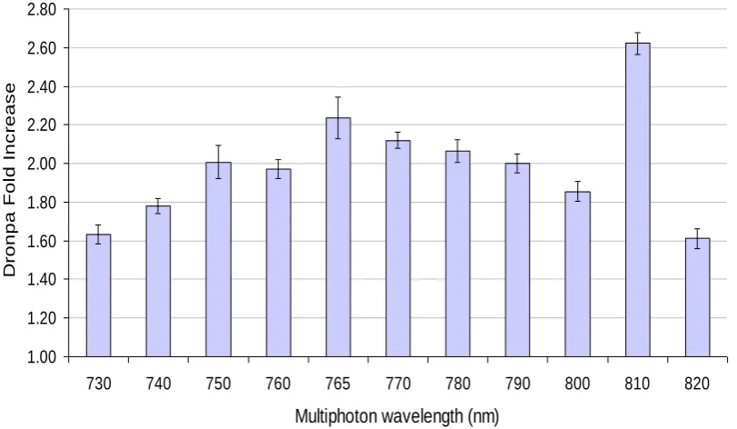
3.3.1 Multiphoton Excitation ... 53
3.3.2 Switching Dronpa with 405nm Excitation ... 55
3.3.3 Effect of extracellular pH on Dronpa Switching Efficiency. ... 56
3.3.4 Dronpa Fusion Characteristics ... 57
3.4 FRET Partners ... 59
3.4.1 Cyan Partners ... 61
3.4.2 Enhanced Cyan Fluorescent Protein ... 62
3.4.3 mTeal Fluorescent Protein ... 63
3.4.4 AmCyan ... 64
3.4.5 Red Partners ... 66
3.4.6 DsRedExpress ... 67
3.4.7 mStrawberry ... 68
3.4.8 tdTomato & mCherry ... 69
3.5 Positive Controls and Construct Creation ... 70
3.5.1 AmCyan Positive Control ... 71
3.5.2 Strawberry Positive Control ... 74
3.6 Reverse Dronpa Switching Strategy ... 75
3.7 Conclusion ... 76
Chapter 4:
Qualifying and Quantifying FRET
...
77
4.1 Rationale for Quantification ... 78
4.2 Zeiss Spectral Deconvolution ... 78
4.3 Manual Linear Unmixing ... 80
4.3.1 Unmixing AmCyan ... 80
4.3.2 Unmixing mStrawberry ... 83
4.4 Donor Relationship with Sensitised Emission ... 85
4.4.1 Donor and Acceptor Saturation ... 87
4.5 Quantification ... 88
4.5.1 Normalisation of Populations ... 91
4.5.2 Calculating FRET Efficiency ... 92
4.6 Conclusion ... 94
Chapter 5:
FRET in the NF-κB System
...96
5.2 The Characterisation of p105 ... 98
5.3 FRET in p105 ... 101
5.3.1 Intermolecular p105 interactions... 103
5.3.2 Changes in p105 over time ... 106
5.4 Dynamics of p105 using FCCS ... 117
5.4.1 Effect of p65 on full length p105 ... 121
5.5 Intermolecular p105 Interactions ... 122
5.5.1 p65/p50 ... 124
5.5.2 Interaction of p105/p65 using FCS ... 126
5.6 Discussion ... 128
5.6.1 The Dynamics of NF-κB1 ... 128
Chapter 6:
General Discussion
...130
6.1 Summary of main discoveries in thesis ... 131
6.2 Relationship of real-time FRET assay to protein interaction assays .. 132
6.2.1 Biochemical Assays ... 132
6.2.2 Biophysical Assays ... 134
6.2.3 Protein-Fragment Complementation Assays ... 135
6.2.4 Fluorescence Fluctuation Assays ... 136
6.2.5 Discussion of Techniques in Context ... 137
6.3 Remaining issues in live cell FRET ... 138
6.3.1 Improvements to the Assay ... 139
6.4 Biological insights into p105 ... 140
6.5 Potential future work: 3 way FRET, and applications in model species eg Drosophila. ... 141
6.6 Future of live cell imaging and systems biology ... 143
List of Figures and Tables
Figures
Figure 1-1 Abbe’s Equation estimating diffraction limit of a microscope. .. 5
Figure 1-2 Spectral overlap of ECFP and EYFP. ... 14
Figure 1-3 Diagram demonstrating the basic principle of FRET. ... 15
Figure 1-4 Data illustrating acceptor photobleaching... 19
Figure 1-5 Diagrammatic representation of FCS and FCCS. ... 23
Figure 1-6 Diagram depicting NF-κB proteins ... 26
Figure 1-7 Schematic of NF-κB signalling. ... 30
Figure 3-1 Illumination to activate and inactivate Dronpa fluorescence. ... 52
Figure 3-2 Effect of multiphoton wavelength on Dronpa switching. ... 54
Figure 3-3 Effect of the number of iterations of illumination at 810nm on Dronpa switching. ... 55
Figure 3-4 Effect of 405nm laser power on Dronpa switching. ... 56
Figure 3-5 Effect of pH condition on Dronpa Switching. ... 57
Figure 3-6 Variability of Dronpa fluorescence when expressed in various fusion proteins. ... 58
Figure 3-7 Efficiency of Dronpa switching in different fusion proteins. ... 59
Figure 3-8 Excitation and emission spectra of Dronpa. ... 60
Figure 3-9 The spectral overlap of Cyan family fluorescent proteins with Dronpa. ... 61
Figure 3-10 ECFP fluorescence and susceptibility to bleaching when subjected to the switching protocol for Dronpa. ... 62
Figure 3-11 Evaluation of mTeal fluorescent protein. ... 63
Figure 3-12 Effect of pulsing with 405nm illumination on the fluorescence from AmCyan in single cells. ... 64
Figure 3-13 AmCyan can show a small increase in fluorescence following pulsing with 405nm excitation ... 65
Figure 3-14 Emission spectrum of Dronpa (dashed line) overlaid with the absorbtion spectra of the red fluorescent proteins. ... 66
Figure 3-16 Characterisation of the properties of mStrawberry as a potential
acceptor for Dronpa. ... 68
Figure 3-17 Properties of mCherry and tdTomato... 69
Figure 3-18 Imaging of control fluorescent proteins with AmCyan as acceptor and Dronpa as donor in two orientations. ... 72
Figure 3-19 FRET between AmCyan and Dronpa in the control fusion proteins. ... 73
Figure 3-20 FRET between Dronpa and mStrawberry in positive control. .. 74
Figure 3-21 Reverse Dronpa switching strategy results in less efficient change in Dronpa fluorescence. ... 75
Figure 4-1 Problems encountered using Zeiss AIM linear unmixing algorithms... 79
Figure 4-2 Relative fluorescence spillover in single cells ... 80
Figure 4-3 An example of spillover correction with Dronpa acceptor ... 81
Figure 4-4 Spillover in a cell population with Dronpa acceptor. ... 82
Figure 4-5 Spillover correction of the Signal from a positive control for FRET. ... 83
Figure 4-6 Spillover between Dronpa and mStrawberry. ... 84
Figure 4-7 Spillover correction of Dronpa mStrawberry FRET ... 84
Figure 4-8 The relationship between sensitised emission (FC) and donor quenching ... 85
Figure 4-9 The relationship of ‘G’ with Dronpa protonation state. ... 86
Figure 4-10 The relationship between FC and acceptor:donor ratio. ... 87
Figure 4-11 Example data from cells expressing different fusion pairs. ... 89
Figure 4-12 A comparison of outputted FRET images from Image J Plug in Fret Analyser. ... 90
Figure 4-13 A comparison of Dronpa switching in cell populations expressing positive and negative FRET control constructs ... 91
Figure 5-1 Western blot of endogenous N-terminal p105 levels ... 98
Figure 5-2 Western blot of endogenous and transiently transfected N-terminal p105 ... 99
Figure 5-4 A comparison of the Intracellular FRET response from different transfections. ... 102 Figure 5-5. A comparison of the FRET efficiency between and within p105
proteins. ... 103 Figure 5-6 Change in donor fluorescence following acceptor
photobleaching ... 105 Figure 5-7 Changes in p105 fluorescent signals in a single cell over time.
... 106 Figure 5-8 The Changes in fluorescence signal in Single cells over time. 107 Figure 5-9 Changes in FRET over time. ... 109 Figure 5-10 Time-dependent changes in Dronpa fluorescence localisation.
... 110 Figure 5-11. Changing FRET efficiency of an example cell over time. ... 111 Figure 5-12 Comparison of FRET efficiency between nuclear and
cytoplasmic compartments ... 113 Figure 5-13 Normalised change in quenching efficiency in single cells .... 114 Figure 5-14 Changing FRET efficiency of a cell over time. ... 116 Figure 5-15. Cross-correlation and autocorrelation curves for SK-N-AS cells
expressing protein from pG-DsRed-p105-EGFP ... 118 Figure 5-16 - Cross-correlation and autocorrelation curves for SK-N-AS
transfected with pG-CMV-DsRed-p105-EGFP ... 119 Figure 5-17. Quantification of DsRed-p105-EGFP fluorescence expressed in
SK-N-AS cells... 120 Figure 5-18. Effect of p65 on p105 FRET efficiency. ... 121 Figure 5-19 Array of intermolecular FRET interactions with p105. ... 122 Figure 5-20 FRET in Cells expressing pG-CMV-Dronpa-p65 pG-CMV-p50-AmCyan. ... 123 Figure 5-21 Changes in intermolecular FRET between
pG-CMV-p65-AmCyan and pG-CMV-Dronpa-p105 in a single cell treated with TNFα. ... 125 Figure 5-22 Cross-correlation and autocorrelation curves for p65 and N and
Tables
Table 1-1 Sample list of Fluorescent Protein properties ... 8
Table 1-2 Example Optical Highlighter fluorescent proteins. ... 12
Table 1-3 A list of abbreviations for FRET filter combinations. ... 18
Table 2-1 Agarose Gel Percentages for DNA Fragment Separation ... 38
Table 2-2 Time lapse imaging parameters ... 48
Table 3-1 List of control constructs... 71
Commonly Used Abbreviations
aa Amino Acid
β-ME 2-Mercaptoethanol
AFP Aequorea Derived Fluorescent Protein AOTF Acousto-optical tuneable filter
APD Avalanche Photo Diode ATP Adenosine triphosphate
AU Arbitrary Units
att Attachment Site
BSA Bovine Serum Albumin CCD Charged Coupled Device cDNA Complementary DNA CMV Cytomegalovirus
Co-IP Co-Immuno Precipitation CSS Charcoal-Stripped Serum Cyto Cytoplasm
DD Death Domain
DMEM Dulbecco’s Modified Eagle’s Medium DNA Deoxyribonucleic Acid
dNTP Deoxynucleotide Triphosphate
dsRed Red Fluorescent Protein (from Discosoma) dsRed-XP dsRed-Express
ECFP Enhanced Cyan Fluorescent Protein EGFP Enhanced Green Fluorescent Protein EYFP Enhanced Yellow Fluorescent Protein FC Sensitised emission
FCS Foetal Calf Serum
FCS Fluorescence Correlation Spectroscopy FCCS Fluorescence Cross-Correlation Spectroscopy FRET Fluorescence Resonance Energy Transfer galvo Scanning Galvanometer Mirror
GRR Glycine-Rich Region
IKK IκB Kinase
IL Interleukin
It. Iteration
IκB Inhibitor-κB
LN2 Liquid Nitrogen
LPS Lipopolysaccharide
LSM Laser Scanning Microscope MCS Multiple Cloning Site
mRNA Messenger RNA
mRaspberry Monomeric Raspberry Fluorescent Protein mRFP Monomeric Red Fluorescent Protein
mStrawberry Monomeric Strawberry Fluorescent Protein mTFP Monomeric Teal Fluorescent Protein
NA Numerical Aperture
NEMO NF-κB Essential Modulator NES Nuclear Export Signal NF-κB Nuclear Factor-κB NIK NF-κB-Inducing Kinase NLS Nuclear Localization Signal
Nuc Nucleus
PBS Phosphate-Buffered Saline PCR Polymerase Chain Reaction
PEST Proline, Glutamic Acid, Serine, Threonine Rich Region PMT Photo Multiplier Tube
PR Progesterone Receptor RHD Rel-Homology Domain RIP Receptor Interacting Protein RNA Ribonucleic Acid
ROI Region of Interest
RTKs Receptor Tyrosine Kinases
SD Standard Deviation
TAD Transactivation Domain
TAE Tris-Acetate/EDTA Electrophoresis Buffer TBS Tris-Buffered Saline
TBS-T TBS with Tween-20)
TEMED N,N,N′,N′-Tetramethylethylenediamine TNFR TNF Receptor
TNFα Tumour Necrosis Factor
TRADD TNF Receptor-Associated Death Domain Protein TRAF TNF Receptor Associated Protein
Tris Tris(hydroxymethyl)methylamine UV Ultra violet light
1.1- Introduction I – The Importance of Protein Interactions
1.1.1 The Protein
Proteins are functional products of genes encoded in genetic DNA, the fundamental building blocks of life, and key to cell communication, function and survival. In collaboration, proteins have the power to direct cell fate through apoptosis and proliferation and migration or can function benignly as structural sub units such as collagen.
Proteins control cell processes and behaviour at almost every level, from the endocrine and paracrine inter-communication of cells through excretion of proteins into the inter cellular matrix to the control of early and late gene expression through time-dependent or conditional nuclear translocation of transcription factors (Nelson, Ihekwaba et al. 2004; Bancos, Natt et al. 2012). Some processes like the transduction of intercellular signals following treatment with Tumour Necrosis Factor α (TNFα) result in a signalling cascade involving the phosphorylation and degradation of many transient protein interactions or the movement of cells through the formation of actin rich protrusions known as lamellapodia facilitating cell migration, proliferation and growth. Such processes are key to cell survival and multicellular interaction (Tartaglia and Goeddel 1992; Lyulcheva, Taylor et al. 2008).
Protein interactions are often dynamic and can mediate changes in protein activity or subcellular localisation (such as the shuttling of proteins to and from the nucleus (Hayden and Ghosh 2004)). These interactions can be transient (Nooren and Thornton 2003) or long lived (Heessen, Masucci et al. 2005) depending on the nature of the response. Understanding where and when protein interactions occur is of critical importance to understanding the role and regulation of these proteins in cellular processes.
Heterogeneity between individual cells is a well known feature of dynamic cellular processes. This heterogeneity has been suggested to confer a significant advantage in maintaining robustness in overall coordination and stability of cell population responses (Paszek, Ryan et al. 2010).
This gives single cell data particular significance. Molecular methods for observing protein levels and binding partners not only require the denaturing of proteins, the lysing of cells and destruction of intracellular compartmentalisation; they also rely on large populations of cells, giving an indiscriminate global picture of cell response to stimuli. Non-invasive methods of measuring cellular processes in the same cell over time are necessary to gain a deeper understanding of what protein behaviours occur in cell populations. With the capability of measuring protein-protein interactions, protein movement and transcriptional output from single living cells (Rutter, White et al. 1995; Stirland, Seymour et al. 2003; Nelson, Ihekwaba et al. 2004; See, Rajala et al. 2004).
1.1.2 Observing Protein Interactions
There are many methods of observing protein interactions, all with their own advantages and disadvantages. Methods can broadly be separated into two categories; Biochemical assays and biophysical methods.
of observing protein interactions is that the interactions could be occurring in the cell lysate following disruption of the cell structures, so it may not be a true representation of the interactions occurring within an intact cellular compartment. Conversely, intracellular compartmentalisation can affect any number of cellular processes and the ability of a protein to form a complex and its subsequent behaviour.
1.2 Introduction II- The Imaging Toolbox
1.2.1 Microscopy and Confocal Microscopy
Light Microscopy has been in general use in biology for over 300 years. In fact the term cell originates from Robert Hooke and his comparison of cork cells to that of monks’ cells while using a compound microscope (Fara 2009). Over that time, light microscopy has become more refined and complex to the extent that the main limiting factor for obtaining higher resolution through traditional means are the physical properties of light and diffraction in relation to refractive index.
Figure 1-1 Abbe’s Equation estimating diffraction limit of a microscope.
d is the resolvable distance, λ is the wavelength of light, n is the refractive index of the medium being imaged in, and θ is half the angle of the cone of light from specimen plane accepted by the objective.
In his paper of 1873, Abbe reported that the smallest resolvable distance between two points using a conventional microscope cannot be smaller than half the wavelength of the imaging light (Abbe 1873). Abbe concluded that the resolution was limited by diffraction to half the wavelength modified by the refractive index of the medium and the angle of the cone of focused light (Figure 1-1). Based on this equation, it is possible to improve spatial resolution either by increasing the numerical aperture, which is limited by the refractive index the image is observed though, or by using light with a shorter wavelength (e.g. ultraviolet). This, however, risks damage to biological samples through oxidative stress or DNA damage (depending on the wavelength), and is undesirable due to increased light scattering within a tissue. Conversely, longer wavelengths improve tissue penetration at the expense of resolution (Wang, Konig et al. 2010).
epifluoresence microscopy meant for the first time labelling of cellular structures and proteins could be used to study more subtle elements of cell structure and function (Coons, Creech et al. 1941). However, resolution of samples remained an issue.
The solution was conceived through the design and implementation of the confocal microscope (Egger and Petran 1967). Traditional widefield epifluoresence is hindered by out of focus light from the sample and ambient sources. By including a confocal aperture before a detector, out of focus light is removed from the sample (Sheppard and Wilson 1981; White, Amos et al. 1987). The inclusion of the aperture means samples must be raster scanned and build up digitally via photon to electron conversion using Photo Multiplier Tubes (PMT) or various other types of photon detector. This is achieved through movement of the point of illumination by X and Y galvo mirrors (White, Amos et al. 1987). Modern confocal microscopes make use of laser excitation, which is monochromatic, polarised and coherent and has the advantage of converging via the objective, at a single point of excitation in the focal plane of the sample eliminating the need for a pinhole at the light source (van Meer, Stelzer et al. 1987). The combination of confocal microscopy with the discovery of fluorescent proteins and their application as fusion partners in proteins complexes, has become invaluable to studies of single cell and protein behaviour (Chalfie, Tu et al. 1994; Shaner, Patterson et al. 2007).
1.2.2 Fluorescent Proteins
fluorophores has grown exponentially (Shaner, Steinbach et al. 2005; Shaner, Patterson et al. 2007). There is now a wide variety of colours, improved maturation time (Mikkelsen, Sarrocco et al. 2003), improved quantum yield and stability (Shaner, Patterson et al. 2007) and novel behaviours such as photoactivation and photoconvertibility (Chudakov, Verkhusha et al. 2004; Henderson and Remington 2006; Bourgeois and Adam 2012).
Table 1-1 Sample list of Fluorescent Protein properties
obtained from Shaner et. al. (Shaner, Campbell et al. 2004)1(Shaner, Patterson et al. 2007)2
(Padilla-Parra, Auduge et al. 2009)3 *weakly dimerised in high concentrations.
Name Structure
Excitation
Max
(nm)
Emission
Max
(nm)
Relative
Quantum
Yield
Excitation
Coefficient
(M-1cm-1)
Brightness
Red
mRaspberry1 Monomer 598 625 0.15 86,000 12,900
mCherry1 Monomer 587 610 0.22 72,000 15,840
mStrawberry1 Monomer 574 596 0.29 90,000 26,100
mRFP1 Monomer 558 583 0.25 50,000 12,500
DsRedEx Tetramer 563 579 0.90 19,000 17,100
Orange
tdTomato1 Tandem
Dimmer 554 581 0.69 69,000 47,610
Yellow
EYFP2 Monomer* 514 527 0.85 64,000 54,400
Green
EGFP2 Monomer* 484 510 0.70 23,000 16,100
Dronpa4 Monomer 503 518 0.62 57,000 35,340
Cyan
mTFP3 Monomer 462 492 0.85 64,000 54,400
AmCyan2 Tetramer 458 489 0.85 44,000 37,400
ECFP2 Monomer* 439 476 0.40 32,500 13,000
The expression of fusion proteins in live cells, it might be argued, is comparatively less invasive than fixation. Through introducing cDNA for transient expression or permanent integration into cell chromosomes, protein structure and function is usually maintained (Felgner, Gadek et al. 1987). This allows images of the same live cells to be collected over time, and it becomes possible to observe many different cell processes and responses in an individual cell such as responses to specific stimuli, in real time. An example of this can be seen in the NF-κB pathway and with TNFα treatment and the resulting oscillations in p65 nuclear cytoplasmic localisation (Nelson, Ihekwaba et al. 2004).
Two possible artefacts that are important for consideration when expressing fusion protein constructs are over-expression and interference with wild type behaviour. Simply by introducing fusion constructs into cell lines without first inhibiting or removing endogenous protein expression could be considered as over-expression of a protein. Over-expression is more often than not considered the point at which protein level saturates the cell’s machinery. It may be more accurate to describe expression of a fluorescent protein fusion from a viral (eg. CMV) promoter as “out of context” as the protein might be expressed constitutively and not regulated at the transcriptional level by the protein's own promoter.
Achieving a more physiological level of expression is no mean feat. Transient transfection offers no control of over-expression other than selecting cells with the appropriate level (Spector and Goldman 2006). Short of using molecular counting techniques like fluorescence correlation spectroscopy (FCS) or calibration of intensity with known standards, quantification of protein level is difficult.
constructs as the long flanking sequences can act to insulate the gene of interest from site of integration effects (de Wet, Wood et al. 1987).
It is also important to ensure that the label being fused to the target protein has had no effect on wild type protein function or behaviour. Linker sequences or even fluorophore size and termini position might affect protein behaviour. Controls such as Ires vectors (separately expressing protein and FP from a single transcription event by ribosomal skipping of the linking sequence) can be used to ensure cell behaviour remains consistent.
Important qualities of fluorescent proteins include brightness, photostability, oligomerisation, environmental sensitivity and spectral excitation and emission profiles (Shaner, Steinbach et al. 2005). Brightness is a rather arbitrary determinate of an FP’s aptitude, it is determined by its maturation speed and efficiency, extinction coefficient, and quantum yield and effected by filter set efficiency on the system in use for any given spectra. Brightness is best considered alongside photostability, as fluorophores that are overexcited will begin to bleach. In experimental situations, where expression level is of significance this can affect results (Shaner, Steinbach et al. 2005; Shaner, Patterson et al. 2007). The best way of establishing the usefulness of a particular FP under a given set of experimental parameters is to image the freely-expressed fluorophore in the correct live cell context.
Oligomerisation of fluorescent proteins could potentially cause fusion proteins to form complexes through fluorophore interactions. This is of particular importance for molecular counting techniques such as FCS which can use relative molecular brightness as a measure of protein oligomerisation (Chen, Wei et al. 2003). Environmental sensitivity can affect fluorophore folding, either through pH sensitivity, oxygen requirement or temperature-dependent folding. An example of the importance of oxygen sensitive folding is the difference between Aequorea-derived fluorescent proteins and red shifted coral fluorophores. These red fluorophores generate twice the number of H202 molecules than that of AFPs indicating that twice
(Tsien 1998; Gross, Baird et al. 2000). Folding temperature should also be considered when selecting FPs, for example the fluorophore CyPet folds poorly at 37ºC limiting its use for in vivo expression in mammalian model systems (Shaner, Patterson et al. 2007).
Spectral emission and excitation profiles are most important when imaging multiple fluorophores in the same system. While linear unmixing provides the ability to separate emission from overlapping spectra, a more straightforward approach is to choose fluorophores with appropriate spectral separation. ECFP (Figure 1-2) for example has a wide emission spectra, this means it is a poor choice for spectrally separate imaging with other FPs such as EGFP (Patterson, Day et al. 2001).
1.2.3 Exotic Fluorescent Proteins
Table 1-2 Example Optical Highlighter fluorescent proteins.
Photoconvertable, photoswitchable, and photoactivatable fluorescent proteins (Habuchi, Ando et al.
2005)1(Chudakov, Belousov et al. 2003)2(Patterson and Lippincott-Schwartz 2002)3. (Gurskaya,
Verkhusha et al. 2006)4
Photoswitchable fluorophores have the unique possibility of being used as FRET partners which can be modulated. This gives a huge advantage in the ability to repeatedly quantify FRET in-vivo using the principle of acceptor photobleaching (see 1.2.4). Dronpa and Kindling show clear superiority in their ability to be switched repeatedly, and also have the added advantage of being spectrally separate (Table 1-2) suggesting that both could be used simultaneously in vivo.
1.2.3.1 Dronpa
First developed by Ryoko Ando, Hideaki Mizuno, and Atsushi Miyawaki in 2004 (Ando, Mizuno et al. 2004), Dronpa is a robust photoswitchable fluorescent protein which has been demonstrated to be switchable more than 100 times on the single molecule level (Habuchi, Ando et al. 2005). The absorption maximum of Dronpa is at 503nm, and emission spectra peaks at 518nm. While illumination with 488nm causes the fluorophore to fluoresce , it simultaneously converts the fluorophore into a dim state. In this dim state, Dronpa has a different absorption peak of 390nm. Minimal UV excitation at 405nm is required to convert Dronpa back to its bright state, (Ando, Mizuno et al. 2004; Habuchi, Ando et al. 2005).
Name Classification Excitation Max(nm)
Emission
Max(nm)
Activation
wavelength
Quantum
Yield
Extinction
Coefficient
(M-1cm-1)
Dronpa1 Photoswitchable 503nm 518nm 405nm 0.79 17,400
Kindling1 Photoswitchable 580nm 600nm 457nm(quench) 0.07 59,000
Pa-GFP2&3 Photoactivateable 504nm 517nm 405nm 0.79 17,400
Dendra
(g)3&4 Photoconvertable 457nm 507nm 405nm 0.72 21,000
Dendra
The ‘dark’ and ‘light’ states of Dronpa are referred to as deprotonated (on state) and protonated (off state). The switching ability of Dronpa has recently been elucidated by x-ray crystallography and is related to a light-activated cis/trans isomerization of the chromophore moiety, accompanied by complex structural rearrangements of four nearby amino acid residues facilitating the changed protonation state (Habuchi, Ando et al. 2005; Andresen, Stiel et al. 2007).
1.2.4 Fluorescence Resonance Energy Transfer
As mentioned previously, objects under approximately 200nm in size cannot be resolved, super-resolution techniques are methods which allow the inference of molecular interaction through the use of photophysical principles and mathematics to deconvolve these interactions.
Figure 1-2 . Spectral overlap of ECFP and EYFP.
Spectra normalised against maximum emission and excitation. Top Graph: Emission spectra of ECFP
(blue) and Excitation spectra of EYFP (black) showing efficient overlap facilitating FRET. Bottom
Graph: Excitation spectra of ECFP (blue) and EYFP (yellow) showing significant spillover. Spectra
Figure 1-3 Diagram demonstrating the basic principle of FRET.
A), B) and C) represent three major uses for FRET. A) Intramolecular interaction, FRET of single
protein. B) Intermolecular interactions, FRET between proteins and C) A molecular biosensor
changing conformation in the presence of a binding ligand. Non interacting proteins are too far away
for fluorophores to interact and therefore no FRET occurs (left column), where as interacting proteins
might be close enough and FRET does occur (right column)
One of the most commonly used of these methods is Förster (or Fluorescence) Resonant Energy Transfer (FRET). Named after the German scientist Theodor Förster (Förster 1948; Wallrabe, Chen et al. 2006), FRET is the non-radiative transfer of energy from a higher energy fluorophore to a lower energy acceptor of
Domain 1 Domain 2 YFP
CFP Dom a in 1 YFP Dom a in 2 CFP YFP CFP A B YFP CFP A B YFP CFP Biosensor YFP CFP
L
Biosensor Domain 1 Domain 2 YFPCFP Dom a in 1 YFP Dom a in 2 CFP
Domain 1 Domain 2 YFP CFP Domain 1 Domain 2 YFP CFP Domain 1 Domain 2 YFP
CFP Dom a in 1 YFP Dom a in 2 CFP Dom a in 1 YFP Dom a in 2 CFP YFP CFP A B YFP CFP A B YFP CFP A B YFP CFP A B YFP CFP Biosensor YFP
CFP YFP
efficiently transfer energy, a donor and acceptor must be selected with sufficient spectral overlap. Figure 1-2 shows the spectral overlap for the classic pair ECFP and EYFP. The donor emission spectrum (CFP) sufficiently overlaps with the acceptor absorption spectrum (EYFP).
When FRET occurs, quenching of the donor fluorescence results in energy being transferred non-radiatively between the excited electrons of the donor and electrons in the acceptor (Figure 1-3). The excited electrons in the acceptor then decay to their ground state releasing a photon at the characteristic acceptor emission wavelength. It is also possible to use a non-fluorescent acceptor to quench donor fluorescence. This has been shown through use of a ‘dark’ YFP acceptor protein by Ganesan et.al (Ganesan, Ameer-Beg et al. 2006). In theory, this interaction can only occur when donor and acceptor molecules are between 1-10nm (10-100Å) from one another. (Gordon, Berry et al. 1998; Zal and Gascoigne 2004). Successful transfer of energy is used as inference that proteins are interacting. If the energy transfer were to be 100% efficient the donor excited acceptor FP emission (sensitised emission) would be the only signal emitted, however, this is shown to be theoretically impossible (Förster 1948; Karpova, Baumann et al. 2003).
Förster proposed that energy transfer is inversely proportional to the sixth power of distance between the donor and acceptor molecules; however, efficiency is limited through the steric properties of interacting fluorophore radii and spectral overlap of the excitation and emission spectra of acceptor and donor fluorophores respectively. The Förster radius, commonly termed R0, defines where the distance at which energy
exchange is at 50% efficiency between fluorophores. Coined by Förster, equation [I] demonstrates how energy exchange between flurophores is inversely proportional to the sixth power of distance, and calculates energy transfer (E) (Förster 1948; Valeur 2001; Gurskaya, Verkhusha et al. 2006).
[I] 6
6 0
6 0 r R
R E
It should be noted that Ro is not only dependant on a steric and spectral proporties of the fluorophores, but factors such as fluorescence quantum yield of the donor, the refractive index of the solution and the dipole angular orientation of each fluorophore.
The interacting dipoles of fluorophores must also be aligned to transfer energy non-radiatively. Termed k2this interaction is determined by the alignment of dipoles in
three dimensional space. It can be seen as existing between 0 (no interaction) and 4 (continuous uninterrupted dipole interaction). Dipoles must not only be aligned in parallel, but must also be collinear, and extreme k2 valuessuch as these are the result
of complete donor and acceptor fluoresence polarisation which is unusual (Domanov and Gorbenko 2002).
Although there have been many attempts within the literature to develop methods to experimentally determine the orientation factor between fluorescent pairs, determinations remain difficult at best, and can often be impossible to confirm conclusively. As a way of circumnavigating this, interacting dipoles of fluorophores can be assumed to freely rotate at a rate that is faster than the fluorescent decay rate of the donor (isotropic dynamic averaging). In this instance the average value of k2 is
2/3 (0.67). If k2 is shown to be effected through methods such as x-ray diffraction,
anisotropy or FRET spectroscopy this parameter can be altered appropriately (Dale, Eisinger et al. 1979; Valeur 2001; Domanov and Gorbenko 2002).
1.2.4.1 Crosstalk Correction and Sensitised Emission
As previously mentioned, Sensitised Emission (FC) is the donor excited acceptor
emission. Due to the physical limitations on energy transfer efficiency, this interaction requires the subtraction of spill-over from both donor and acceptor fluorophores to observe the true FC (Gordon, Berry et al. 1998; Wouters, Verveer et
al. 2001). This method of observing FRET is often termed the three filter-cube approach, due to its dependence on three separate filter sets (or cubes) to measure donor, acceptor and sensitised emission (Chen, Puhl et al. 2006). This is achieved through linear regression using the spillover of single reference donor or acceptor FP. The relative spillover of fluorophores remains linear as long as microscope settings are not altered. Table 1-3 shows the nomenclature adopted for referring to these reference spectra and FRET samples.
Table 1-3 A list of abbreviations for FRET filter combinations.
Combinations of samples and filters used to establish spillover and true sensitised emission in samples
Code Fluorophore Excitation Filter set Meaning
IDD Donor,
Acceptor
Donor Donor Donor-acceptor specimen using the donor
excitation and donor filter set
IDA Donor,
Acceptor
Donor Acceptor Donor-acceptor specimen using donor
excitation acceptor filter set (raw FRET)
IAA Donor,
Acceptor
Acceptor Acceptor Donor-acceptor specimen using acceptor
excitation and acceptor filter set
DDD Donor Donor Donor Donor only specimen using the donor
excitation and donor filter set
DDA Donor Donor Acceptor Donor only specimen using the donor
excitation and acceptor filter set
DAA Donor Acceptor Acceptor Donor only specimen using acceptor
excitation and acceptor filter set
ADD Acceptor Donor Donor Acceptor only specimen using donor
excitation and donor filter set
ADA Acceptor Donor Acceptor Acceptor only specimen using donor
excitation and acceptor filter set
AAA Acceptor Acceptor Acceptor Acceptor only specimen using acceptor
excitation and acceptor filter set
Fc Donor,
Acceptor
Donor Acceptor Spillover corrected sensitised emission in
Once control samples have been used to gauge spillover, spillover can be subtracted as demonstrated below [II] (equation derived from Youvan et al. and Gordon et al. (Youvan, Silva et al. 1997; Gordon, Berry et al. 1998).
))
/
(
(
))
/
(
(
AA DA AA DD DA DDDA
C
I
I
A
A
I
D
D
F
[II]Once spillover has been accounted for, corrected FC should theoretically represent
energy transfer.
1.2.4.2 Acceptor photobleaching
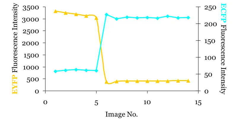
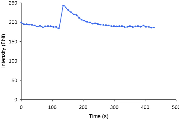
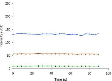
[image:34.595.105.507.464.672.2]A commonly used technique for determining FRET efficiency is acceptor photobleaching. This involves bleaching the acceptor fluorophore and monitoring donor recovery from quenching illustrated in Figure 1-4 (Wouters, Verveer et al. 2001; Pietraszewska-Bogiel and Gadella 2011). Acceptor photobleaching works on the principle that donor recovery is free from spill-over of the acceptor due to the physical properties of FP excitation. This means that donor recovery is directly related to energy transfer and number donor fluorophores in the FRET complex.
Figure 1-4. Data illustrating acceptor photobleaching.
Graphs shows spectrally deconvolved data using Zeiss linear unmixing algorithm. Acceptor
photobleaching in HeLa cell expressing ECFP-mGR and EYFP-p65 together. Acceptor EYFP is
bleached after scan 5 resulting in strong recovery of ECFP. Data provided by James Johnson.
0 500 1000 1500 2000 2500 3000 3500
0 5 10 15
Image No. E Y F P F lu or es ce n ce I n te n si ty 0 50 100 150 200 250 ECF
By using equation [III] FRET can be quickly inferred from samples, where IDD is
pre-bleached donor fluorescence in a sample and IDD’ represents a sample post acceptor
photobleaching in the same sample.
[III]
This reliance on acceptor photobleaching means that protein interactions can only be observed once in any one cell by conventional fluorophore pairs.
1.2.4.3 Artefacts and Issues
While not an issue for intramolecular biosensors and chimeric proteins such as the chameleon family of calcium sensors, fluorophore ratio can be problematic when quantifying FRET efficiency. This is manifested through intra fluorophore competition. An excess of either fluorophore can lead to nonlinear changes in efficiency. For example, if acceptor concentration exceeds that of donor concentration, competition between acceptor molecules becomes a determining factor in observed energy exchange between donor and acceptor FPs. Once acceptor molecules saturate a system, a sub-population of non-interacting acceptor molecules will be present. This means that past the point of saturation the linear relationship between sensitised emission and change in acceptor fluorescence breaks down. Although quenching will still be present, its relative change will not be proportional to changes in acceptor fluorescence. Conversely, if donor concentration exceeds acceptor concentration, sensitised emission will not correlate with acceptor fluorescence (Wouters, Verveer et al. 2001; Pietraszewska-Bogiel and Gadella 2011).
Another factor that must be taken into consideration when probing FRET results is the heterogeneity of FRET complexes in live cells. Not only can heterogeneity occur between cells, but can occur within cells. In this way it becomes important to group and visualise cell responses to FRET. For these reasons, FRET only provides a good indication of protein interaction, lack of a FRET signal does not rule out interactions as the proteins may bind to each other in a conformation where the fluorophores are
' 1
DD DD
I I
too far apart for FRET to occur. FCCS might be a strongly complementary method for FRET, and should be used in conjunction with FRET where protein interactions remain in question following FRET experiments.
1.2.5 Fluorescence Correlation Spectroscopy
Fluorescence Correlation Spectroscopy provides a different way of circumventing the conventional limit of resolution of standard microscopy. FCS works by ‘parking’ a stationary laser using X and Y galvo mirrors resulting in a small diffraction limited confocal volume placed within cell. This means that data is not raster scanned and requires the use of sensitive detectors such as avalanche photodiodes (APDs) as opposed to PMTs. The localisation and dynamics of fluorescently labelled protein can be observed by measuring the fluctuations of low numbers of fluorescent molecules as they pass through this small diffraction limited confocal volume of known size. As fluctuations in signal are detected over time, these measurements can be statistically analysed through autocorrelation analysis. Autocorrolation is defined to be (Bacia and Schwille 2007);
Where represents the lag time, and denotes averaging over time. For freely diffusing fluorophores, the following equation can be fit to describe the autocorrelation curve,
Here, the average number of fluorescent molecules in the confocal volume is represented by the term , represents the nonfluorescent component due to transitions of the fluorescent molecules through the triplet state, is the index for the diffusing species i.e. species diffusing at rate , is the relative fraction of each
[ii]
lateral ( ) radius. The characteristic diffusion time is related to the diffusion coefficient by,
[iii]
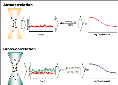
Figure 1-5 Diagrammatic representation of FCS and FCCS.
The process of forming autocorrelation (single colour) and cross-correlation (two colour) curves from
fluorescence fluctuation readings measured from individual fluorophores passing through the confocal
volume in a sample. Figure derived from Bacia et al.(Bacia, Kim et al. 2006)
Fluorescence Cross Correlation Spectroscopy (FCCS) allows the simultaneous correlation analysis of two spectrally separate fluorophores (such as DsRedExpress and EGFP). The cross-correlation curve is analogues to the autocorrelation curve but is calculated through correlating the fluorescence fluctuation profiles of the two colours (Figure 1-5), and so the cross-correlation amplitude corresponds to the degree of molecular interaction. In conjunction with the autocorrelation amplitudes, FCCS provides information on molecular binding as well as dynamic co-localisation. (Bacia, Kim et al. 2006; Kim, Heinze et al. 2007). In contrast to FRET, FCCS does not depend on the very close proximity of the interacting fluorescent labels and as a result does not require the optimisation of fluorophore orientation and linker length optimisation. However, due to imaging of a single spot, issues with regard to photobleaching makes its use to measure interactions over time limited. This makes it a good complementary method to use with FRET.
Autocorrelation
1.3 Introduction III - The NF-κB Signalling Pathway
1.3.1 NF-κB Overview
NF-κB was first discovered as a transcription factor in immune B cells and required for the transcription and translation of immunoglobulin kappa light chain gene (Sen and Baltimore 1986). NF-κB family proteins were quickly found to be a critical part of cell response to inflammation (Shakhov, Kuprash et al. 1990) apoptosis (Schauvliege, Vanrobaeys et al. 2002) and even functions not related with immune response such as neuronal embryonic development as shown in mouse embryos mediated though TRAF6 (Dickson, Bhakar et al. 2004). In fact, NF-κB dimers are shown to promote transcription of over 150 target genes (Pahl 1999). As a key transcription factor involved in so many processes, NF-κB when unchecked can lead to rheumatoid arthritis, cancer and even septic shock. The NF-κB family has garnered significant attention from the scientific community. This has resulted in significant study of how these transcription factors are controlled (Makarov 2001; Karin, Cao et al. 2002; Liu and Malik 2006).
1.3.2 NF-κB Family Members
NF-κB family members can be broadly separated into three categories (Figure 1-6). Rel proteins, Inhibitor kappa B proteins (IB) and IkappaB Kinase (IKK). Rel Proteins are the functioning transcription factors, binding to kappaB consensus sites. Mature Rel proteins consist of p65/RelA, p50/ NF-ΚB1, p52/ NF-ΚB2, RelB and c-Rel. It should be noted that p50 and p52 are formed from full length p105 and p100 respectively (Verma, Stevenson et al. 1995; Hayden, West et al. 2006).
activation, where as p65 homodimers will bind to separate transcription sites and p50 homodimers will actually inhibit transcription (Ganchi, Sun et al. 1993)
IB Proteins are somewhat more difficult to define. The IB proteins IBα, IBβ, IBε are discrete mature proteins functioning of their own volition, where as IBγ is a part of p105 and while it behaves as an inhibitor to other Rel proteins, preventing translocation into the nucleus, it can also be freely expressed in the cytoplasm of certain cells via an intronic promoter sequence. A well-characterised example in mice is expressed as a 70kDa protein (Inoue, Kerr et al. 1992), furthermore recent study has shown both IBγ and p105 to be elevated in human cases of Alzheimer ’s disease (Huang, Liu et al. 2005). p100 also possesses inhibitory behaviour for REL B (Solan, Miyoshi et al. 2002). IBζ and BCL-3 are also considered to be IB proteins due to their series of ankarin repeats consistent with IB structure, but these proteins localise to the nucleus and appear to assist p50 and p52 DNA binding (Bours, Franzoso et al. 1993; Haruta, Kato et al. 2001), though it should be noted that p50 is thought to be transcriptionally repressive. For this reason it is possible to view IB as modifiers of steady state rather than explicitly as inhibitors of nuclear translocation.
Figure 1-6. Diagram depicting NF-κB proteins
Structural domains are indicated for each family member. Rel proteins are characterised by an
N-terminal Rel Homology Domain (RHD) and a C-N-terminal Transactivation Domain (TAD). RelB
differs structurally from p65 and c-Rel due to the presence of its Leucine Zipper (LZ) domain. IκB
proteins are defined by the presence of Ankyrin Repeat Domains (ARDs), these bind RHDs of Rel
proteins and prevent nuclear localisation. The immature proteins p100 and p105 are processed to p52
and p50 respectively through the degradation of their IκB-like Ankyrin repeat domains indicated by
the arrows. Phosphorylation sites (p) shown on IκB proteins are those which target them for
degradation, phosphorylation sites shown for IKK1 and 2 are those located on the activation loop.
Unstimulated, NF-κB is sequestered in the cytoplasm in its inactive form by IB proteins (Figure 1-6). Stimuli such as TNFα or LPS activates the upstream IB kinase (IKK) complex. This complex of kinase phosphorylates the IB proteins, which are then targeted by the ubiquitin ligase machinery and degraded via the 26S proteasome. The NF-κB dimers are then free to translocate into the nucleus and bind to specific promoters where NF-κB is involved in the expression of over 150 target genes (Pahl 1999).
This general model for nuclear transduction of NF-κB uses the archetypical Rel complex p65-p50, and IBα (Nelson, Ihekwaba et al. 2004). NF-κB oscillations between cytoplasmic and nuclear compartments have been shown to be directly out of phase with the levels of IκBα (Hoffmann, Levchenko et al. 2002; Nelson, Ihekwaba et al. 2004). Through the degradation and subsequent re-synthesis of IκB, NF-κB oscillations are observed. Western blotting only measures average responses of a population, making it difficult to see asynchronous oscillations within a population of cells. For this type of study, live cell fluorescence microscopy is essential as dynamics can be tracked in the same single cell over time. This has been used to great effect in observation of oscillations in p65 localisation in live cells, as these oscillations are shown to be essential transcription of late genes such as Rantes (Nelson, Ihekwaba et al. 2004; Paszek, Lipniacki et al. 2005).
The product of the NF-ΚB1 gene p105, is shown to adhere to the principles of this model but functionally differs in key aspects. As previously mentioned, p105 is the pre-processed form of p50 containing both p50 linked by a glycine-rich region between the p50 and a C-terminal portion as described by Li Lin and Sankar Ghosh as identical to IκBγ (Lin 1996). When unprocessed, p105 remains in the cytoplasm and also complexes with p65 keeping p65 localised in the cytoplasm (Palombella, Rando et al. 1994).
proteolytic processing is by endoproteolytic cleavage followed by c-terminal degradation, or proteolysis starting at the c-terminus of p105 and terminating at the GRR sequence. It is notable that deletion of the GRR domain allowed complete proteolysis of p105 indicating its importance (Yinon and Steven 2006) (Heissmeyer, Krappmann et al. 1999; Salmeron, Janzen et al. 2001). The classic model for co-translational processing suggested by lin et.al indicates that random ribosomal pausing during translation allows the c-terminal region of p105 to undergo proteolysis via the 26s proteosome. When the ribosome does not pause, p105 cannot be processed (Lin, DeMartino et al. 1998). Other models suggests that phosphorylation of p105 by IKK leads to the ubiquitin dependent partial proteolysis of the p105 molecule leaving the p50 subunit intact thanks to the GRR region of the molecule acting as a stop signal to the proteasome. (Orian, Schwartz et al. 1999). Another possibility is the cleavage of p105 before proteolysis of the C-terminal end shown to occur at the flexible region of the GRR region between residues 430 and 465. This would imply that p50 is produced prior to degradation of the C-terminal region of p105. This has been shown by both placement of cleavage site between two stable proteins and in vitro through use of purified proteins (Lin 1996; Moorthy, Savinova et al. 2006).
Similar cleavage behaviour can be seen in the Drosophila homologue Relish. It has been shown that Drosophila IκB Kinase complex (DmIKKβ and DmIKKγ) is required for the signal-dependent proteolytic cleavage of Relish. The N terminus of Relish then translocates to the nucleus and activates the transcription of antibacterial immune response genes (Silverman, Zhou et al. 2000).
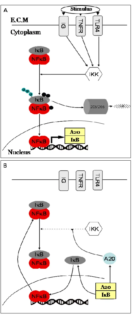
Figure 1-7 Schematic of NF-κB signalling.
NF-κB dimers translocate into the nucleus in response to an external stimulus (such as tumor necrosis
factor alpha, lipopolysaccharide or an antigen). Phosphorylation and labeling for ubiquitination of IkB
by IKK and IκB’s subsequent ubiquitin-targeted degradation allows the p50-p65 heterodimer to
translocate freely into the nucleus enabling expression of target genes. Transcription of IκB causes the
1.3.3 Multicellular Model Systems
1.4 Project Aims
The main aim of this project was to develop and apply the photoswitchable fluorescent protein Dronpa to pre-existing super resolution techniques; specifically the technique FRET. This technique is renowned for the complications introduced by spectral overlap and stoichiometric inconsistencies. Traditional fluorescent proteins do not allow the repeated probing of FRET through acceptor photobleaching due to its destructive effect on the fluorophore. By using the photoswitching properties of Dronpa, it was hoped that FRET efficiency can be repeatedly interrogated using the measure of both sensitised emission and donor quenching to help elucidate relevant and important dynamic biological functions within individual live cells over time.
It was also an aim to investigate if Dronpa could be used as a FRET partner in both mammalian and Drosophila systems, to demonstrate the flexibility of Dronpa in multiple systems. Due to the notable difference between homeostatic environments provided by the two systems this would demonstrate the utility of the technique for multiple applications. Drosophila also provide a unique system to study multicellular interactions with comparatively quick generation times compared to that of mammalian systems.
Finally, the objective was to use Dronpa in known signalling systems. Initially, it was planned to apply Dronpa-modulated FRET to the NF-B pathway. This was well characterised in mammalian cells and are readily amenable to the use of fluorescent proteins and confocal microscopy. The NF-B pathway presents many opportunities for testing protein interactions due to the dimeric nature of transcription factors and tight regulation through IkB binding and masking of transcription factor nuclear localisation sequences (NLS). It should then be possible to elucidate live cell protein interaction dynamics in single cells that occur in this pathway which have previously been shown through co-localisation of fluorophores and bulk molecular assays such as co-IPs. As a complimentary microscopy method, FCCS was also used to validate any results observed through FRET.
2.1 Materials
2.1.1 Reagents
Tissue culture medium and non essential amino acids were purchased from Gibco Life Technologies (UK) and Foetal Bovine Serum (FCS) from Harlan Seralab (UK). Human TNFα was supplied by Calbiochem (UK). Oligodeoxynucleotides were purchased from Invitrogen (UK). Schneiders S2 tissue culture media and Penicillin-Streptomycin was purchased from Gibco (UK). All other chemicals were supplied by Sigma-Aldrich (UK).
2.1.2 Expression Vectors
Expression of all mammalian fluorescent fusion protein was controlled by a cytomegalovirus (CMV) immediate-early promoter unless otherwise stated. The orientation of FP and protein of interest is always written left to right as the proteins are expressed N- to C-terminally. The expression vectors containing pp65 CDS (Clontech, UK) have been described elsewhere ((Nelson, Ihekwaba et al. 2004)) Other cDNAs used to create Gateway™ expression vectors were obtained and cloned as indicated in the appropriate following sections of this thesis. All FP fusion vectors used to create Gateway™ destination vectors were obtained from Clontech. The reading frame cassettes, employed to create destination vectors, were purchased from Invitrogen.
2.2 Molecular Biology
2.2.1 Transformation of Chemically Competent E. coli Cells
2.2.2 DNA Purification
2.2.2.1 Small Scale DNA Extraction (Mini-prep)
E.coli cells containing plasmid DNA were cultured overnight in 5ml LB broth containing an appropriate selection agent at 37°C at 230rpm. The following morning, 2ml of the stationary culture was transferred to a 2ml micro-centrifuge tube and centrifuged at 12,000g for 1min. The remaining culture was stored at 4°C for future use. The supernatant was poured off and the DNA extracted from the bacterial pellet using the Qiagen Plasmid Mini Purification Kit (Qiagen, Germany) or the GenElute Plasmid Miniprep Kit (Sigma) according to the manufacturer’s instructions. Both methods use an alkaline SDS cell lysis buffer and an acid precipitation buffer step to remove contaminating genomic DNA, and unwanted cell components. Precipitated DNA was centrifuged at 17,200xg, for 1min and the supernatant was passed through a column which adsorbed DNA onto an anion-exchange resin in the presence of high salt. After washing, the plasmid DNA was eluted in 50μl Elution Buffer (10mM Tris-HCl (pH 8.0), 1mM EDTA). Final DNA concentration was construct copy number dependent. DNA quality and identity was confirmed using an appropriate diagnostic restriction endonuclease digest followed by agarose gel electrophoresis (2.2.4).
2.2.2.2 Large Scale DNA Extraction (Maxi-prep)
E.coli cells containing plasmid DNA were cultured in a starter culture of 5 ml containing an appropriate selection for 8 h. 2ml of this culture was then used to inoculate 250ml LB broth containing an appropriate selection agent and incubated at 37°C with shaking at 230rpm for 16 h. The culture was then harvested through centrifugation at 15,000g in a bucket centrifuge for 15min at 4°C. The QIAfilter Plasmid Maxi Kit (Qiagen) or the GenElute Plasmid Maxiprep Kit (Sigma) was used in accordance with the manufacture’s guidelines. DNA eluted from the anion-exchange columns was relatively dilute and was concentrated by isopropanol precipitation. The eluted DNA solution was combined with 0.7 volumes of room-temperature isopropanol and centrifuged using a Thermoscientific CL40 SS-34 rotor at 15,000g for 30min at 4°C. The supernatant was discarded and the DNA pellets were washed by centrifugation at 15,000xg for 15min in 70% (V/V) ethanol at room
2.2.3 DNA Quantification
DNA concentration was quantified through use the Thermo Scientific NanoDrop™ 1000 Spectrophotometer. The NanoDrop uses a 1-2µl sample held in place by surface tension of the liquid. The NanoDrop measures absorbance of the sample over a 220nm-750nm spectrum reporting DNA concentration and relative purity of the sample with 230/260 and 260/280 ratio measurements. The NanoDrop was able to measure samples up to 3700µg/µl and so removed the need for serial dilution of DNA samples to ensure accurate measurment.
DNA was also semi-quantified through restriction analysis and the subsequent intensity of visualised bands compared to reference ladder concentration to confirm results of NanoDrop.
2.2.4 Restriction Endonuclease Digests
Restriction enzymes (New England Biolabs) were used to cut cDNA. Standard digestion protocol for complete digestion in a 20µl reaction volume consisted of 500ng DNA, 0.5µl restriction enzyme (RE), 1x reaction buffer (supplied) and remaining volume was made up to 20µl using MilliQ dH20. Double digest used 0.5
µl per RE. RE concentration was kept below 5% to minimize possible STAR activity of endonucleases. Digests were incubated for a minimum of 3 hr to ensure efficient digestion. Digestions were also conducted overnight if endonuclease showed low non-specific activity. In instances where buffer incompatibility meant double digests would not be feasible, products were purified using Qiagen PCR cleanup kit, as per manufacturer’s instructions, and eluted into 35l volumes. 5l of this was used between digest steps to run on an agarose gel to check digest efficiency. Previously described in house mammalian Gateway expression vectors were used as the basis for customised expression vectors (Nelson, Paraoan et al. 2002).
2.2.5 Gel Electrophoresis
run with DNA ladder HL1 (10,000-100bp) (NEB) for vectors, backbones and large PCR products. HL4 (1000-100bp) (NEB) was used for most PCR products. Gels were suspended in TAE and run at 100volts for 30 min for visualising products and 2 h at 80volts for gel extractions.
Table 2-1 Agarose Gel Percentages for DNA Fragment Separation
Gels were visualised under 302nm (UV) light using a trans-illuminator and imaged using GeneFlash with PULNiX TM-300 CCD (Syngene). Desired DNA fragments were cut from the gel by scalpel blade and purified using the QIAquick Gel Extraction Kit (Qiagen). In this protocol, agarose is dissolved to release the DNA, which is then bound to an anion-exchange membrane as used in plasmid preparation kits. Purified DNA fragment is then eluted in 30μl TE.
2.2.6 PCR and introducing Cut Sites
Polymerase Chain Reaction (PCR) and subsequent visualisation of fragments was used to confirm successful ligation of backbone and insert cDNA and success of Gateway recombination. For these diagnostic procedures, NEB Taq (1.25U/50ml) supplied with standard 10xTaq buffer was used (catalogue no. #M0273) along with 10mM NEB dNTPs (N0447L) (final concentration 100µM) and 10µM forward & reverse primer (final concentration 100nM per primer). A PCR Thermocycler px2 (ThermoScientific) using standard thermocycling conditions (as per manufactures instructions) was used for amplification. The lowest primer annealing temperature was used to determine annealing step temperature. A maximum of 30 cycles was used to amplify DNA.
Agarose in gel% w/v Best range of separation (kb)
0.3 5.0-50
0.5 1.0-25
0.8 0.7-8.0
1.0 0.5-7.0
1.2 0.4-6.0
1.5 0.2-3.0