Quantum Chemistry
Yves Alain Bernard
September 2010
A thesis submitted for the degree of Doctor of Philosophy
Declaration
This thesis contains no material which has been accepted for the award of any other
degree or diploma in any university. The work in this thesis is my own except where
otherwise stated.
Yves A. Bernard
`
First and foremost I offer my sincerest gratitude to my supervisor, Peter Gill, who
has supported me thoughout my PhD with his patience, knowledge and advice. I have
continually learnt from him and he has extended my vision of science from his clear
thoughts.
I am indebted to my many colleagues with whom I had stimulating discussions and
conducted great research. They were always available to answer my many questions. In
particular I’m grateful to Andrew, Deb, Jia and Kaew, and Titou and Josh who have
become close friends. Our office cricket games will stay in our memories. I’m grateful
to Josh and Murray who helped me correct my grammar and spelling.
I have been lucky enough to have many friends around me during my PhD, even so
far from home. I’d especially like to thank my friend from Canberra Murray, Karen,
Tony, Caitlyn, Tara, Simone, Peter and Sarah who have exposed me to Australian
culture. Maud, Titou, Julien, Lionel and Yves have kept me in contact with the French
touch and a special thought goes to Ana¨ıs. They have all been a real support to me
when work both has and hasn’t been going well. I thank Nico for having shared and sent
me music, important support for a PhD. I also received support form all my friends in
Geneva with whom I was able to stay in contact, and I express my gratitude to Gr´egory
for his unconditional support during the last days of this Thesis.
Finally I’d like to thank my parents and my sister who have supported me
through-out my continuing education. They have always encouraged me in everything I do and
it is they who have gotten me this far.
The ANU Research School of Chemistry and the Australian National
Computa-tional Infrastructure NaComputa-tional Facility are gratefully acknowledged for a PhD
scholar-ship and a generous allocation of computer time.
Abstract
The context of this Thesis is a new approach to the electron correlation problem
based on two ideas. The first idea states that the correlation energy can be
approxi-mated simply by a linear operator which contains information about both the position,
r, and the momentum, p, of an electron,i.e. a phase-space operator. The second idea proposes the use of two-electron operators, as the electron correlation occurs between
pairs of electrons.
The combination of these two ideas gave birth to Intracule Function Theory, where
intracules are two-electron distributions. To include position and momentum
infor-mation, Intracule Functional Theory uses the Wigner distribution, aquasi-phase-space
distribution, as atruephase-space distribution does not exist because of the Heisenberg Uncertainty Principle.
In this Thesis, we study two new phase-space variables, the one-particle Posmom
variable, s = r · p, and the two-particle Posmom intracule variable, x= (r1−r2)·(p1−p2), and their respective distributions, the Posmom densityS(s) and the Posmom intraculeX(x).
The one-particle Posmom variable s and its associated operator ¯s are known in
physics and have been used, for example, in the development of scattering theory.
However, they have never been used in quantum chemistry and we present, for the first
time, the quantum distributionS(s) for several relevant systems.
The two-particle equivalent variable,x, has been introduced previously in Intracule
Functional Theory and an intracule, based on the Wigner distribution, has been
pro-posed; the Dot intracule D(x). Within Intracule Functional Theory, we use the Dot
intracule to calculate the correlation energy of small atoms and molecules. Furthermore,
we derive the exact two-particle Posmom operator ¯x and its exact distribution X(x)
and show that the Dot intracule appears as an approximation of the exact Posmom
intracule.
The Posmom variables,sand x, are dot products between position and momentum
vectors and contain information about both the position and the momentum of one or
two electrons. Furthermore, the associated Posmom operators are quantum mechanical
observables, and thus respect the Heisenberg Uncertainty Principle. We show that they
are connected to types of electron trajectories and give us new information about the
behaviour of electrons. They could form the basis of a new type of spectroscopy.
This Thesis introduces the first applications of Posmom in quantum chemistry.
We first review the theory of quantum mechanics, quantum chemistry and Intracule
Functional Theory. We then present an entire development of the Posmom intracule
X(x) by starting from the simple and well known spherically averaged position and
momentum densities, followed by the new Posmom densityS(s) and the Wigner-based
Contents
Acknowledgements iv
Abstract v
List of Publications xiii
Notation xiv
1 General Introduction 1
1.1 What is Theoretical Chemistry? . . . 2
1.2 What is Quantum Chemistry? . . . 3
1.2.1 Domains of Physics Theory . . . 3
1.2.2 Quantum Chemistry . . . 6
1.3 Quantum Mechanics: Physical and Mathematical Background . . . 7
1.3.1 Discrete and Continuous Orthonormal Basis inF . . . 8
1.3.2 State Space and the Dirac Notation . . . 10
1.3.3 Representations in State Space . . . 11
1.3.4 Linear Operators and their Representation . . . 12
1.3.5 Eigenvalue, Eigenvector and Observable . . . 12
1.3.6 The Position and Momentum Representation . . . 13
1.3.7 Changing of Representation . . . 14
1.3.8 The Operators ¯r and ¯p . . . 14
1.3.9 Commutator and Conjugate Variables . . . 16
1.3.10 Heisenberg Uncertainty Principle . . . 17
1.3.11 Quantification of a Physical Quantity . . . 19
1.3.12 The Least You Need to Know About Quantum Mechanics . . . . 20
1.4 Outline and Aims of the Thesis . . . 21
2 Solving the Schr¨odinger Equation with a Single Reference 23 2.1 Separation of Space and Time . . . 25
2.2 Separation of Nuclear and Electronic Variables in Many-Body Systems 25 2.3 Hartree Product . . . 28
2.4 Slater Determinant . . . 30
2.5 Hartree-Fock Equation . . . 31
2.5.1 Matrix Elements . . . 31
2.5.2 Variational Principle, Fock Operator and the Hartree-Fock Equa-tions . . . 33
2.5.3 Restricted and Unrestricted Hartree-Fock . . . 35
2.6 Solution of the Hartree-Fock Equations . . . 36
2.6.1 The Pople-Nesbet and Roothaan-Hall Equations . . . 36
2.6.2 The Self-Consistent Field Method . . . 38
2.6.3 Form of the Atomic Orbitals: Basis Set . . . 40
2.7 Exact Wave Function and Correlation Energy . . . 41
2.7.1 Assumptions . . . 41
2.7.2 Excited Determinants . . . 42
2.7.3 Exact Wave Function and Full CI . . . 42
2.7.4 Electron Correlation . . . 43
2.7.4.1 Dynamic and Static Correlation . . . 45
2.7.4.2 Electron Correlation Pairs . . . 45
2.7.4.3 Radial and Angular Correlation . . . 45
2.8 Correlated Methods . . . 46
2.8.1 Truncated Configuration Interaction . . . 46
2.8.2 Coupled Cluster . . . 47
2.8.3 Many-Body Perturbation Theory . . . 48
2.9 Other Methods . . . 49
CONTENTS ix
2.9.1.1 Kohn-Sham Equations . . . 50
2.9.1.2 Exchange-Correlation Functional . . . 51
2.9.2 Multi-Configuration Self-Consistent Field . . . 53
2.9.3 Methods Involving the Interelectronic Distance . . . 54
2.10 The Least You Need to Know . . . 54
3 Introduction to Intracules 56 3.1 Introduction . . . 57
3.2 What is an Intracule? . . . 57
3.2.1 Position IntraculeP(u) . . . 58
3.2.2 Momentum IntraculeM(v) . . . 59
3.3 Intracules Based on the Wigner Distribution . . . 60
3.3.1 Intracules and Correlation Energy in the Helium-like Ions . . . . 60
3.3.2 Avoiding Heisenberg and the Wigner Distribution . . . 61
3.3.3 Intracule Family . . . 62
3.4 Intracule Functional Theory . . . 64
3.5 Concluding Remarks . . . 65
4 Compact expressions for spherically-averaged position and momen-tum densities 67 4.1 Introduction . . . 68
4.2 Theory . . . 69
4.2.1 Spherically-averaged position space densities . . . 69
4.2.2 Spherically-averaged momentum space densities . . . 69
4.2.3 Derivatives . . . 70
4.3 Computational Details . . . 72
4.4 Results and Discussion . . . 72
4.4.1 10-electron series . . . 72
4.4.1.1 Binding densities . . . 74
4.4.1.2 Basis set and correlation effects . . . 75
4.4.2 18-electron series . . . 77
5 Posmom: The Unobserved Observable 82
5.1 Introduction . . . 83
5.2 Posmom Theory . . . 84
5.3 Hydrogen Atom . . . 87
5.4 Lithium Hydride Molecule . . . 90
5.5 Concluding Remarks . . . 92
6 The distribution ofr·p in quantum mechanical systems 94 6.1 Introduction . . . 95
6.2 Theory . . . 97
6.2.1 Posmom Density . . . 97
6.2.2 Many-Particle Systems . . . 98
6.3 Examples . . . 99
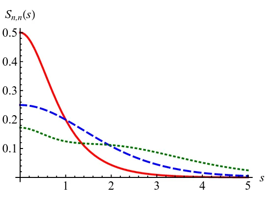
6.3.1 Harmonic Oscillator . . . 99
6.3.2 Hydrogenic ions . . . 104
6.3.3 A Particle in a Box . . . 105
6.3.4 Fermions in a Box . . . 107
6.4 Conclusions . . . 109
6.5 Acknowledgements . . . 109
7 The distribution ofr·p in atomic systems 111 7.1 Introduction . . . 112
7.2 Theory . . . 113
7.3 Hydrogenic ions . . . 115
7.4 Computational details . . . 117
7.5 Atomic orbital Posmom densities . . . 117
7.6 A model for atomic orbital Posmom densities . . . 119
7.7 The special values= 0 . . . 123
7.8 Basis effect on S(s) . . . 127
7.9 Correlation effect on S(s) . . . 128
CONTENTS xi
8 Intracule Functional Models.
III. The Dot Intracule and its Fourier Transform 134
8.1 Introduction . . . 135
8.2 The Dot Intracule and its Fourier transform . . . 136
8.3 Interpretation ofD(x) and Db(k) . . . 139
8.4 A Correlation Model based on D(x) . . . 143
8.5 A Correlation Model based on Db(k) . . . 146
8.6 Reaction energy errors . . . 148
8.7 Conclusions . . . 150
9 The distribution ofr12·p12 in quantum systems: a new exact intracule 151 9.1 Introduction . . . 152
9.2 The Posmom intracule . . . 153
9.3 Quantum dots . . . 159
9.3.1 Hamiltonian and wave functions . . . 159
9.3.2 Position Intracule . . . 162
9.3.3 Momentum Intracule . . . 162
9.3.4 Angle Intracule . . . 162
9.3.5 Dot and Posmom intracules . . . 164
9.3.6 Intracule Holes . . . 164
9.4 Helium-like ions . . . 168
9.4.1 Ground state . . . 168
9.4.2 Excited States . . . 172
9.4.3 D-dimensional helium atom . . . 173
9.5 Conclusions . . . 175
10 Conclusions and Future Directions 176 10.1 General Conclusions . . . 176
10.2 Challenge for the Posmom DensityS(s) . . . 177
10.2.1 Molecular Systems . . . 177
10.3 Challenge for the Posmom IntraculeX(x) . . . 178
A Atomic Units 179 B Expectation Values of the Hamiltonian for N = 2 180 B.1 One- and Two-Electron Integrals forN = 2 . . . 180
B.2 Integration Over the Spin Component . . . 184
C Mathematical Details of the Posmom Density Theory 187 C.1 Derivations for the ¯soperator . . . 188
C.1.1 Orthonormality . . . 188
C.1.2 Closure Relation . . . 188
C.2 Hyperbolic Autocorrelation . . . 190
C.3 Quasi-Hyperbolic Autocorrelation . . . 191
D Evaluation of Infinite Range Oscillatory Integrals: The Evans and Chung Method 192 D.1 Evaluation of Infinite Range Oscillatory Integrals . . . 193
D.2 The Evans and Chung Method . . . 193
D.2.1 General Contour . . . 195
D.2.2 The Contour for Particular Function . . . 197
D.3 Evans-Chung Method Applied to the Dot Intracule Integral . . . 198
D.3.1 Finding the Optimal Contour . . . 199
D.3.2 Upper Bounds . . . 202
D.3.3 Quadratures . . . 204
D.4 Conclusions . . . 204
E Posmom Methods in Q-Chem 206 E.1 Posmom DensityS(s) in Q-Chem . . . 207
E.2 Posmom IntraculeX(x) in Q-Chem . . . 211
List of Publications
This Thesis is a thesis by publications, and includes the following publications presented as:
Chapter 4: D. L. Crittenden and Y. A. Bernard,
“Compact expressions for spherically averaged position and momentum densities”,
J. Chem. Phys., vol. 131, p. 054110 (7pp), 2009.
Chapter 5: Y. A. Bernard and P. M. W. Gill, “Posmom: The unobserved observable”,
J. Phys. Chem. Lett, vol. 1, pp. 1254–1258, 2010.
Chapter 6: Y. A. Bernard and P. M. W. Gill,
“The distribution of r·pin quantum mechanical systems”,
New J. Phys., vol. 11, p. 083015 (15pp), 2009.
Chapter 7: Y. A. Bernard, D. L. Crittenden, and P. M. W. Gill, “The distribution of r·pin atomic systems”,
J. Phys. Chem. A, vol. 114, pp. 11984–11991, 2010.
Chapter 8: Y. A. Bernard, D. L. Crittenden, and P. M. W. Gill,
“Intracule functional models: III. The Dot intracule and its fourier trans-form”,
Phys. Chem. Chem. Phys., vol. 10, pp. 3447–3453, 2008.
Chapter 9: Y. A. Bernard, P.-F. Loos and P. M. W. Gill,
“The distribution of r12·p12 in quantum mechanical systems: a new exact intracule”,
Phys. Rev. A, to be submitted, 2011.
The choice of a thesis by publication is due to the sufficient number of publications
and the desire to develop, in the first three chapters, the general scientific knowledge
acquired and applied during the PhD, rather than adapting and/or rewriting each
publication.
We have used, in this Thesis, the following notation:
a a scalar
a a vector
A a matrix or a vector
¯
a an operator
a per electron quantity (for Chapter 7)
a∗ complex conjugate
A† conjugate transpose
f(a) a function
b
f(b) Fourier transform off(a)
Chapter 1
General Introduction
P
hilosophy[i.e., physics] is written in this grand book - I mean the universe - which stands continually open to our gaze, but it cannotbe understood unless one first learns to comprehend the language and
interpret the characters in which it is written. It is written in the language of
mathematics, and its characters are triangles, circles, and other geometrical
figures, without which it is humanly impossible to understand a single word
of it; without these, one is wandering around in a dark labyrinth.
Galileo Galilei,Il Saggiatore, Rome, 1623 [1]
T
he underlying physical laws necessary for the mathematical theory of a large part of physics and the whole of chemistry arethus completely known, and the difficulty is only that the exact
application of these laws leads to equations much too complicated to be
soluble. It therefore becomes desirable that approximate practical methods
of applying quantum mechanics should be developed, which can lead to an
explanation of the main features of complex atomic systems without too
much computation.
Paul Adrien Maurice Dirac, 1929 [2]
1.1
What is Theoretical Chemistry?
Chemistry is a science of nature concerned with the properties, composition and
structure of matter, and the changes it undergoes during a chemical reaction.
Chem-istry is included in the grand book of Galileo and can, therefore, be studied using
mathematics. This view yields the fields of physical chemistry and chemical physics‡.
These are sub-disciplines of chemistry and physics which investigate physicochemical
phenomena with the use of the laws of physics, where the laws of physics are expressed
in the language of mathematics.
Physical chemistry and chemical physics [3] contain a number of different branches
such as thermochemistry, chemical kinetics, photochemistry, electrochemistry,
spec-troscopy and quantum chemistry. Often, theoretical chemistry is viewed as another branch; however, the definition of theoretical chemistry is more general:
Theoretical chemistry is the art of applying theoretical reasoning to chemistry.
This definition can be applied to any part of chemistry, not only to physical
chem-istry. Nevertheless, theoretical reasoning includes, most of the time, the laws of physics
and/or mathematics, and thus theoretical chemistry folds into physical chemistry. It
will be this aspect of theoretical chemistry that will be used in this Thesis.
Theoretical chemistry contains different sub-branches depending on the theoretical
level used. At the lowest level, the application of classical mechanics to chemistry gives
the field of molecular dynamics and molecular mechanics. At a more complex level, there is quantum chemistry with the use of quantum mechanics and finallyrelativistic
quantum chemistry with the inclusion of relativistic effects.
At a particular level of theory, a theoretical chemist will try to develop a theoretical
model or theory which should reproduce existing resultsandbe able to predict new ones. These predicted results will be compared to new experimental measurements which will
then influence the theory through an iterative process until it reaches completeness or
sufficient accuracy.
‡
The difference between physical chemistry and chemical physics are subtle and will not be discussed
1.2. WHAT IS QUANTUM CHEMISTRY? 3
From the middle of the last century, progress in computer science has provided
support to theoretical chemists to implement their models. The application of computer
codes to chemistry is known ascomputational chemistry and represents the application
side of theoretical chemistry. Computational chemistry is not entirely within theoretical
chemistry: computational chemists routinely use theoretical models, implemented into
chemical software, in their research without being theoreticians.
1.2
What is Quantum Chemistry?
A general definition of quantum chemistry is
Quantum chemistry is the application of quantum mechanics to chemistry.
A more specific definition is given at the end of this section, but before getting into it,
it is important to understand the domain of application of quantum mechanics.
1.2.1 Domains of Physics Theory
Current knowledge indicates the existence of four different fundamental interactions:
Strong Interaction keeps atomic nucleus together, despite the repulsion between the positively charged protons;
Weak Interaction is responsible for the radioactive decays of nuclei by conversion of neutrons into protons;
Electromagnetic occurs between charged particles;
Gravitation occurs between massive particles.
At the human scale, only gravitational and electromagnetic interaction are
impor-tant and both have been subject to early models. The Newtonian mechanics [4], now
called classical mechanics [5], describe the gravitational force when particles are “heavy”
(&10−28 kg) and “slow-moving” (.108 m/s) and the Maxwell equations [6],
founda-tion of electrodynamics [7], describe the behaviour of electric and magnetic fields when
represented by the bottom-right corner in Figure 1.1. More accurate models,
depend-ing on the size and the velocity of the particles, have been developed and are discussed
below.
Velocity
Mass
RelativisticMechanics
Einstein 1905
Quantum Field Theory
Dirac 1928
Quantum Mechanics
Schrödinger 1926
Classical Mechanics
Newton 1687
~10-27kg
~10
8m/s
¯
HDψ=i∂tψ
¯
HSψ=i∂tψ F =ma
[image:19.595.195.448.192.434.2]F =mva
Figure 1.1: Domains of dynamical equations (adapted from Figure 1.2 of [8])
When the particles are “fast-moving”, the equations of classical mechanics must be
replaced by those of Einstein special [9] or general relativity [10] (see top-right corner
in Figure 1.1), where the mass becomes a function of the velocity and time, and space
form a continuous four dimension space, the spacetime continuum.
When the particles are “light”, the mechanics change from classical to quantum and
from being deterministic to probabilistic (more correctly, quantum mechanics is also
deterministic, but the interpretation is probabilistic). The equation that governs the
quantum mechanics is the Schr¨odinger equation [11] (bottom-left corner in Figure 1.1).
The Schr¨odinger equation is presented in the next Subsection and is the subject of
1.2. WHAT IS QUANTUM CHEMISTRY? 5
When the particles are, at the same time, “light” and “fast-moving” (see top-left
corner in Figure 1.1), both quantum and relativistic effects are important. In relativistic
quantum chemistry the Schr¨odinger equation is replaced by the Dirac equation [12].
More complex models exist with the inclusion of the weak and the strong
interac-tions. Quantum electrodynamics (QED) [13] is the unified theory of the weak and the
electromagnetic forces. Similarly, the strong interaction can be coupled with QED into
a single model. This model is known as the standard model of particle physics. It is
a quantum field theory which is compatible with the principles of quantum mechanics
and of relativity. It is the most complete theory of matter ever produced; however it is
not the final one, as it does not include the gravitational interaction. The current hope
of such a grand unified theory relies on string theory, which holds the greatest promise.
There are two well-written books for the general public on the subject [14, 15].
To illustrate these different models, we can look at their prediction of the Land´e
factor or g-factor of the electron. The g-factor is a dimensionless quantity which
char-acterizes the magnetic moment and gyromagnetic ratio of a particle or nucleus. For
example, the electron has a magnetic moment of modulus ege~/(4mec) (symbols are defined in Appendix A). While classical electrodynamics erroneously suggests ge = 1
and the standard quantum mechanics of the Schrodinger equation is not able to derive
a value ofge, the Dirac equation predicts a value forge= 2 exactly [13]. However there
exists a small deviation, a= (g−2)/2, as first measured in 1947 [16], and the current experimental deviation is [17]
aexp '0.001 159 652 180 85(76).
This small deviation is perfectly understood within QED which predicts [18]
ath '0.001 159 652 153 5(240)
The agreement between theory and experiment to a level of 10 decimal figures is
1.2.2 Quantum Chemistry
Understanding electron motion and behaviour in atoms and molecules is a key part
of chemistry. Electrons have a small mass (9.11×10⁻³¹ kg) and quantum mechanics must be employed to describe their motion. At low velocity, which is the case of
electrons in an atom of the top half of the periodic table of elements, the relevant
equation is the time-dependent Schr¨odinger equation
¯
HSΨ(r, t) =i~∂Ψ(r, t)
∂t , (1.1)
where Ψ(r, t) is the time-dependent position wave function andHS¯ is the Schr¨odinger
Hamiltonian operator given by the sum of the kinetic, ¯T, and potential, ¯V, energy
operators
¯
HS = ¯T+ ¯V
= p¯ 2 2m + ¯V
=−~ 2 2m∇
2+V(r, t). (1.2)
In the last line, the operators are expressed in the position representation (see
Sec-tion 1.3.8) and ∇ is the vector gradient. The wave function, solution of (1.1), is
connected to the probabilityP(r, t) of observing a particle at the positionrand time
tvia its squared modulus
P(r, t) =|Ψ(r, t)|2. (1.3) If the electrons are moving at a velocity close to the speed of light (c = 3.00× 10⁸ m/s) such as in atoms of the bottom half of the periodic table of elements, the Schr¨odinger equation is replaced by the Dirac equation, which is formally of the same
form as (1.1) – but the Dirac Hamiltonian is more complicated. As a result, the
relativistic wave function solution has four components. Without getting into details,
the Dirac Hamiltonian is
¯
1.3. QUANTUM MECHANICS:
PHYSICAL AND MATHEMATICAL BACKGROUND 7
With the formulation of this equation, Dirac established the basis of quantum
chem-istry as described in the quote at the beginning of this chapter. It can be summarized
as
Quantum chemistry is the art of applying approximation to the solution of the Schr¨odinger or Dirac equations.
In a very few cases, such as the Hydrogen atom, both equations can be solved in
closed form and produce results in terms of analytical functions [13].
1.3
Quantum Mechanics:
Physical and Mathematical Background
Quantum mechanics is a difficult theory and this section presents only some basic
physical and mathematical aspects of it used during this PhD. A complete introduction
can be found in the books of Cohen-Tannoudji et al. [19, 20] from which this section is based. The presentation below does not follow the historical emergence of quantum
mechanics, as it is probably as complex as the theory itself [21], and no attempt is
made here to be rigorous or complete.
We have already introduced the time dependent position wave function Ψ(r, t), the
equation describing its evolution (1.1) (the Schr¨odinger equation) and its probabilistic
interpretation (1.3). We shall now be more precise:
• For the classical concept of trajectory, we must substitute the concept of time-varying state. The wave function Ψ(r, t) characterizes the quantum state of a particle such as an electron and it contains all information it is possible to obtain
about the particle.
• The total probability of finding the particle somewhere in space is equal to 1, so we must have
Z
• The result of a measurement of an arbitrary physical quantity must belong to a set of eigenvalues {a}.
• Each eigenvalue a is associated with an eigenstate ψa(r) ∈ F. This function is such that, if Ψ(r, t0) =ψa(r), where t0 is the time at which the measurement is performed, the measurement will always bea.
• For any Ψ(r, t), the probabilityP(a) of finding the eigenvalueafor the measure-ment at time t0 is found by decomposing Ψ(r, t0) in terms of functionsψa(r)
Ψ(r, t0) =X a
caψa(r), (1.6)
then
P(a) = |ca| 2
P
a|ca|2
and X a
P(a) = 1. (1.7)
1.3.1 Discrete and Continuous Orthonormal Basis in F
We are now considering the wave function at time t0 and use the short notation
ψ(r) = Ψ(r, t0). The decomposition (1.6) corresponds to expressing the wave function in a basis. The set {fi(r)}is orthonormal if
(fi, fj)≡
Z
fi∗(r)fj(r)dr=δi,j, (1.8)
where we have introduced the scalar product (fi, fj) and δi,j is the Kronecker delta
function. Furthermore, if the set {fi(r)} is complete – i.e. it satisfies the closure relation
X
i
fi∗(r)fi(r0) =δ(r−r0), (1.9) whereδ(r) is the Dirac delta function – it constitutes abasis. Therefore every function
ψ(r)∈F can be expanded in one and only one way in terms of thefi(r)
ψ(r) =X
i
cifi(r). (1.10)
The componentci of ψ(r) on fi(r) is equal to the scalar product
ci= (fi, ψ) =
Z
1.3. QUANTUM MECHANICS:
PHYSICAL AND MATHEMATICAL BACKGROUND 9
and the scalar product between two wave functions ψ(r) and ϕ(r) expressed in the
basis
ψ(r) =X
i
cifi(r) and ϕ(r) =X
i
bifi(r) (1.12)
is
(ϕ, ψ) =X i
b∗ici (1.13)
and in particular
(ψ, ψ) =X i
|ci|2. (1.14)
The generalization of the above relations to a continuous basis is straightforward.
We need to replace the discrete index i by a continuous index α, the sum over the
indexi by an integral over α and the Kronecker delta function δi,j by the Dirac delta
function δ(α−α0). In a continuous basis, the orthonormal relation (1.8), the closure relation (1.9) and the wave function development (1.10) become
Z
fα∗(r)ψα0(r)dr=δ(α−α0) (1.15)
Z
fα∗(r)fα(r0)dα=δ(r−r0) (1.16)
ψ(r) =
Z
c(α)fα(r)dα, (1.17)
The most trivial basis is when the continuous index is a vector positionα=r0 with
fr0(r) =δ(r−r0)) (1.18) c(r0) =ψ(r0) (1.19)
and it is certainly true that any function can be written as
ψ(r) =
Z
ψ(r0)δ(r−r0)dr0, (1.20) with the componentψ(r0) given by
ψ(r0) = (fr0, ψ) =
Z
fr∗0(r)ψ(r)dr (1.21)
Therefore the probability of finding the particle at r0 is given, as expected (1.3), by the squared modulus of the componentψ(r0)
It is possible to develop a wave function within a basis of elements that do not
belong toF. For example, if the continuous index is the vector momentumα=p0 (we anticipate here the physical meaning of the index), the set of functions
gp0(r) = (2π~)
−3/2eip0·r/~ (1.23)
forms a basis and there exists a unique decomposition such that
ψ(r) =
Z
φ(p)gp0(r)dp0 (1.24)
= (2π~)−3/2
Z
φ(p0)eip0·r/~dp0 (1.25)
and
φ(p0) = (gp0, ψ) =
Z
gp∗0(r)ψ(r)dr (1.26)
is the momentum wave function. Equation (1.25) corresponds to a Fourier transform
and yields an important result of the quantum mechanics: the position wave function
is connected to the momentum wave function via a Fourier transform. This property will be used later to derive other important relations such as the momentum operator
in position representation or the Heisenberg uncertainty principle.
1.3.2 State Space and the Dirac Notation
At the beginning of this section, we stated that the quantum state of a particle
is defined, at a given time, by a wave function ψ(r) ∈ F. This wave function can be represented by several distinct sets of components, each one corresponding to the choice
of a basis. We now generalize the notion of state:
• The quantum state of any physical system is characterized by a state vector, belonging to a space Ewhich is the state space of the system. E is a subspace of a Hilbert space and is isomorphic withF.
Any element, or vector, of E, is called a ket and is represented by the symbol|ψi with the relation
1.3. QUANTUM MECHANICS:
PHYSICAL AND MATHEMATICAL BACKGROUND 11
For every ket vector there exists an adjoint vector called a bra, represented by the
symbolhψ|and hψ| ∈E∗, whereE∗ is the dual space of E.
The scalar product between two kets, |ψi and |ϕi is defined as
(|ϕi,|ψi) =hϕ|ψi (1.28) where hϕ|ψi is called the Dirac notation of the scalar product. We summarize below the properties of the scalar product using the Dirac notation
hϕ|ψi=hψ|ϕi∗ (1.29) hϕ|λ1ψ1+λ2ψ2i=λ1hϕ|ψ1i+λ2hϕ|ψ2i (1.30) hλ1ϕ1+λ2ϕ2|ψi=λ∗1hϕ1|ψi+λ∗2hϕ2|ψi (1.31) hψ|ψireal, positive; zero if and only if |ψi= 0 (1.32) whereλi is a complex number.
1.3.3 Representations in State Space
A set of discrete kets {|fii} is said to be orthonormal if the kets of this set satisfy the orthonormalization relation
hfi|fji=δi,j. (1.33) The set {|fii}constitutes a basis if every ket |ψi ∈E has a unique expansion on the |fii
|ψi=X i
ci|fii, (1.34)
which implies the following closure relation (or completeness)
X
i
|fii hfi|= ¯1, (1.35)
where ¯1 denotes the identity operator inE. Using (1.33), we obtain the expression for the componentscj of the vector|ψi in the representation{|fji}
1.3.4 Linear Operators and their Representation
A linear operator ¯Aassociates with every ket|ψi ∈Eanother ket|ψ0i ∈Ethrough a linear correspondence
¯
A|ψi=
ψ0
. (1.37)
Given a representation such as {|fii}, we can associate a series of numbers to the operator ¯A
Ai,j =hfi|A¯|fji. (1.38) As these numbers depend on two indices, we refer to them as matrix elements of ¯A.
The product of two linear operators ¯A and ¯B, is defined as
¯
AB¯|ψi= ¯A( ¯B|ψi). (1.39) In general, ¯AB¯ 6= ¯BA¯ and we define the commutator between two operators¯
A,B¯
as
¯
A,B¯
= ¯AB¯−B¯A.¯ (1.40)
1.3.5 Eigenvalue, Eigenvector and Observable
The ket vector |ψi is said to be an eigenvector of the linear operator ¯Aif ¯
A|ψi=λ|ψi, (1.41) whereλis a complex number and is called the eigenvalue of |ψi.
A very important class of operator is when ¯Ais Hermitian, i.e. when the operator is equal to his adjoint, ¯A = ¯A†. Let {a
i} and {|fii} be the sets of eigenvalues and eigenvectors of the Hermitian operator ¯A (we consider no degeneracy) such that
¯
A|fii=ai|fii. (1.42) It is easy to show that all eigenvalues ai are real and two eigenvectors with different
eigenvalues are orthogonal
1.3. QUANTUM MECHANICS:
PHYSICAL AND MATHEMATICAL BACKGROUND 13
The Hermitian operatorA¯is anobservableif its set of orthonormal eigenvectors form a basis in the state space.
1.3.6 The Position and Momentum Representation
In Section 1.3.1 we introduced two particular bases of F, {fr0(r)} and {gp0(r)}
composed of functions
fr0(r) =δ(r−r0) (1.44) gp0(r) = (2π~)
−3/2eip0·r/~ (1.45)
such that any function in F can be expanded in one or the other of these bases. The ket associated with fr0(r) and gp0(r) are denoted |r0i and |p0i, respectively and the
coefficients hr0|ψi and hp0|ψiare hr0|ψi=
Z
fr∗0(r)ψ(r)dr=ψ(r0) (1.46)
hp0|ψi=
Z
gp∗0(r)ψ(r)dr=φ(p0), (1.47)
whereφ(p) is the Fourier transform of ψ(r).
The value ψ(r0) of the wave function at the pointr0 is thus shown to be the component of the ket |ψi on the basis vector |r0i of the {|r0i} representation.
A similar interpretation applies to the wave function in momentum spaceφ(p).
Now that we have reinterpreted the wave function ψ(r) and its Fourier transform
φ(p), we will denote the basis vector of these two representations by|riand|piinstead of |r0i and |p0i, and
For the position and momentum representation, the orthonormalization and closure
relations are the generalizations of (1.33) and (1.35) and read
hr|r0
=δ(r−r0) (1.50) hp|p0
=δ(p−p0) (1.51)
Z
|ri hr|dr= ¯1 (1.52)
Z
|pi hp|dp= ¯1. (1.53)
1.3.7 Changing of Representation
A given ket |ψi is represented by (1.48) in the position representation |ri and by (1.49) in the momentum representation |pi. To change from the|ri representation to|pi representation, requires the numbers
hr|pi=
Z
fr∗(r0)gp(r0)dr0 = (2π~)−3/2eip·r/~. (1.54)
Using the closure relation (1.51), we find
hr|ψi=
Z
hr|pi hp|ψidp, (1.55) which is
ψ(r) = (2π~)−3/2
Z
φ(p)eip·r/~dp. (1.56)
Inversely, we have
hp|ψi=
Z
hp|ri hr|ψidr, (1.57) which is
φ(p) = (2π~)−3/2
Z
ψ(r)e−ip·r/~dr. (1.58)
The above relations recall the known result of the relation between the position and
the momentum wave functions.
1.3.8 The Operators r¯ and p¯
1.3. QUANTUM MECHANICS:
PHYSICAL AND MATHEMATICAL BACKGROUND 15
components (¯x,y,¯ z¯) and (¯px,p¯y,p¯z), respectively, such that
¯
r|ψi=r|ψi (1.59) ¯
p|ψi=p|ψi (1.60) and in particular
¯
x|ψi=x|ψi ; px¯ |ψi=px|ψi (1.61) ¯
y|ψi=y|ψi ; py¯ |ψi=py|ψi (1.62) ¯
z|ψi=z|ψi ; pz¯ |ψi=pz|ψi. (1.63) The matrix elementshϕ|r¯|ψiandhϕ|p¯|ψican easily be determined within the position and the momentum representation using the closure relation (1.52) and (1.53)
hϕ|r¯|ψi=
Z
hϕ|ri hr|r¯|ψidr=
Z
ϕ∗(r) rψ(r)dr (1.64)
hϕ|p¯|ψi=
Z
hϕ|pi hp|p¯|ψidp=
Z
χ∗(p)p φ(p)dp, (1.65)
where χ(p) is the Fourier transform of ϕ(r). We now want to express the operator ¯p
in the position representation. Let’s first look at the component ¯px
hr|px¯ |ψi=
Z
hr|pi hp|px¯ |ψidp= (2π~)−3/2
Z
eip·r/~ px φ(p)dp. (1.66)
We recognize the Fourier transform of pxφ(p), which is −i~∂∂xψ(r) (see Appendix I
in [20]). Therefore
hr|p¯|ψi=−i~∇hr|ψi (1.67) and the matrix element (1.65) can now be expressed in the position representation
hϕ|p¯|ψi=
Z
hϕ|ri hr|p¯|ψidr=
Z
ϕ∗(r) (−i~∇)ψ(r)dr. (1.68) Similarly, the operator ¯r in the momentum representation is
hp|r¯|ψi=i~∇hp|ψi (1.69) Most of the time, physicists work in the position representation and use the short
hand notation
¯
r=r (1.70)
¯
such as in (1.2).
It is easy to show that the operator ¯r and ¯pare Hermitian and their eigenvectors,
|ri and |pi, form a basis in E. Therefore, ¯r and ¯p are observable and correspond, of course, to the position and momentum of the particle, respectively.
1.3.9 Commutator and Conjugate Variables
Since we have the form of the momentum operator in the position representation,
we can now calculate the commutator (1.40) between the components of ¯rand ¯p. For
example
hr|[¯x,px¯ ]|ψi=hr|x¯px¯ −px¯ x¯|ψi =xhr|p¯x|ψi+i~∂
∂xhr|x¯|ψi =−i~x ∂
∂xhr|ψi+i~
∂
∂x xhr|ψi
=−i~x ∂
∂xhr|ψi+i~hr|ψi+i~x
∂
∂x hr|ψi
=i~hr|ψi. (1.72)
This is true for any ket|ψiand, in the same way, we find all other commutators between the components of ¯r and ¯p
[¯i,¯j] = 0 (1.73)
[¯pi,pj¯ ] = 0 (1.74)
[¯i,pj¯ ] =i~δi,j, (1.75)
fori, j=x, y, z.‡
Two observables, ¯A and ¯B, whose commutator is ¯
A,B¯
=i~, are said to be
con-jugate variables. It can be shown (see Complement EII in [19]) that their eigenvectors are connected via a Fourier transform. We already saw that position and momentum
are conjugate variables. Another couple is, for example, time and energy.
‡
We should keep in mind that the commutator between two operators is also an operator and the
1.3. QUANTUM MECHANICS:
PHYSICAL AND MATHEMATICAL BACKGROUND 17
1.3.10 Heisenberg Uncertainty Principle
In 1927, Heisenberg derived, from quantum mechanics, a fundamental physical
prop-erty called the Heisenberg Uncertainty Principle [22]. Before this discovery, it was thought that the precision of any measurement was limited only by the accuracy of the
experimental instruments used. However, Heisenberg showed that quantum mechanics
limits the precision of simultaneous measurement of some properties, whatever the
ex-perimental precision. The properties that cannot be known at the same time with an
arbitrary precision are couples of conjugate variables.
We give here a general derivation of the Heisenberg Uncertainty Principle. Let ¯Q
and ¯P be two observables with commutator ¯
Q,P¯
=i~. For example, the mean value of ¯Qis defined as
hQi=hψ|Q¯|ψi (1.76) and its root-mean-square deviation as
∆Q=
q
hψ|( ¯Q− hQi)2|ψi=
q
hQ2i − hQi2. (1.77) Consider the ket of the form
|ϕi= ( ¯Q+iλP¯)|ψi, (1.78) whereλ is an arbitrary real parameter. For allλ, the scalar product hϕ|ϕi(square of the norm of |ϕi) is always positive (1.32) and
hϕ|ϕi=hψ|( ¯Q−iλP¯)( ¯Q+iλP¯)|ψi
=hψ|Q¯2|ψi+hψ|iλQ¯P¯−iλP¯Q¯|ψi+hψ|λ2P¯2|ψi =
Q2
+iλ¯
QP¯
+λ2
P2
=
Q2
−λ~+λ2P2≥0. (1.79) The discriminant of this expression, second order in λ, must be negative or zero
~2−4P2 Q2≤0 (1.80) and we have
P2 Q2
≥ ~ 2
Assuming|ψi to be given, let us introduce the two observables ¯Q0 and ¯P0 such that ¯
Q0 = ¯Q− hQi, (1.82) ¯
P0 = ¯P− hPi. (1.83) Since ¯Q0 and ¯P0 are conjugate variables
¯
Q0,P¯0
=¯
Q,P¯
=i~, (1.84)
equation (1.81) applies as well to ¯Q0 and ¯P0
P02 Q02
≥ ~ 2
4 . (1.85)
Using the definition of the root-mean-square deviation (1.77) along with (1.82) and (1.83),
we find
∆Q=phQ02i (1.86) ∆P =phP02i. (1.87) The relation (1.84) can therefore also be written
∆Q∆P ≥ ~
2, (1.88)
which is the Heisenberg Uncertainty Principle. The special case where ¯Q = ¯r and
¯
P = ¯pyields the most well known form of the Heisenberg Uncertainty Principle
∆x∆px≥ ~
2, ∆y∆py ≥ ~
2 and ∆z∆pz ≥ ~
2. (1.89)
Thus the position and the momentum of a particle cannot be known simultaneously
with arbitrary precision. There exists a lower bound for the product ∆r∆p which
depends on the fundamental reduced Planck constant~= 1.05457168(18)×10−34 J s. The generalization of (1.88) to two arbitrary observables ¯Aand ¯B yields
∆A∆B ≥ 1 2
¯
A,B¯
. (1.90)
The reduced Planck constant has a very low numerical value and only becomes
important when the size of the system is small, such as an electron. That is why the
Heisenberg Uncertainty Principle does not apply at human scale. Thus, the concept
of trajectory, the knowledge ofr and pat any time, is still very important in classical
mechanics, but must be abandoned in the discussion of electron motion. In the limit
1.3. QUANTUM MECHANICS:
PHYSICAL AND MATHEMATICAL BACKGROUND 19
1.3.11 Quantification of a Physical Quantity
We discuss here how to construct the observable (operator) ¯A which describes, in
quantum mechanics, the physical quantity A defined in classical mechanics.
For a single particle, without spin, subject to a scalar potential, any physical
quan-tity Arelated to it is expressed in terms of the fundamental dynamical variablesrand
p, thusA=A(r,p, t). We already know that the positionr(x, y, z) and the momentum
p(px, py, pz) of a particle are associated with the operators ¯r(¯x,y,¯ z¯) and ¯p(¯px,py,¯ pz¯ ),
respectively. To obtain the corresponding observable ¯A, one could simply replace, in
the expression forA(r,p, t), the variablesr and pby the observables ¯r and ¯p
¯
A(t) =A(¯r,p¯, t). (1.91) However, this mode of action would be ambiguous in general. Assume, for example,
that
A(r,p, t) =r·p=xpx+ypy+zpz. (1.92) In classical mechanics, the scalar product is commutative
r·p=p·r (1.93)
but the corresponding operators are not
¯
r·p¯6= ¯p·r¯. (1.94) Moreover, neither ¯r·p¯nor ¯p·r¯ is Hermitian. To the preceding postulate, one must add a symmetrization rule and yield the following postulate: the observable ¯A which
describes a classically defined physical quantity A is obtained by replacing, in the suitablysymmetrized expression forA,randpby the observables ¯rand ¯p, respectively.
For example, the observable associated with r·pis 1
2(¯r·p¯+ ¯p·r¯) (1.95) which is indeed Hermitian.
We note that there exists quantum physical quantities which have no classical
equiv-alent and are therefore defined directly by the corresponding observable. This is the
1.3.12 The Least You Need to Know About Quantum Mechanics
The principles of quantum mechanics described in this section can be summarized
by the seven postulates given in Chapter III of [19].
Description of the State of a System: At a fixed time t0, the state of a physical system is defined by specifying a ket |ψ(t0)i belonging to the state spaceE. Description of Physical quantities: Every measurable physical quantity A is
de-scribed by an Hermitian operator ¯A acting in E, whose eigenfunctions form a complete set (a basis) inE; this operator is an observable.
Quantization Rules: The observable ¯A, which describes a classically defined physical quantity A, is obtained by replacing r and p with the observables ¯r and ¯p, respectively, in the suitably symmetrized expression forA.
Measurement of a Physical Quantities: The only possible result of the measure-ment of a physical quantity A is one of the eigenvalues of the corresponding observable ¯A.
Principle of Spectral Decomposition (case of discrete spectrum): When the phys-ical quantity A is measured on a system in the normalized state |ψi, the prob-ability P(a) of obtaining the eigenvalue a of the corresponding observable ¯A
is
P(a) =|hfa|ψi|2, (1.96) where|fai is the normalized eigenvector of ¯A associated with the eigenvaluea.
Principle of Spectral Decomposition (case of continuous spectrum): When the physical quantity A is measured on a system in the normalized state |ψi, the probability dP(α) of obtaining a result included betweenα and α+dα is
dP(α) =|hfα|ψi|2dα, (1.97) where|fαi is the eigenvector corresponding to the eigenvalueα of the observable
¯
1.4. OUTLINE AND AIMS OF THE THESIS 21
Reduction of the Wave Packet: If the measurement of the physical quantityAon a system in the state |ψi gives the resultα, the state of the system immediately after the measurement is the eigenvector|fαiassociated with α.
Time Evolution of systems: The time evolution of the state vector |ψ(t)i is gov-erned by the Schr¨odinger equation
i~∂
∂t|ψ(t)i= ¯H(t)|ψ(t)i, (1.98) whereH¯ is the observable associated with the total energy of the system.
¯
H(t)|ψ(t)i=E(t)|ψ(t)i. (1.99)
1.4
Outline and Aims of the Thesis
This general introduction has described the field of this Thesis and has presented
the background of quantum mechanics. From the postulates of quantum mechanics,
summarized in the previous section, the quantization rules and the measurement of
physical quantities, will be used in Chapters 5, 6 and 9.
Chapter 2 presents the heart of quantum chemistry, which consists of applying
approximation to the solution of the Schr¨odinger equation. The Hartree-Fock method
is then derived in detail, and common post Hartree-Fock or correlated methods are
reviewed.
Chapter 3 introduces intracules,i.e.two-particle probability densities, and the gen-eral concept of Intracule Function Theory (IFT) is exposed. IFT uses Wigner-based
intracules which do not respect entirely the Heisenberg Uncertainty Principle. At the
end of the chapter, a specific question is asked, which corresponds to the general aim
of this Thesis: Can we construct an intracule which contains information on both the
position and the momentum of particleswithout the use of a quasi-phase-space
distri-bution, while respecting the principles of quantum mechanics such as the Heisenberg
Uncertainty Principle?
Chapters 4 to 8 explain the method used to answer this question, and a solution is
proposed in Chapter 9.
Chapter 4 starts by describing the spherically-averaged position and momentum
Chapter 5 discusses a new dynamical variable (the Posmom) which provides new
insights on electron motion and could – we assert – form the basis of a new type of
spectroscopy. The Posmom lies between the position and the momentum and we show
all the relations between these three quantities. We illustrate the physical significance
of this observable in the case of the hydrogen atom and the lithium hydride molecule.
Chapter 6 goes into the mathematical details behind the Posmom observable and
its quantum density. Several quantum mechanical systems are analyzed such as the
harmonic oscillator, particles in a box and hydrogenic ions.
Chapter 7 corresponds to the application of Posmom density to atomic systems.
We looked at the ground states of the 36 lightest atoms and we have decomposed the
total Posmom density into atomic orbital contributions.
Chapter 8 describes the Wigner-based Posmom intracule, called Dot intracule and
it is used, within IFT, to determine the correlation energy of several atoms and small
molecules.
Chapter 9 introduces a new exact intracule, the Posmom intracule which contain
information on both the relative position and momentum of electron pairs. The
Pos-mom intracule is compared with other intracules in the simple case of two particles in
a three-dimensional harmonic well. Different excited states and dimensionality of the
helium atom are also investigated with the Posmom intracule.
Finally, Chapter 10 lays out the main conclusions and suggests future directions for
this work.
Chapter 2
Solving the Schr¨
odinger Equation
with a Single Reference
Solving the Schr¨odinger equation is the heart of quantum chemistry. This chapter
presents the problem of the quantum many-electron system. It discusses the structure
of the Hamiltonian for such a system and introduces the basic ideas of the Hartree-Fock
approximation as well as post-Hartree-Fock methods.
Hartree-Fock theory [23, 24] describes the simplest approximate method to
deter-mine the ground-state wave function and ground-state energy of a quantum many-body
system. In chemistry, it is the foundation of molecular orbital theory.
After separating space and time (stationary states), Section 2.1, and the nuclear and
electronic variables (Born-Oppenheimer approximation), Section 2.2, of the Schr¨odinger
equation, the main approximation describes each electron’s motion by a single-particle
function (spin orbital), Section 2.3, which does not depend explicitly on the
instanta-neous motions of the other particles. Each electron “sees” only the average potential of
the others electrons. Hence, Hartree-Fock theory is also referred to as an independent
particle model ormean field theory.
The second approximation assumes that the exact many-body wave function of a
system can be approximated by a single Slater determinant of N spin orbitals,
Sec-tion 2.4. Finally, the spatial component of each spin orbital is expanded within a basis
of known functions (linear combination of atomic orbital approximation) in Section 2.6.
The consequences of the approximations in the Hartree-Fock method are exposed
in Section 2.7 and some post Hartree-Fock methods are presented in Section 2.8.
Sections 2.2 to 2.7 of this chapter follow Szabo and Ostlund [25], and Section 2.8
2.1. SEPARATION OF SPACE AND TIME 25
2.1
Separation of Space and Time
The time-dependent Schr¨odinger equation is given by (1.1). For bound systems
where the potential energy operator is time-independent, V(r, t) = V(r), the
Hamil-tonian operator also becomes time-independent, H¯=H¯(r). When it acts on a wave
function, it yields the total energy E(r), which depends only on the position
¯
H(r)Ψ(r, t) =E(r)Ψ(r, t) (2.1)
=i~∂Ψ(r, t)
∂t . (2.2)
The solution of this first order differential equation
Ψ(r, t) = Ψ(r)e−iEt (2.3)
shows that the time and space variables of the wave function can be separated and
that the time dependence is given by a simple multiplicative phase factor. For
time-independent problems, this phase factor is normally neglected, and the starting point
is taken as the time-independent Schr¨odinger equation
¯
H(r)Ψ(r) =E(r)Ψ(r). (2.4)
In the simplerDirac notation it reads
¯
H |Ψi=E|Ψi. (2.5)
2.2
Separation of Nuclear and Electronic Variables in
Many-Body Systems
Unlike Hydrogenic systems, if there is a second electron around the nucleus, the
problem becomes inextricable and an exact solution of the Schr¨odinger equation
can-not be obtained. However, it is possible to reduce the complexity of the problem by
separating some of the space coordinates.
The time-independent Schr¨odinger equation of a system of N electrons moving
aroundMnuclei, withrdenoting electronic andRdenoting nuclear spatial coordinates,
is
¯
For such a system, the Hamiltonian H¯ is composed of five terms: the kinetic energy
operators of the electrons ¯Te(r) and of the nuclei ¯Tn(R); the Coulomb repulsion
oper-ator between electrons ¯Vee(r) and between nuclei ¯Vnn(R); and the Coulomb attraction
operator between electrons and nuclei or nuclei potential ¯Vne(r;R), or
¯
H(r,R) = ¯Te(r) + ¯Tn(R) + ¯Vne(r,R) + ¯Vee(r) + ¯Vnn(R). (2.7)
Choosing an arbitrary reference system, as shown in Figure 2.1, the distance between
theith electron and theAth nucleus isriA=|riA|=|ri−RA|; the distance between the ith andjth electron isrij =|rij|=|ri−rj|; and the distance between theAth andBth nucleus isRAB =|RAB|=|RA−RB|. Within this notation, the Hamiltonian (2.7) is
¯ H =−
N
X
i=1
1 2∇
2
i −
M
X
A=1
1 2MA
∇2A−
N
X
i=1
M
X
A=1
ZA
riA +
N
X
i=1
N
X
j>i 1 rij
+ M
X
A=1
M
X
B>A
ZAZB
RAB
, (2.8)
where MA is the ratio of the mass of nucleus A to the mass of an electron, and ZA is the atomic number of the nucleus A. The Laplacian operators ∇2
i and ∇2A involve differentiation with respect to the coordinates of the ith electron and Ath nucleus.
0
x
y z
A
B
i
j
RAB=RA−RB
RA
RB
rjA=rj−RA
riA=ri−RA
rij=ri−rj
rj
ri
Figure 2.1: The molecular coordinate system in an arbitrary reference system: i, j =
electrons; A, B= nuclei (adapted from Figure 2.1 of [25]).
One can simplify the Hamiltonian (2.8) if one compares the electron massmeto the
2.2. SEPARATION OF NUCLEAR AND ELECTRONIC VARIABLES IN
MANY-BODY SYSTEMS 27
they move more slowly. A good approximation is made if one considers the nuclei as
fixed and the electrons as moving around them. Such approximation was first proposed
by Born and Oppenheimer [26] in 1927 and is known as the Born-Oppenheimer (BO)
approximation. Within the BO approximation, the kinetic energy of the nuclei can
be neglected and the Coulomb repulsion between the nuclei can be considered to be
constant. Any constant added to an operator will not change the eigenfunction but
only add a constant to the eigenvalues. The remaining terms in (2.8) are called the
electronic Hamiltonian
¯
Helec =− N
X
i=1
1 2∇
2
i −
N
X
i=1
M
X
A=1
ZA
riA +
N
X
i=1
N
X
j>i 1
rij. (2.9)
Now, the total wave function is broken into its electronic and nuclear (vibration,
rota-tion and translarota-tion) components
Ψtotal= Ψelec×Ψnucl, (2.10)
with
¯
H(r,R)Ψtotal(r,R) =EtotalΨ(r,R). (2.11)
With the electronic Hamiltonian (2.9), one can write the electronic Schr¨odinger
equa-tion
¯
Helec(r;R)Ψelec(r;R) =Eelec(R)Ψ(r;R) (2.12)
where the electronic wave function Ψelec(r;R) describes the motion of the electrons
and depends explicitly on the electronic coordinate r but depends parametrically on
the nuclear coordinates R. By a parametric dependence we mean that, for a different
arrangements of the nuclei, Ψelec is a different function of the electronic coordinate r.
The nuclear coordinatesR do not appear explicitly in Ψelec. The total energy is given
by the sum of the electronic energy and the nuclear repulsion
Etotal=Eelec+
M
X
A=1
M
X
B>A
ZAZB
RAB
. (2.13)
Without giving many details, one can define a nuclear Hamiltonian
¯
Hnucl=− M
X
A=1
1 2MA
and a nuclear Schr¨odinger equation
¯
Hnucl(R)Ψnucl(R) =EnuclΨ(R), (2.15)
which describe the vibration, rotation and translation of a molecule. Solving the
nu-clear Schr¨odinger equation is not the purpose of this thesis and only the electronic
Schr¨odinger equation is studied here. Because we will only consider electronic wave
functions and Hamiltonians throughout this thesis, we drop the subscript “elec”, and
only specify when necessary.
2.3
Hartree Product
The main difficulty with solving the electronic Schr¨odinger equation arises from the
interaction between the electrons, namely ¯Vee(r). The starting point of Hartree-Fock
theory is to set this term to zero, i.e.the electrons move independently in the nucleus
potential. In this approximation, the electronic Hamiltonian can be written as a sum
of one-electron Hamiltonianshi=h(ri)
¯ H =
N
X
i=1
hi with hi =−
1 2∇
2
i −
M
X
A=1
ZA
riA, (2.16)
and the wave function as a product of one-particle functions
ΨHP = N
Y
i=1
ψi with hiψi =iψi. (2.17)
This approximate wave function is called theHartree product (HP).
At this point, it is useful to introduce the concept of an orbital. An orbital is a wave function of a single particle,i.e.an electron. For an atom one hasatomic orbitals
and for a molecule one has molecular orbitals. A spatial orbital ψi(r) is a function of the position vectorrand describes the spatial distribution of theith electron such that
|ψi(r)|2dris the probability of finding theith electron in the volume drat the position
r. Of course the probability of finding the ith electron in all the space is one
Z
|ψi(r)|2dr= 1. (2.18) We also request two different spatial orbitals to be orthogonal
Z
2.3. HARTREE PRODUCT 29
A set of spatial orbitals which has the two properties (2.18) and (2.19) is called
or-thonormal. In Dirac’s notation, it is simply
hψi|ψji=δij. (2.20) In quantum mechanics, the fermions have not only three spatial degrees of freedom,
but also an intrinsic spin coordinate, calledα orβ. For electrons they are also defined
as spin up↑ or spin down↓. The variable describing the spin function α orβ is called ω. The composition of spatial and spin coordinates is called the space-spin coordinate,
x = {r, ω}. With this coordinate, one defines a spin orbital χ(x) as a one-particle wave function which includes the spin of the particle. In Hartree-Fock theory, a spin
orbital is just the product of a spatial orbital and eitherα orβ spin function
χ(x) =ψ(r)α(ω). (2.21)
If the spatial orbitals are orthonormal, so are the spin orbitals
hχi|χji=δij, (2.22) which is a consequence of the normalization of the spin functions
hα|αi=hβ|βi= 1 and hα|βi= 0. (2.23) Using the above definitions, the Hartree product approximates the true wave
func-tion by a product of spin orbitals
ΨHP(x1,x2,· · · ,xN) =χ1(x1)χ2(x2)· · ·χN(xN). (2.24) The problem with this approximate wave function is that it does not satisfy the
Antisymmetry Principle. The Antisymmetry Principle is a postulate that electrons must be described by wavefunctions which are antisymmetric with respect to the
in-terchange of the coordinates (including spin) of a pair of electrons‡. A corollary of the
Principle is the Pauli Exclusion Principle,i.e.two identical fermions cannot be found in the same place (having the same spin orbital). To see why (2.24) does not satisfy the
Antisymmetry Principle, we consider the case of two electrons. The Hartree product is
ΨHP(x1,x2) =χ1(x1)χ2(x2). (2.25) ‡
All particles with halfintegral spin (fermions) are described by antisymmetric wavefunctions, and
If we swap the coordinates of electron 1 with electron 2, we get
ΨHP(x2,x1) =χ1(x2)χ2(x1). (2.26)
Therefore, the only possibility that respects the Antisymmetry Principle,
ΨHP(x1,x2) =−ΨHP(x2,x1), is
χ1(x2)χ2(x1) =−χ1(x1)χ2(x2), (2.27) which will not be true in general. The generalization of the Hartree product which
satisfies the Antisymmetry Principle is made by a Slater determinant.
2.4
Slater Determinant
In the two-electron system, one can construct an approximate wave function which
satisfies the Antisymmetry Principle with the sum of two Hartree products
Ψ(x1,x2) = 1 √
2[χ1(x1)χ2(x2)−χ1(x1)χ2(x2)], (2.28) where 1/√2 is a normalization factor. With this form, the wave function Ψ(x1,x2) will satisfy the antisymmetry requirement for any spin orbitalsχ1(x) andχ2(x). The gener-alization for a system withN electrons is made by first writing (2.28) as a determinant
of a 2×2 matrix of spin orbitals
Ψ(x1,x2) = 1 √ 2
χ1(x1) χ2(x1)
χ1(x2) χ2(x2)
. (2.29)
Therefore, for N electrons, the approximate wave function is
Ψ = √1
N!
χ1(x1) χ2(x1) · · · χN(x1) χ1(x2) χ2(x2) · · · χN(x2)
..
. ... . .. ...
χ1(xN) χ2(xN) · · · χN(xN)
. (2.30)
A determinant of spin orbitals is called aSlater determinant. Writing the wave function as a determinant provides an obvious way of respecting the Pauli Exclusion Principle,
2.5. HARTREE-FOCK EQUATION 31
to the determinant property. In other words, one can find two electrons with different
spin or anti-parallel spin,i.e.ωi 6=ωj, in the same spatial orbital, but when the spin is identical or parallel, there is a small region around each electron which is forbidden for
the other electron. This small region is known as the Fermi hole. Another interesting consequence of the Slater determinant is that all electrons are indistinguishable, in
agreement with quantum mechanics. Each electron is associated with every spin orbital.
It is common to introduce a short notation for a Slater determinant. Because (2.30)
is only a function of the N occupied spin orbitals χi(x), χj(x),· · · , χk(x), one writes it as
Ψ =|χi(x1)χj(x2)· · ·χk(xN)i, or simply
=|ij· · ·ki. (2.31)
The normalization factor is implicit with this short-hand notation. The antisymmetry
property of Slater determinant is expressed as
|· · ·i· · ·j· · · i=− |· · ·j· · ·i· · · i. (2.32)
2.5
Hartree-Fock Equation
In the previous section, we have shown how a wave function can be approximated by
a single Slater determinant (2.30). We will now use this wave function representation
to obtain an expectation value of an observable, i.e. to calculate a matrix element. According to quantum mechanics, the energy of a state Ψ is given by the expectation
values of the Hamiltonian operator
E=hΨ|H¯|Ψi
=
Z
Ψ∗(x1,x2,· · · ,xN) H¯ Ψ(x1,x2,· · · ,xN)dx1dx2· · · dxN. (2.33)
2.5.1 Matrix Elements
The Hamiltonian is separated into two kinds of operators
¯ H =
N
X
i=1
¯
hi+
N
X
i=1
N
X
j>i ¯
where ¯hi= ¯h(ri) is the one-electron operator introduced before
¯
hi=−
1 2∇
2
i −
M
X
A=1
ZA
riA, (2.35)
and ¯vij = ¯v(rij) is a two-electron operator
¯
vij = 1
rij
. (2.36)
It is possible to use the general expression of a Slater determinant to perform a
rigorous derivation of the total energy expression (the expectation value of the
Hamil-tonian) with
|Ψi=|χ1, χ2,· · · , χNi= 1 √
N!
N!
X
i=1
(−1)piP¯
i{χ1(1), χ2(2),· · ·, χN(N)}, (2.37) where we have used χi(i)≡χi(xi). In (2.37), ¯Pi is an operator that generates the ith permutation of the electron’s label 1, 2,· · ·,N and pi is the number of transpositions required to obtain this permutation. However, we only present the derivation for simple
case of two electrons in the Appendix B.1 and provide the general result below. The
total energy of a single Slater determinant is the sum of matrix elements
E =hΨ|H¯|Ψi
= N
X
i=1
Hii+
N
X
i=1
N
X
j>i
(Jij−Kij). (2.38)
The physical interpretation and mathematical expression of each three terms are given
below.
The Hii matrix element is the average kinetic energy and potential energy for the
electrostatic attraction between the nuclei and the electron in χi, given by the
one-electron integral
Hii≡
i|¯h|i
=hχi(1)|¯h1|χi(1)i=
Z
χ∗i(x1) −1
2∇ 2−
M
X
A=1
ZA r1A
!
χi(x1)dx1. (2.39)
2.5. HARTREE-FOCK EQUATION 33
and |ψj(r2)|2. It is given by the two-electron integral Jij ≡ hij|iji=hχi(1)χj(2)|v¯12|χi(1)χj(2)i
=
Z
χ∗i(x1)χ∗j(x2) 1 x12
χi(x1)χ2(x2)dx1dx2 (2.40)
=
Z
|ψi(r1)|2 1 r12|
ψj(r2)|2 dr1dr2, (2.41) where, in the last line, we have integrated over the spin.
The Kij matrix element, called the exchange integral, is a consequence of the
anti-symmetry of the wave function and is given by the two-electron integral
Kij ≡ hij|jii=hχi(1)χj(2)|v¯12|χi(2)χj(1)i
=
Z
χ∗i(x1)χ∗j(x2) 1 r12
χi(x2)χ2(x1)dr1dr2. (2.42)
The physical interpretation of this integral is less obvious then the Coulomb one. It
can be view as a Coulomb integral (2.40) where one has exchanged electron 1 with electron 2 on the right hand side of the Coulomb operator. This integral is zero unless
the spin orbitalsχi and χj have the same spin. Thus, the electrons with the same spin
are correlated in the Hartree-Fock approximation.
2.5.2 Variational Principle, Fock Operator and the Hartree-Fock
Equa-tions
In chemistry, we are most interested in the energy of the ground state Ψ0
E0 =hΨ0|H¯|Ψ0i. (2.43) According to theVariational Principle, if one has an approximate wave function Ψ for
the ground state, the true energy E0 is always a lower bound. Hence, we can obtain a better approximate wave function Ψ by varying its parameters to minimize the energy
within the given functional space. Thus, the best spin orbitals are those which minimize
the electronic energy.
To apply the Variational Principle to (2.38), we first define the Coulomb and the
exchange operators
¯
Jj|χi(2)i=hχj(1)|v¯12|χj(1)i |χi(2)i (2.44) ¯
![Figure 1.1: Domains of dynamical equations (adapted from Figure 1.2 of [8])](https://thumb-us.123doks.com/thumbv2/123dok_us/8115951.238214/19.595.195.448.192.434/figure-domains-dynamical-equations-adapted-figure.webp)