Article
Computational Fluid Dynamics Simulation of a Crude
Oil Transport Pipeline: Effect of Crude Oil Properties
Wanwisa Rukthong
1, Pornpote Piumsomboon
1,2, Wichapun Weerapakkaroon
3,
and Benjapon Chalermsinsuwan
1,2,*1 Fuels Research Center, Department of Chemical Technology, Faculty of Science, Chulalongkorn
University, 254 Phayathai Road, Patumwan, Bangkok 10330, Thailand
2 Center of Excellence on Petrochemical and Materials Technology, Chulalongkorn University, 254,
Phayathai Road, Patumwan, Bangkok 10330, Thailand
3 PTT Research & Technology Institute, PTT Public Company Limited, 555 Vibhavadi Rangsit Road,
Chatuchak, Bangkok 10900, Thailand
*E-mail: [email protected] (Corresponding author)
Abstract. Transporting crude oil inside a pipeline is a common process in the petroleum
industry. Crude oil from different sources has different properties due to terrains and climates which cause the transport profile to change during operations. In this study, the computational fluid dynamics model was developed using computer language code. The governing equations were employed to study the effect of crude oil properties such as crude oil density and viscosity on the transport profile using the 24 factorial experimental
design. A good agreement between the developed numerical model and commercial software suggests that the proposed numerical scheme is suitable for simulating the transport profile of crude oil in a pipeline and predicting the phenomena affecting conditions. The result showed that the heat capacity and density of crude oil had statistical significance to the transport profile at 95% confidence level. The heat capacity had the most significant effect on wax appearance. Therefore, the physical properties of crude oil should be modified to prevent the occurrence of wax inside the crude oil pipeline.
Keywords: Pipeline, crude oil, wax appearance, experimental design, computational fluid
dynamics.
ENGINEERING JOURNAL Volume 20 Issue 3
1.
Introduction
Pipelines are generally used for the transport of crude oil from reservoir to station. They run throughout the world because there are a number of crude oil sources. Crude and refinery oil pipelines in Canada have a total length of 23,564 km, and petroleum product pipelines in the United States have a total length of 244,620 km. Crude oil from different sources has different physical and chemical properties due to varying geological surrounding environments [1], i.e. terrains and climates, which cause the transport profile to change during operation. In the petroleum industry, classification of crude oil can be feasibly done based on API gravity [2]. The density of oil in the Canadian basins range from 17.5 to 54.0 °API [3], while the oil found in the Alif Field, Marib-Shabowah Basin has a variety of API gravity values that range from 15.0 to 58.7 °API [4].
Table 1 summarizes the change of API gravity operating on different crude oil sources at different specific temperatures. From the table, API gravity has an effect on other crude oil properties, including crude oil density and viscosity [5]. These parameters are important governing parameters for predicting the transport phenomena that mainly control the flow of crude oil [6]. However, crude oil properties do not only depend on API gravity but also on reservoir temperature. Heat capacity and thermal conductivity are parameters that mainly control heat transfer through pipelines. All the parameters then are required in designing processing or production facilities [7].
Table 1. Physical properties of some Malaysian oilfields[7].
Type of Malaysia
crude API gravity (g/cmDensity 3 @15oC)
Viscosity
(cSt @70oC)
Wax content (wt%)
AG1 BK2 DG3 PN4 TP5
42.6 21.3 12.6 22.8 44.5
0.8124 0.9255 0.9814 0.9165 0.8036
2.878 4.119 3.817 32.50 2.251
2.0 20.2
3.0 18.0
1.0
Heat and mass transfer of crude oil through pipelines is a very complex process because there are many flow parameters that affect the transport profile. To better understand behavior of crude oil flow in pipelines, knowledge in computational fluid dynamics (CFD) is required to predict the phenomena. It is a branch of fluid mechanics that uses numerical methods and algorithms to solve and analyze problems that involve fluid flows [8]. Yu et al. [1] created a physical model to simulate the heat transfer and oil flow of a buried hot oil pipeline under normal operation. A good agreement between their numerical simulations and field measurement suggests that the proposed numerical scheme was a suitable method to simulate the heat transfer and oil flow of buried hot crude oil pipelines. Xing et al. [9] optimized the parameters for controlling the preheating operation of the crude oil pipeline in Niger. The combination of higher flow rate with lower outlet temperature was their best operating condition. Kumar et al. [10] analyzed the thermal effects on pressure propagation and flow restart for a pipeline filled with weakly compressible waxy crude oil gel. Preheating the gel was an effective chemical-free method to restart a gelled pipeline. The viscosity decreased as a result of preheating. The speed of pressure propagation then increased due to lower viscous resistance and flow restarted faster in the gelled pipeline. Zhu et al. [11] investigated the thermal influential factors affecting the crude oil temperature in a double pipelines system using computational fluid dynamics. The impacts of pipeline interval, crude oil temperature at the outlet of heating station, diameter of crude oil pipeline and atmosphere temperature were all reasonably explained. Yu et al. [12] studied the thermal impact of the cold products pipeline on the hot crude oil pipeline. Huang et al. [13] used numerical methods to study wax deposition in oil/water stratified flow through a channel. Abdurahman et al. [14] investigated the factors affecting the properties and stability of oil-in-water emulsions on pipeline transportation of very viscous Malaysian heavy crude oil. However, there still is no research that has compared the importance of each crude oil property on transport profile.
[image:2.595.64.535.340.430.2]2.
Methodology
2.1. Computational Fluid Dynamics Model
Computational fluid dynamics plays an important role in fluid mechanics. It is a very useful tool to solve fluid flow problems, like predicting fluid flow, heat transfer, mass transfer, chemical reactions and related phenomena with mathematical equations that govern these processes using a numerical technique. To develop the computational fluid dynamics model, governing equations that are in partial differential form are converted into an algebraic form with finite volume numerical solution techniques. The conservative form of all flow equations for a two-dimensional system can be written in the following form [8]:
u
v
S
t x y x x x y
(1)
where the transient term and convective term in x and y directions are on the left side of equation and the diffusive term in x and y directions and the source term are on the right side of equation (is density, u is x-velocity, v is y-velocity, Γ is diffusion coefficient and S is source term). When
equals 1, Eq. (1) willbe the continuity equation. In addition, when
is replaced by u, v and T, Eq. (1) will become the conservation of momentum in x and y directions and the conservation of energy, respectively. All of these equations will be involved in this study, computational fluid dynamics simulation. More detailed descriptions of each conservative equation can be found in Rukthong [15].2.2. Numerical Simulation
In this study, the SIMPLE algorithm (Semi Implicit Method Pressure-Linked Equation), which is an iterative solution strategy for the calculation of pressure on the staggered grid arrangement, was employed. First, the upwind differencing scheme and Tri-Diagonal Matrix Algorithm (TDMA) were used to solve the cell face problem and calculate the results of linear algebraic equations, respectively. After all the conservative equations and computational fluid dynamics procedure were developed, they were written as a new standalone computer program code. The parameters of the computational fluid dynamics simulation test are listed in Table 2, except for the physical property parameters, crude oil density, viscosity, heat capacity and thermal conductivity. The inlet and outlet boundary conditions were specified as fully-developed condition (assumed that there is some distance between the reservoir and the considered pipeline at the inlet and the long pipeline). The wall boundary condition for momentum conservation equation was used for the no-slip condition, while the constant surrounding temperature was used for the energy conservation equation. Figure 1 shows the diagram of the straight pipe model. The system in two-dimensional coordinate (radius (x) and length (y) of pipe) was investigated in this study.
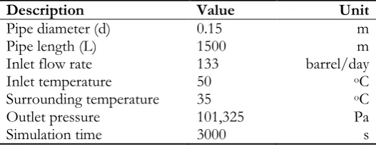
Table 2. Parameters for computational fluid dynamics simulation test.
Description Value Unit
Pipe diameter (d) 0.15 m Pipe length (L) 1500 m Inlet flow rate 133 barrel/day Inlet temperature 50 oC
Surrounding temperature 35 oC
[image:3.595.166.430.610.713.2]Fig. 1. The schematic diagram of the straight pipe model.
To study the effect of crude oil properties on the transport profile inside a pipeline, numerical simulation was tested under laminar unsteady state conditions. The Reynolds number of the flow in the pipeline was in the range of 35.63 to 261.16, depending on the condition. It is apparent that the Reynolds number is low for crude oil flow due to its high viscosity. The Peclet numbers were in the range of 15,999.00 to 22,752.29, and the Biot number was 1.83. Because the Peclet number was high, the convection was important. In addition, in this study, the Biot number implies that the conduction was much slower than the convection and temperature gradients dominant in the pipeline. A crude oil liquid flow was simulated with a 30,000 cell straight pipe model after grid independency testing. The simulation test operated until a steady state was reached. The details about the validation of this study used to develop the computer program code with literature experimental data can be found in Rukthong [15] and Rukthong et al. [16]. In this study, the result trends from the developed computational fluid dynamics simulation program were verified with the commercial program, ANSYS FLUENT [17], and theoretical transport phenomena concept.
2.3. Design of Experiments
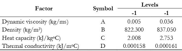
The first important step in the design of an experiment is the selection of suitable factors and their levels. In this study, four physical property factors (dynamic viscosity, density, heat capacity and thermal conductivity) were considered and compared in two levels as shown in Table 3. The two levels factorial experimental design methodology was used for screening the effect of each parameter [18]. With the 24
design, the low and high levels of factors are denoted by the code -1, 1, respectively. The parameters and their levels were selected based on the available literature and some experiments of QH crude oil [19] in the real operating temperature range. For the 24 factorial design, an orthogonal array is designed, and the
response numerical data is then obtained from a single replicate without experimental error. In this study, the location of wax appearance represented by pipe distance was used as the response, based on the wax appearance temperature (47oC) for QH crude oil. 16 runs were made in random order to avoid systematic
bias. The 24 factorial experimental design is shown in Table 4. The factorial design method has an
advantage to analyze the complex experiment systematically and to reduce the random error in the real experiment; however, the random error will not occur in the CFD simulation. On the other hand, a disadvantage or limitation of the factorial design method is the number of runs. Only two values, maximum and minimum, are considered with this method. However, the purpose of this study was only the screening process and to investigate the effect of the important parameters. Therefore, this issue did not impact the CFD simulation results.
Table 3. Physical property factors and their levels.
Factor Symbol Levels
-1 -1
Dynamic viscosity (kg/ms) A 0.005 0.036 Density (kg/m3) B 822.300 837.050
Heat capacity (kJ/kgoC) C 2.008 2.753
Thermal conductivity (kJ/moC) D 0.000158 0.000161
[image:4.595.148.445.82.166.2] [image:4.595.141.456.651.740.2]Table 4. 24 factorial experimental design based on code levels and their responses.
Run A B C D Distance
1 -1 1 -1 -1 221.4
2 -1 -1 1 1 297.9
3 -1 1 1 1 302.9
4 1 -1 1 -1 298.4
5 1 -1 -1 1 217.4
6 1 1 -1 -1 221.4
7 -1 1 -1 1 221.1
8 1 1 -1 1 221.1
9 -1 -1 -1 1 217.1
10 -1 1 1 -1 303.4
11 1 1 1 -1 303.4
12 1 -1 -1 -1 217.7
13 -1 -1 1 -1 297.9
14 1 1 1 1 303.4
15 -1 -1 -1 -1 217.4
16 1 -1 1 1 297.9
3.
Results and discussion
3.1. Numerical Result—Transport Profile in a Crude Oil Pipeline
According to the 24 factorial experimental design, 16 runs of simulation were carried out to obtain 16 flow
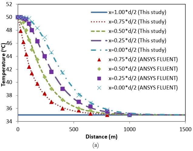
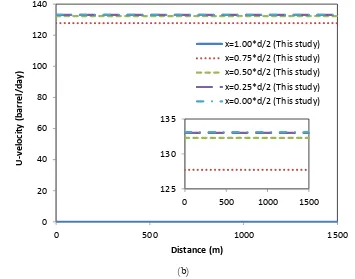
patterns represented by distribution profiles of crude oil flow in the pipeline. The results of the simulation showed that all 16 profiles had quite similar patterns. The examples of temperature and U-velocity profile line graphs are shown in Figs. 2(a) and 2(b), respectively. Each graph line in Fig. 2 shows the temperature and U-velocity at each position of the pipe diameter, respectively. In addition, Figs. 3(a) and 3(b) display the contour plot of corresponding temperature and U-velocity profiles, respectively.
(a)
34 36 38 40 42 44 46 48 50 52
0 500 1000 1500
Tem
p
e
ratu
re
(
oC)
Distance (m)
[image:5.595.140.458.478.726.2](b)
Fig. 2. Line graphs of (a) temperature and (b) U-velocity (barrel/day) of crude oil in the pipeline from the developed computational fluid dynamics simulation program (Each curve represents the various radial position of the pipe).
(a)
0 20 40 60 80 100 120 140
0 500 1000 1500
U
-v
e
lo
ci
ty
(b
ar
re
l/
d
ay
)
Distance (m)
x=1.00*d/2 (This study) x=0.75*d/2 (This study) x=0.50*d/2 (This study) x=0.25*d/2 (This study) x=0.00*d/2 (This study)
Temperature contour (oC)
Node number in y-direction (-)
N
o
d
e
n
u
m
b
e
r
in
x
-d
ir
e
c
ti
o
n
(
-)
500 1000 1500 2000 2500 3000
1 2 3 4 5 6 7 8 9 10
36 38 40 42 44 46 48 125
130 135
[image:6.595.114.469.85.364.2](b)
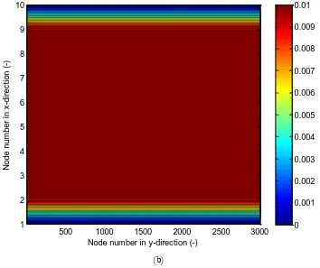
Fig. 3. Contour plots of (a) temperature and (b) U-velocity (m/s) of crude oil in the pipeline from the developed computational fluid dynamics simulation program.
In Fig. 2, each curve represents the results from various radial positions of the pipeline from the developed computational fluid dynamics code, and each square symbol shows the corresponding results from the commercial computational fluid dynamics program, ANSYS FLUENT.
The temperature of the crude oil in the pipe center had a maximum value and decreased along the radial direction of the pipe until it reached the pipe wall - the temperature of the pipe wall was the same as surrounding temperature. The difference between each profile was the decreasing rate of crude oil temperature which was affected by the surrounding environment. The crude oil near the pipe wall will transfer internal energy to the environment before the crude oil at the pipe center. The velocity, or flow rate, of the crude oil in the pipeline was quite constant. The decrease of crude oil temperature near the pipe wall led to a rapid increase in the oil viscosity near the wall, which made the crude oil velocity drop slightly along the pipe radial direction as can be seen in the velocity contour plot in Fig. 3(b). These results are in agreement with the previously reported trends by Rukthong [15] and Rukthong et al. [16].
As regards the obtained results along the pipeline length, the crude oil temperature decreased along the pipe distance due to heat loss to the surrounding. The higher temperature difference is the more driving force of this obtained phenomenon. The crude oil U-velocities were constant throughout the pipeline distance with parabola profile at each pipeline position because of constant cross-sectional area of the pipeline (Fig. 2(b)). The parabola velocity profile is a conventional velocity profile with laminar flow operating characteristics.
Comparison between temperature gradient profiles in the crude oil pipeline obtained from the developed computational fluid dynamics simulation program [17], ANSYS FLUENT, and the theoretical transport phenomena concept [20] after the system reached the steady state found that the obtained temperature and U-velocity gradient profile trends were quite similar. Therefore, the model accuracy was validated. As stated above, the detail comparison results were previously presented in Rukthong [15] and Rukthong et al. [16].
Node number in y-direction (-)
N
o
d
e
n
u
m
b
e
r
in
x
-d
ir
e
c
ti
o
n
(
-)
500 1000 1500 2000 2500 3000
1 2 3 4 5 6 7 8 9 10
[image:7.595.122.476.78.375.2]The results of all 16 responses with a single replicate are shown in Table 4. ANOVA was used to analyze the result of the simulation. The statistical analysis of the results obtained with a confidence level of 95%, or p-value equal to 0.05, is shown in Table 5. When considering the p-value, B and C factors had a statistically significant effect at 95% confidence level. It was found from the higher F-value that the heat capacity of crude oil had a more significant effect than the density of crude oil. The residual error term combines the effect of uncontrollable factors, thus excluding it from the analysis results [21, 22]. The obtained mathematic model is:
1
0.0626 0.000274065*B 0.00492569 *C
y (2)
where y is the location of wax appearance represented by pipe distance, and B and C are the actual values of crude oil density and crude oil heat capacity, respectively.
Table 5. Analysis of Variance (ANOVA).
Source Sum of Squares Degree of freedom
(DF)
Mean
Square F-value P-value
Model 0.000389401 2 1.95E-04 141789.4 < 0.0001 B 1.20179E-06 1 1.2E-06 875.1939 < 0.0001 C 0.000388199 1 3.88E-04 282703.5 < 0.0001 Residual 1.78512E-08 13 1.37E-09
Total 0.000389418 15
3.3. The Effect of Density and Heat Capacity on Pipe Distance or Location of Wax Appearance
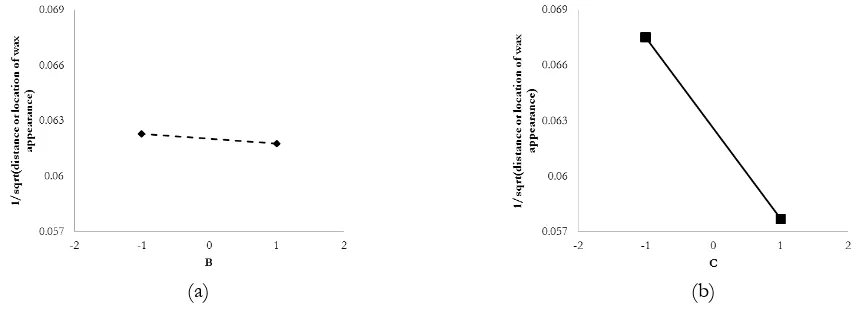
As mentioned previously, crude oil heat capacity was a more significant factor on pipe distance or location of wax appearance than crude oil density, as can be observed in Fig. 4. Both factors had a negative effect on the reciprocal of square root of pipe distance or location of wax appearance or had a positive effect on pipe distance or location of wax appearance. The location of wax appearance increased dramatically as the crude oil heat capacity increased, whereas the location of wax appearance slightly increased as the crude oil density increased.
(a) (b)
Fig. 4. Main factor effects: (a) density and (b) heat capacity of crude oil.
[image:8.595.88.506.311.412.2] [image:8.595.85.519.538.702.2]as heat capacity increases [8], resulting in a slower waxing time. The pipe distance or location of wax appearance then increases.
Density is defined as mass divided by volume, which is a specific property of matter dependent on the temperature of matter. Consider the heat transfer equation:
Qmc T (3)
where m is mass of crude oil, c is heat capacity and T is the change in temperature. When m is replaced by density and volume, the quantity of heat, or heat rate, required to change the temperature increases with an increase in density, causing slower waxing time. As a consequence, the pipe distance or location of wax appearance increases. When density of crude oil increases, it also causes the decrease in crude oil velocity because it needs more driving force to transfer bulk of crude oil along the pipeline distance [25].
4.
Conclusions
The aim of this study was to investigate the effect of crude oil properties (dynamic viscosity, density, heat capacity and thermal conductivity) on the transport profile of crude oil by developing an in-house computational fluid dynamics model. The viscous liquid phase flow was successfully simulated in a straight pipeline model. The 16 simulation runs were carried out based on the 24 factorial experimental design. It
was found that all 16 flow distribution trends obtained from the developed computational fluid dynamics simulation program were quite similar. The crude oil temperature decreased along the pipe distance due to heat loss to the surrounding environment. Besides, the temperature of the oil in the pipe center had a maximum value and decreased along the radial direction of the pipe until it reached the pipe wall. The velocity, or flow rate, of the crude oil in the pipeline was quite constant along the pipeline with parabola profile at each pipeline position.
The influence of various physical properties on the transport profile was analyzed using the 24 factorial
experimental design. The result showed that crude oil heat capacity and density had statistical significance at 95% confidence level. The heat capacity had the most significant effect on wax appearance. The obtained mathematical equations presented a reliable result with high R-squared value. Both factors had a positive effect on pipe distance or location of wax appearance. To apply this knowledge in the other real situation, the physical properties of crude oil should be adjusted by mixing it with some lighter/heavier crude oil or other chemical compositions/solvents [15, 26] to prevent the occurrence of wax inside the transportation pipeline.
Acknowledgements
The authors wish to gratefully acknowledge a Scholarship from the Graduate School, Chulalongkorn University to commemorate the 72nd Anniversary of the Birth of His Majesty King Bhumibala Aduladeja and a CU Graduate School Thesis Grant as well as a Grant from the Thailand Research Fund (IRG5780001/TRG5780205), PETROMAT and PTT Public Company Limited for financial support of this study.
References
[1] B. Yu, C. Li, Z. Zhang, X. Liu, J. Zhang, J. Wei, S. Sun, and J. Huang, “Numerical simulation of a buried hot crude oil pipeline under normal operation,” Appl. Therm. Eng., vol. 30, no, 17, pp. 2670– 2679, 2010.
[2] S. Kelesoglu, B. H. Pettersen, and J. Sjöblom, “Flow properties of water-in-North Sea heavy crude oil emulsions,” J. Pet. Sci. Eng., vol. 100, pp. 14–23, 2012.
[3] L. D. Stasiuk and L.R. Snowdon, “Fluorescence micro-spectrometry of synthetic and natural hydrocarbon fluid inclusions: Crude oil chemistry, density and application to petroleum migration,”
Appl. Geochem., vol. 12, no. 3, pp. 229–241, 1997.
hydrocarbon production system,” J. Pet. Sci. Eng., vol. 108, pp. 128–136, 2013.
[6] A. Ahmadpour, K. Sadeghy, and S.-R. Maddah-Sadatieh, “The effect of a variable plastic viscosity on the restart problem of pipelines filled with gelled waxy crude oils,” J. Non-Newton. Fluid, vol. 205, pp. 16–27, 2014.
[7] A. N. El-hoshoudy, A. B. Farag, O. I. M. Ali, M. H. EL-Batanoney, S. E. M. Desouky, and M. Ramzi, “New correlations for prediction of viscosity and density of Egyptian oil,” Fuel, vol. 112, pp. 277–282, 2013.
[8] H. K. Verstreeg, and W. Malalasekera, An Introduction to Computational Fluid Dynamics: The Finite Volume Method, 2nd ed. London, England: Longman, 2007.
[9] X. Xing, D. Dou, Y. Li, and C. Wu, “Optimizing control parameters for crude pipeline preheating through numerical simulation,” Appl. Therm. Eng., vol. 51, no. 1–2, pp. 890–898, 2013.
[10] L. Kumar, K. Paso, and J. Sjöblomm “Numerical study of flow restart in the pipeline filled with weakly compressible waxy crude oil in non-isothermal condition,” J. Non-Newton. Fluid, vol. 223, pp. 9–19, 2015.
[11] H. Zhu, X. Yang, J. Li, and N. Li, “Simulation analysis of thermal influential factors on crude oil temperature when double pipelines are laid in one ditch,” Adv. Eng. Softw., vol. 65, pp. 23–31, 2013. [12] B. Yu, Y. Wang, J. Zhang, X. Liu, Z. Zhang, and K. Wang, “Thermal impact of the products pipeline
on the crude oil pipeline laid in one ditch—The effect of pipeline interval,” Int. J. Heat Mass Transfer, vol. 51, no. 3–4, pp. 597–609, 2008.
[13] Z. Huang, M. Senra, R. Kapoor, and H.S. Fogler, “Wax deposition modeling of oil/water stratified channel flow,” AIChE J., vol. 57, no. 4, pp. 841–851, 2011.
[14] N. H. Abdurahman, Y. M. Rosli, N. H. Azhari, and B. A. Hayder, “Pipeline transportation of viscous crudes as concentrated oil-in-water emulsions,” J. Pet. Sci. Eng., vol. 90–91, pp. 139–144, 2012. [15] W. Rukthong, “Development of computational fluid dynamics program for flow inside crude oil
pipeline,” M.S. thesis, Department of Chemical Technology, Faculty of Science, Chulalongkorn University, Bangkok, Thailand, 2014.
[16] W. Rukthong, W. Weerapakkaroon, U. Wongsiriwan, P. Piumsomboon, and B. Chalermsinsuwan, “Integration of computational fluid dynamics simulation and statistical factorial experimental design of thick-wall crude oil pipeline with heat loss,” Adv. Eng. Softw., vol. 86, pp. 49–54, 2015.
[17] ANSYS FLUENT Inc., ANSYS Fluent 12.0 User’s Guide, 1st ed. Lebanon, United States: ANSY Fluent Inc., 2006.
[18] D. C. Montgomery, Design and Analysis of Experiments. 5th ed. New York, United States: John Wiley and Sons, 2001.
[19] Z. Guozhong and L. Gang, “Study on the wax deposition of waxy crude in pipelines and its application,” J. Pet. Sci. Eng., vol. 70, no. 1–2, pp. 1–9, 2010.
[20] R. B. Bird, W. E. Stewart, and E. N. Lightfoot, Transport Phenomena. New York, United States: John Wiley and Sons, 2002.
[21] L. A. Kareem, T. M. Iwalewa, and J. E. Omeke, “Isobaric specific heat capacity of natural gas as a function of specific gravity, pressure and temperature,” J. Nat. Gas Sci. Eng., vol. 19, pp. 74–83, 2014. [22] W. Rukthong, T. Phattharanid, S. Sunphorka, P. Piumsomboon, and B. Chalermsinsuwan,
“Computation of biomass combustion characteristic and kinetic parameters by using thermogravimetric analysis,” Engineering Journal, vol. 19, no. 2, pp. 41-57, 2015.
[23] F. P. Incropera and D. P. DeWitt, Introduction to Heat Transfer, 4th ed. New York, United States: John Wiley & Sons, 2001.
[24] L. Bai, Y. Jiang, D. Huang, and X. Liu, “A novel scheduling strategy for crude oil blending,” Chin. J. Chem. Eng., vol. 18, no. 5, pp. 777–786, 2010.
[25] N. Ghasem and R. Henda, Principles of Chemical Engineering Processes: Material and Energy Balances, 2nd ed. Boca Raton, United States: CRC Press, 2014.
![Table 1. Physical properties of some Malaysian oilfields [7].](https://thumb-us.123doks.com/thumbv2/123dok_us/8109111.235863/2.595.64.535.340.430/table-physical-properties-malaysian-oilfields.webp)