Neural correlates of economic and moral decision making

AND MORAL DECISION-MAKING

Thesis by Cédric Robert Anen

In Partial Fulfillment of the Requirements for the degree of

Doctor of Philosophy

CALIFORNIA INSTITUTE OF TECHNOLOGY

Pasadena, California 2007

© 2007

ACKNOWLEDGEMENTS

Having constantly worked in electrical engineering, my encounter with neuroeconomics was rather a coincidence. After having spent the first year of my Ph.D. taking classes in electrical engineering at Caltech, in summer 2002 I came across a newspaper article about the inconsistencies in choices when rewards are presented at different points in time, a phenomenon known as time discounting in behavioral economics. Researchers were trying to uncover the neural correlates of evaluating future rewards, and my interest was immediately sparked. How great would it be if we could look into people’s brains and analyze and explain the greatest mysteries of human behavior?! Although neuroeconomics was at that time a brand new science, I was extremely happy to find out that several professors at Caltech were already working in that field, and I was able to join Steve Quartz’s lab in fall 2002.

I have spent wonderful years at Caltech, both on a personal and intellectual level. In my eyes no other place provides a better research environment to students and faculty. The reason is twofold: first of all, the relatively small size of Caltech allows different departments to work closely together. A lot of faculty have positions in two or more departments, and the students in their research groups also have diversified backgrounds. I believe that the research sparked by those interdisciplinary collaborations is at the core of scientific success. Secondly, no other campus has a concentration of such talented professors and students. Everyone at Caltech is bright and alert, and it seems that no-one ever gets tired of having discussion about research.

Camerer, Read Montague (Baylor College of Medicine), and John O’Doherty. I would also like to thank the electrical engineering professors on my thesis committee, Shuki Bruck, Robert McEliece, and PP Vaidyanathan, for supporting me in my choice to pursue research that is not so typical for an electrical engineer.

A big thank you goes out to all the wonderful people at Caltech that I have worked with, discussed scientific problems with or just had fun with, in particular Ulrik Beierholm, Meghana Bhatt, Tony Bruguier, Ilja Friedel, Alan Hampton, Vanessa Heckman, Ming Hsu, Shreesh Mysore and Kerstin Preuschoff. All of you have made my time at Caltech special and it is with great regret that I will have to leave you.

Apart from science, my other love is fencing, and the Caltech Fencing Team has served as an important balance in my life. It was great hanging out and fencing with all of you, and in particular my friends and teammates: George, Yann, Joe, Randy, Christine, Rebecca, Kathy, Ken, Haomiao, Laura, and Steve. Caltech also offered me an immense opportunity by being able to coach the Caltech fencing team in 2004-5 and 2005-6, and to be the head coach of the team in 2006-7. This allowed me to experience the joy of teaching and to share my love of fencing with other people.

ABSTRACT

Our daily lives are shaped by a series of decision processes, ranging from very unimportant choices to life-changing judgments. The complexity of the decision processes increases tremendously when the decision-making takes place in a social context, i.e., when other human beings are directly involved in the decision. In such conditions the decision-maker not only tries to maximize his own utility, but also needs to take into account the interdependent nature of the situation. Information about others’ preferences, characteristics, and actions play an important role, and need to be thoroughly evaluated and predicted before making a decision. In this thesis we explore the neural correlates of two different types of social decision-making.

In the first experiment I investigate economic decision-making in the context of a two-player social exchange game. In order to maximize their overall and personal earnings, players need to cooperate and build up a trust relationship with their partner. Synchronized neural data is recorded from the two interacting brains using functional magnetic resonance imaging. In this thesis I present four main findings: (i) the neural correlates of strategic uncertainty and how it can be used to predict a player’s future strategic choice; (ii) the dynamic interaction of the brains of two interacting players; (iii) the neural correlates of trust and its development over the course of the game; and (iv) how the brain distinguishes between one’s own actions and those of another person.

The second experiment investigates the neural basis of moral decision-making and other- regarding preferences. Subjects have to make a morally difficult decision between helping two groups of children while trading off between efficiency and equity. By parametrically varying these variables, I show how two brain structures, the insula and the caudate, are actively involved in the decision-making process.

TABLE OF CONTENTS

Acknowledgements ...iii

Abstract ... v

Table of Contents...vi

List of Illustrations and Tables ...viii

Chapter I: Introduction ... 1

I.1. Neuroeconomics... 2

I.2. Experiments in Neuroeconomics... 6

Chapter II: Basics of fMRI ... 9

II.1. MRI Physics... 9

II.2. Measuring the BOLD Signal... 13

II.3. fMRI Data Acquisition ... 15

II.4. fMRI Data Preprocessing ... 17

II.5. fMRI Data Analysis... 21

Chapter III: Neural Correlates of Economic Decision-Making ... 27

III.1. Background... 27

III.1.1. Behavioral Game Theory... 27

III.1.2. The Trust Game... 31

III.1.3. Previous Studies ... 34

III.2. Experimental Design and Methods... 35

III.2.1. Task ... 35

III.2.2. Subjects... 36

III.2.3. Experimental Setup ... 36

III.2.4. fMRI Data Acquisition and Preprocessing... 37

III.3. Behavioral Results... 39

III.4. Strategic Uncertainty and Prediction Analysis... 42

III.4.1. Background ... 42

III.4.2. GLM Analysis: New vs. Known Information... 45

III.4.3. ROI Analysis: Correlation between Later Decisions and Hrf . 47 III.4.4. Signal Magnitude Encodes Strategic Uncertainty... 50

III.4.5. Signal Magnitude Predicts Future Strategic Choice ... 51

III.4.6. Discriminant Analysis of Predictive Accuracy ... 53

III.4.7. Discussion and Conclusion... 54

III.4.8. Methods ... 58

III.5. Dynamic Cross-Brain Analysis... 62

III.5.1. Background ... 62

III.5.2. Dependency Measures ... 63

III.5.4. Results ... 70

III.5.5. Discussion and Conclusion... 76

III.6. Trust & Reciprocity... 80

III.6.1. Background ... 80

III.6.2. Reciprocity Predicts Trust... 81

III.6.3. “Intention to Trust” Signals ... 83

III.6.4. Model Building of Partner: Cross-Brain Analysis ... 83

III.6.5. Discussion and Conclusion... 87

III.6.6. Methods ... 90

III.7. Agency Attribution... 91

III.7.1. Background ... 91

III.7.2. Cross-Cingulate PCA Analysis... 93

III.7.3. Differential “Own” and “Other” Responses... 94

III.7.4. Agent-Specific Responses Disappear in Control Experiments 97 III.7.5. Cingulate Pattern Remains Constant for Several Variables .... 98

III.7.6. Discussion and Conclusion... 100

III.8. Conclusions ... 103

Chapter IV: Neural Correlates of Moral Decision-Making... 104

IV.1. Background ... 104

IV.2. Experimental Design and Methods ... 110

IV.2.1. Task ... 110

IV.2.2. Subjects ... 111

IV.2.3. Experimental Setup... 111

IV.2.4. fMRI Data Acquisition and Analysis ... 114

IV.3. Behavioral Measures and Behavioral Results... 115

IV.3.1. The Gini Coefficient ... 115

IV.3.2. Measures of Efficiency, Equity, and Utility... 117

IV.3.3. Behavioral Data ... 118

IV.3.4. Act/Omit Differences ... 120

IV.3.5. Inequity Aversion Models ... 121

IV.4. fMRI Results ... 124

IV.4.1. Difference Between Allocations... 124

IV.4.2. Correlates of Efficiency, Equity, and Utility in Take Trials.. 126

IV.4.3. Correlates of Efficiency, Equity, and Utility in Give Trials.. 127

IV.5. Discussion and Conclusions ... 129

IV.5.1. Insula Activations ... 130

IV.5.2. Caudate Activations... 132

IV.5.3. Conclusions... 133

IV.6. Methods ... 134

Chapter V: Conclusions... 136

LIST OF ILLUSTRATIONS AND TABLES

Figures Page

1. Available Choices in the Ellsberg Paradox ... 3

2. Spatiotemporal Resolution of Brain Recording Techniques ... 7

3. Hydrogen Nuclei in a Magnetic Field ... 10

4. Effect of A RF Pulse on the Net Magnetization... 11

5. T1-Weighted High-Resolution Anatomical MR Image... 13

6. * 2 T -Weighted Functional MR Image... 14

7. Shape of the Hemodynamic Response Function... 15

8. Full-Body Human 3-T MRI Scanner at Caltech ... 16

9. Normalization Procedure ... 19

10.Spatial Smoothing Procedure... 20

11.Sample Time-Series of a Voxel Within the Brain... 21

12.Effect of the Convolution with an Hrf... 23

13.fMRI Activations in Glass-Brain and on SPM Map ... 24

14.The Ultimatum Game... 27

15.The Prisoner’s Dilemma ... 28

16.The Public Goods Game ... 29

17.The Trust Game... 30

18.Fairness in the Trust Game ... 32

19.Hardware Setup of the Trust Game ... 35

20.Timeline of 1 Round of the Trust Game ... 37

21.Example #1 of Monetary Exchange ... 38

22.Example #2 of Monetary Exchange ... 39

23.Example #3 of Monetary Exchange ... 39

24.Average Investment and Repayment Ratios ... 40

25.Activations in the Trustee Brain ... 45

27.Time-Courses Predict Strategic Choice... 48

28.Analysis of Signal Magnitudes ... 51

29.Performance of the Prediction Analysis ... 53

30.Activations in the Investor Brain ... 58

31.Distribution of the Mutual Information ... 67

32.Activations in the Investor Brain ... 70

33.Activations in the Trustee Brain ... 70

34.Game Dynamics ... 72

35.Cross-Round Dynamics in BA9 ... 73

36.Cross-Round Dynamics in Primary Visual Cortex ... 76

37.Correlates of Reciprocity in a Multi-Round Economic Exchange ... 81

38.Correlograms of the “Intention to Trust” ... 84

39.Neural Correlates of Reputation Building in the Trustee Brain ... 85

40.Model Building in the Trustee Brain... 86

41.Cingulate Segmentation ... 93

42.Cross-Cingulate Correlations... 94

43.Agent-Specific Responses... 95

44.Cingulate Pattern of “Me” and “Not Me” ... 98

45.Classical Dilemmas in Moral Decision-Making ... 105

46.Activations in Personal Moral Dilemmas ... 107

47.Example of a Child’s Biography ... 111

48.Timeline of the Moral Decision-Making Task... 112

49.Graphical Representation of the Gini Coefficient... 114

50.Wealth Distribution in the World ... 115

51.Subject Behavior in the Moral Task ... 118

52.Act/Omit Differences in the Moral Task... 120

53.Coefficients in the Inequity Aversion Model ... 121

54.Repartition of α_TakeAcross Age... 122

55.Difference Between Allocations... 123

57.Delta Equity in Take Trials... 125

58.Delta Utility in Take Trials ... 126

59.Delta Equity in Give Trials ... 127

60.Delta Efficiency in Give Trials ... 128

61.Interpretation of Delta Equity ... 130

Tables Page 1. Investment > Repayment Regions for the Trustee... 44

2. Repayment > Investment Regions for the Investor... 58

3. Summary of Activations at the Revelation Screens... 71

4. Summary of Game Dynamics... 74

5. Allocation of Meals... 110

6. Activations in the Insula for |ΔM|... 123

7. Activations in the Insula for ΔG During Take Trials... 125

C h a p t e r 1

INTRODUCTION

All living organisms face situations that require evaluating various alternatives and making decisions that are often critical to their survival. For example, a hunting tiger in the grasslands needs to decide whether it is sufficiently close to its prey to attack, or whether it should try to sneak closer at the risk of being seen. Such choices are typically associated with factors such as risk, uncertainty, reward, or punishment, which need to be estimated in order to make the best possible decision. As most organisms learn through experience, their decision-making processes are continuously updated and optimized, and eventually lead (after enough exposure or training) to a set of rules and actions that define the organism’s behavior.

I.1. Neuroeconomics

Human decision-making and choice theory have been thoroughly investigated in a variety of fields. Cognitive psychologists attempt to describe and understand behavior and mental processes by recording behavioral variables and psychometric measurements in controlled laboratory experiments. Behavioral economists aim to understand how human and social cognitive and emotional biases affect economic decisions, and they do this by designing a whole set of experiments and creating models to predict human choice. Cognitive neuroscientists are concerned with the neural substrates of mental processes and their behavioral manifestations. Traditionally, collaborations between these closely related fields have been relatively limited, but the recent break-through in neuroscientific technologies has given rise to a new interdisciplinary science that synthesizes the fields: neuroeconomics.

Neuroeconomics seeks to identify and understand the neural processes that underlie human decision-making by studying how the brain interacts with its environment to produce economic behavior. As such neuroeconomics is a crossroads between economics, psychology, and neuroscience that aims to better understand choice theory by unifying the separate approaches. In neuroeconomics theories and models are constrained by facts and by biological processes that determine how the brain functions. If a certain economic theory seems to describe choice behavior very accurately, but there is no evidence that the brain uses that model (for example due to limited computational power), then that theory can be discarded as a model of human behavior. Hence neuroeconomics tries more than just to describe choice behavior—it seeks to understand how decision-making works on the neural and cognitive levels.

The insights that neuroeconomics can provide are best illustrated by an example: the Ellsberg paradox (Keynes 1921; Ellsberg 1961). Imagine 2 urns containing 100 balls each. Urn A (risky urn) contains exactly 50 black and 50 red balls, and Urn B (ambiguous urn) contains 100 black or red balls, the exact composition of which is unknown (Fig. 1). The balls are well mixed so that each ball is equally likely to be drawn. A bet on any color gives a payoff of $20 if a ball of the chosen color is drawn, and $0 otherwise.

Fig. 1: Available choices in the Ellsberg paradox

In a situation like this most people prefer drawing a ball from Urn A rather that Urn B independently of the color, preferring known probabilities over unknown probabilities. If preferences are strictly based on probabilities, this pattern is a paradox leading to a violation of standard decision theory. Indeed, preferring a bet on a red ball from Urn A over Urn B implies thatp_risk(red)> p_am(red). Similarly, preferring a bet on a blue ball from Urn A over Urn B implies thatp_risk(blue)> p_amb(blue). By adding together those two inequalities and taking into account the fact that the probabilities of red and blue must add up to 1, this leads to a contradiction:

4 4 4 4 3 4 4 4 4 2 1 4 4 4 4 3 4 4 4 4 2 1 1 1 ) ( ) ( ) ( ) ( = = + >

+ p blue p red p blue

red

p_{risk risk amb amb}

This paradox can be resolved if one allows for subjective probabilities wherep_amb(red)+p_amb(blue)<1, e.g. p_amb(red)= p_amb(blue)=0.45, the remaining 0.1 representing the amount of uncertainty that is associated with the ambiguous gamble. Although this trick solves the paradox mathematically, it does not explain how the brain makes a decision. Recently neuroeconomists investigated this paradox (Hsu, Bhatt et al. 2005; Huettel, Stowe et al. 2006), and found that different brain mechanisms are recruited to process risk and ambiguity. More specifically, they found that the amygdala and the lateral orbitofrontal cortex are more activated when facing ambiguous choices whereas the dorsal striatum is more activated in risky decision-making. They proposed a neural circuitry that responds to various degrees of uncertainty, in contrast to classical decision theory that makes no distinction between ambiguity and risk.

By investigating classical concepts and theories from behavioral economics (such as the Ellsberg paradox) and through the use of neuroscientific tools in combination with neuroscientific expertise, neuroeconomists try to create a mathematically and biologically plausible model of human behavior. Despite being a relatively new science, neuroeconomics has already significantly contributed to knowledge in a variety of areas. But it has also drawn some criticism, most notably from Gul and Pesendorfer who argue that neuroscience addresses different questions, and can therefore not provide any insight into economic theories (Gul and Pesendorfer 2005).

“Neuroscience evidence cannot refute economic models because the latter make no assumptions

and draw no conclusions about the physiology of the brain. Conversely, brain science cannot

revolutionize economics because the latter has no vehicle for addressing the concerns of

economics.”

as it focuses on what provides the most hedonic utility to subjects rather than the economic data itself:

“What makes individuals happy (‘true utility’) differs from what they choose. Economic

welfare analysis should use true utility rather than the utilities governing choice (‘choice

utility’).”

A lot of the criticism is also targeted towards neuromarketing, a closely related field that studies consumers’ brain responses to marketing stimuli (e.g., brand names, price, design) in order to provide better products and more efficient marketing campaigns. Most of that criticism comes from the popular press as well as from consumer protection agencies that are afraid that neuroeconomics and neuromarketing could be used to manipulate consumers’ choices. This is however far from the current standing of things as neuroeconomists are currently just trying to understand consumers’ choices.

Yet many behavioral economists, psychologists, and neuroscientists view neuroeconomics as a means to better understand how neural activity gives rise to a cognitive capacity for economic decision-making. Vernon Smith, 2002 Nobel Laureate in Economics, best expresses this optimistic attitude in his Nobel lecture "Constructivist and Ecological Rationality in Economics."

"New brain imaging technologies have motivated neuroeconomic studies of the internal order

of the mind and its links with the spectrum of human decisions ... its promise suggests a

I.2. Experiments in Neuroeconomics

Neuroeconomics draws from related fields by using their tools and concepts in order to understand choice behavior. While behavioral economics and cognitive psychology provide the conceptual and mathematical frameworks as well as the experimental designs, neuroscience provides the scientific tools to study the neural correlates of choice behavior. Neuroeconomics extends the approach used in behavioral economics by recording neural data (and also often psychophysiologic data such as heart beat or skin conductance) in addition to behavioral data. In a typical behavioral economic experiment subjects are asked to choose between different options: for example, different gambles. By varying the experiment’s parameters over a whole range of values (e.g., gambles with different stakes), economists create a model that predicts subjects’ choices. Neuroeconomists check the biological validity of that model and try to improve its accuracy by making use of the neural data.

Experiments can range from very simple choice tasks to more sophisticated paradigms where subjects have to figure out non-trivial problems. Neuroeconomists are also interested in how people make choices with respect to others, and thus they conduct multi-subject experiments with the neural responses of one or more subjects being recorded simultaneously. The incentive for a subject is always to maximize the amount of money he can earn. Most experiments in neuroeconomics have been thoroughly studied by behavioral psychologists and/or economists (e.g., in game theory), which allows them to test the validity of existing models on neural data.

Functional magnetic resonance imaging (fMRI) is the most commonly used method in neuroeconomics as it provides a great tradeoff between temporal and spatial resolution (down to 1–2 mm2 and 0.5 sec). Furthermore it is non-invasive and does not require any tagging of the blood with radioisotopes (as does PET, for example). One of its drawbacks is that fMRI is only an indirect measure of brain activity (see Chapter 2 for more details). Better spatial and temporal resolutions are provided by electrophysiological measures such as single unit recordings or patch clamp techniques which record brain activity directly from neurons. However, because of its invasive nature, it is only used on animals.

Fig. 2: Spatiotemporal resolution of brain recording techniques (from Jezzard et al., 2001). MEG = Magneto-EncephaloGraphy, ERP = Evoked Response Potentials, fMRI = functional Magnetic Resonance Imaging, PET = Positron Emission Tomography

C h a p t e r 2

BASICS OF FMRI

The results presented in this thesis have been obtained using functional magnetic resonance imaging (fMRI). In this chapter I will discuss how fMRI works and how fMRI data analysis is done. This chapter intends in no way to be complete, but only serves as an outline to describe the basic principles of fMRI required to understand the neuronal data analysis from neuroeconomic experiments. For a detailed review of fMRI methods see Jezzard or Huettel (Jezzard 2001; Huettel, Song et al. 2004).

II.1. MRI Physics

Fig. 3: Hydrogen nuclei in a magnetic field

When one applies a brief magnetic field orthogonal toBr₀ (called a 90 degree excitatory radio frequency or RF pulse), the aligned spins tip over to the transverse field. When the orthogonal magnetic field is removed, the spins do not immediately realign back withBr₀, but they precess around Br₀at a frequency directly proportional to it (Fig. 4) according to:

0

0 γB

ω =

where ω₀ is the precessing frequency (also called Larmor frequency) and γ is the gyromagnetic ratio. This precession gives rise to a longitudinal magnetization M_land a transverse magnetization M_t. As the spins gradually align back withBr₀, the longitudinal magnetization grows back to M₀, whereas the transverse magnetization decreases to 0. The times that it takes for these events to occur are known as the relaxation times

1

Fig. 4: Effect of a RF pulse on the net magnetization. 1. Net magnetization M0 under the influence of a magnetic field B0. 2. A 90

degree RF pulse is applied, and tips the net magnetization over to the transverse field. 3. When the RF pulse is removed, the spins precess around B0, creating a net magnetization vector M _{that rotates}

around z, and gradually regains its original intensity M0. M can be

decomposed into a longitudinal magnetization Ml and a transverse

The time course where M grows back to M₀ in the longitudinal direction is mathematically described by an exponential curve:

) 1

( /1

0

T t

l M e

M = − −

where t is time and T₁ depends on the nature of the tissue. The time it takes for the transverse magnetization to completely disappear is much shorter thanT₁. This is caused by small fluctuations in the precessing speed of the spins that cause them to gradually fall out of phase. T₂ is thus solely caused by spin-spin interactions and is independent of the nature of the tissue. This time course of such a relaxation is also described by an exponential curve:

2

/ 0

T t t M e

M = −

In reality this decay is actually much faster, because in addition to the spins interacting with each other, they are also affected by small inconsistencies in the applied magnetic field B₀. When objects are placed in a magnetic field, they become magnetized themselves and changes in local magnetic susceptibility create distortions in the magnetic field. This results in a much faster decay of the transverse magnetization with a time constant *

2

T , which is dependent on the nature of the tissue.

1

Fig. 5: T1-weighted high-resolution anatomical MR image. From left to right: coronal view, sagittal view, axial view

II.2. Measuring the BOLD Signal

1

T -weighted images allow us to discern between different tissues in the brain, but cannot provide any information about whether or not a brain structure is active during a certain task. This is achieved by using the fact that an increase/decrease in blood flow and blood oxygenation (known as hemodynamics) is a result of increased/decreased neuronal activity: firing neurons consume more of the oxygen that is being carried by hemoglobin in red blood cells than non-firing neurons consume. Oxygenated hemoglobin is diamagnetic and has the same magnetic properties as the rest of the tissue, whereas deoxygenated hemoglobin is paramagnetic. Deoxygenated hemoglobin causes a change in the magnetic susceptibility of the local blood supply, thereby causing an inhomogeneity in the local magnetic field, which in turn decreases the time constant *

2

T . This effect was first discovered by Ogawa (Ogawa, Lee et al. 1990), who showed that when mice breathed different concentrations of oxygen, the low concentration oxygen caused a significant signal drop in blood vessels in the brain. By measuring the time constant *

2

T , one can thus obtain Blood Oxygenation Level Dependent (BOLD) images which are the type of images that are acquired by fMRI imaging (Fig. 6). In *

2

grey and grey matter appears white, but the more interesting fact is that intensity changes as a function of brain activity.

Fig. 6: T₂*-weighted functional MR image. From left to right: coronal view, sagittal view, axial view

Although the connection between changes in blood flow and changes in neural activity has been known for a long time (Roy and Sherrington 1890), the exact cause of this relationship is still unclear. It has been argued that the increased blood flow fills the demand of oxygen and glucose needed for the restoration of energy supply during neuronal activity. This is consistent with the fact that the BOLD signal correlates most strongly with measures of presynaptic activity as shown by Logothetis (Logothetis, Pauls et al. 2001). Heeger has also shown that fMRI responses in the monkey medial temporal lobe correlate with single neuron firing rates (Heeger, Huk et al. 2000), and recently Logothetis’s group has shown that negative fMRI responses correlate with decreases in neuronal activity in the monkey visual area V1 (Shmuel, Augath et al. 2006). Although these studies and other ones do not explain the reason for the relation between blood flow and neuronal firing, they do provide good evidence to use fMRI as a measure of neuronal activity.

temporal limitation, in combination with the low spatial resolution, makes it impossible to record from individual neurons, but measures the activity of rather large sets of neurons.

Fig. 7: Shape of the hemodynamic response function. Initial dip not shown here

II.3. fMRI Data Acquisition

another gradient is applied that causes the spins to be out of phase with respect to each other in a predictable manner along the y-axis. Both the frequency and phase encoding are then recovered through Fourier transform to recover the signal from a single voxel.

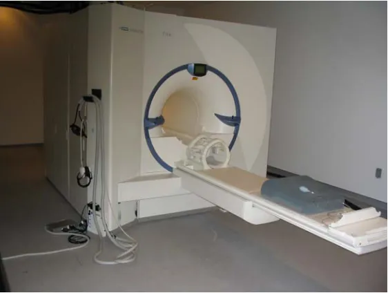
Fig. 8: Full-body human 3-T MRI scanner at Caltech

In a typical fMRI experiment subjects lie on their back in a MRI scanner (Fig. 8) with their head constrained by pads to avoid motion artifacts. They wear goggles that allow them to view a projected computer screen, and they hold response boxes in their hands to make choices during the experiment. Experiments last anywhere form 20 minutes to 2 hours, during which 3 sets of images are acquired: 1. a low resolution localizer that shows where the subject’s head is positioned, 2. a high-resolution 3-D anatomical image that gives a detailed view of the structure of the brain (also called anatomical T₁ image), and 3. an fMRI image set that is composed of a series of 3-D pictures taken every 1–2 seconds (also called fMRI time-series).

important noise sources are thermal noise from the scanner, scanner drift, subject head motion, inhomogeneities in the magnetic field resulting from different magnetic susceptibility (e.g., the nasal cavity), physiological artifacts (e.g., respiratory cycle) and anatomical differences between subjects. Some of these sources of noise can be compensated for through optimizing scanning parameters and by image preprocessing, but the most powerful method is to repeat all stimuli over many trials and many subjects to allow for a statistical analysis. In the next two parts I will describe how the functional time-series and the anatomical image will be combined into a statistical activation map of the brain.

II.4. fMRI Data Preprocessing

The purpose of the preprocessing is twofold: it removes some of the introduced noise, and it prepares the fMRI images for a statistical analysis. There are five steps that need to be performed in the order listed below. All fMRI data preprocessing in this thesis was done using the statistical package SPM2 (Wellcome Department of Cognitive Neurology, London, UK, http://www.fil.ion.ucl.ac.uk/spm/software/spm2).

Slice Time Correction

Realignment

One of major sources of noise in fMRI data is subject head movement. Although head restraints in the MRI scanner limit head motion to a minimum (typically less than 3 mm, i.e., the size of a voxel), the remaining motion artifacts need to be corrected for by using a realignment process. Since it can be safely assumed that the dimensions of the brain are not changing over the course of the experiment (no scaling or shearing), this can be done using a rigid body transformation with 3 rotation and 3 translation parameters (Friston, Williams et al. 1996), described by the sequence of 4 matrices below. All images are realigned sequentially with respect to the previous image so that at the end all images are realigned with respect to the first image.

4 4 4 4 3 4 4 4 4 2 1 4 4 4 4 3 4 4 4 4 2 1 4 4 4 4 3 4 4 4 4 2 1 4 4 4 3 4 4 4 2 1 yaw z roll y pitch x n translatio trans trans trans Z Y X − − − ⎟⎟ ⎟ ⎟ ⎟ ⎠ ⎞ ⎜⎜ ⎜ ⎜ ⎜ ⎝ ⎛ Ω Ω − Ω Ω ⎟⎟ ⎟ ⎟ ⎟ ⎠ ⎞ ⎜⎜ ⎜ ⎜ ⎜ ⎝ ⎛ Θ Θ − Θ Θ ⎟⎟ ⎟ ⎟ ⎟ ⎠ ⎞ ⎜⎜ ⎜ ⎜ ⎜ ⎝ ⎛ Φ Φ − Φ Φ ⎟⎟ ⎟ ⎟ ⎟ ⎠ ⎞ ⎜⎜ ⎜ ⎜ ⎜ ⎝ ⎛ 1 0 0 0 0 1 0 0 0 0 cos sin 0 0 sin cos 1 0 0 0 0 cos 0 sin 0 0 1 0 0 sin 0 cos 1 0 0 0 0 cos sin 0 0 sin cos 0 0 0 0 1 1 0 0 0 1 0 0 0 1 0 0 0 1 Coregistration

⎟⎟ ⎟ ⎟ ⎟ ⎠ ⎞ ⎜⎜ ⎜ ⎜ ⎜ ⎝ ⎛ ⎟⎟ ⎟ ⎟ ⎟ ⎠ ⎞ ⎜⎜ ⎜ ⎜ ⎜ ⎝ ⎛ = ⎟⎟ ⎟ ⎟ ⎟ ⎠ ⎞ ⎜⎜ ⎜ ⎜ ⎜ ⎝ ⎛ 1 1 0 0 0 1 0 0 0 34 33 32 31 24 23 22 21 14 13 12 11 1 1 1 z y x m m m m m m m m m m m m z y x

where )(x₀,y₀,z₀ and (x₁,y₁,z₁) are the coordinates before and after the coregistration, respectively (Frackowiak, Ashburner et al. 2002).

Normalization

If one wants to generalize results about brain function, the variability in brain structure across subjects needs to be taken into account. There are two ways this can be done. One can limit the analysis to a predetermined region of interest, and then compare brain activations only in that region. This can however only be done for studies with a priori hypothesis about involved the brain structures. Another problem is that the structure in question needs be easily identifiable. A much more common solution is to normalize each subject’s anatomical MR image to a canonical average brain (Fig. 9). The most commonly used one is the MNI-template from the Montreal Neurological Institute (Evans, Collins et al. 1993), which is an average of 305 anatomical MR images. Normalization is done using a combination of linear and non-linear warping functions (Ashburner and Friston 1999).

Smoothing

The signal to noise ratio in fMRI data is typically very low, at the order of 1%. To improve the quality of the data, both temporal and spatial smoothing is performed. Temporal smoothing is achieved by filtering each voxel’s time-course with a low pass-filter. Spatial smoothing is achieved by filtering each image with a three-dimensional Gaussian smoothing kernel with FWHM=8 mm (Full Width at Half Maximum), i.e., 2–3 times the size of a voxel (Fig. 10).

Even before the spatial smoothing is performed, neighboring voxels are correlated because of the way fMRI data is acquired. It is very difficult to estimate these correlations, but by filtering the images spatially with the Gaussian kernel, stronger and known correlations are imposed onto the data. This turns out to be very useful for some parts of the subsequent statistical analysis.

II.5. fMRI Data Analysis

After the preprocessing the fMRI data is ready for further analysis, but it still has a low signal-to-noise ratio (Fig. 11). Hence it is impossible to detect individual events, and one needs to perform a statistical analysis. In the following I will describe the most commonly used method to analyze fMRI data, namely the general linear model (GLM). All of the GLM analysis in this thesis has been done using the statistical package SPM2.

Fig. 11: Sample time-series of a voxel within the brain

The main idea of the GLM is to obtain statistics about how well a series of observations (the fMRI data) can be described by a linear combination of explanatory variables (the stimuli and/or subject responses). This requires the experimenter to have an a priori hypothesis about the time and shape of the brain response, but not about the location, as the analysis is done on a voxel-by-voxel basis over the whole brain. In the following, the GLM method is described with respect to an individual voxel, but the same method is applied to all voxels.

also have 2 explanatory variables x₁ =(x₁₁,x₁₂,_K,x_1N)and )x₂ =(x₂₁,x₂₂,_K,x_2N that could be used to describe the data, and we are interested in determining the linear fit between the data and the explanatory variables. We can then write the independent variable

yas a linear combination of x₁and x₂(also called regressors) plus a constant term and an error term:

N N N

N x x

y x x y x x y ε β β β ε β β β ε β β β + + + = + + + = + + + = 2 2 1 1 0 2 22 2 12 1 0 2 1 21 2 11 1 0 1 M

where β₁and β₂are the unknown parameters describing the relation between yand x₁and

2

x , and where β₀ is a constant term. The errors ε_i are independent and identically distributed normal variables with zero mean and variance_σ2_{, i.e., ε ~N(0,σ}2₎

i . This

relation can be written in matrix form:

⎟⎟ ⎟ ⎟ ⎟ ⎠ ⎞ ⎜⎜ ⎜ ⎜ ⎜ ⎝ ⎛ + ⎟ ⎟ ⎟ ⎠ ⎞ ⎜ ⎜ ⎜ ⎝ ⎛ ⎟⎟ ⎟ ⎟ ⎟ ⎠ ⎞ ⎜⎜ ⎜ ⎜ ⎜ ⎝ ⎛ = ⎟⎟ ⎟ ⎟ ⎟ ⎠ ⎞ ⎜⎜ ⎜ ⎜ ⎜ ⎝ ⎛ N N N

N x x

x x x x y y y ε ε ε β β β M M M M M 2 1 2 1 0 2 1 22 12 21 11 2 1 1 1 1 or equivalently: ε β+ =X

y (1).

brain regions (Buckner, Bandettini et al. 1996; Ollinger, Shulman et al. 2001). Friston et al. have shown that the hrf can be approximated by the sum of two gamma functions, one modeling the peak and one modeling the undershoot (Friston, Fletcher et al. 1998; Frackowiak, Ashburner et al. 2002):

)! 1 ( )! 1 ( ) ( 2 2 / ) ( 1 2 2 1 1 / ) ( 1 1

1 2 2

2 1 1 1 − ⎟⎟ ⎠ ⎞ ⎜⎜ ⎝ ⎛ − + − ⎟⎟ ⎠ ⎞ ⎜⎜ ⎝ ⎛ − = − − − − − − p d e d o p d e d o hrf d o p d o

p _{τ τ}

τ τ

τ

where o_iis the onset delay, d_iis the time-scaling and p_iis an integer phase-delay (i=1,2). Before solving (1), each column of the matrix X (other than the first column) is thus convolved with hrf(τ)to give a new matrix X~, also called the design matrix:

(

)

) ( ~

2

1 τ τ τ

τ x hrf x hrf x hrf

hrf X

X = ⊗ = ⊗ ⊗ _{K N} ⊗

where 1 and x_i are the column vectors of X . The effects of this convolution are illustrated in Fig. 12.

Fig. 12: Effect of the convolution with an hrf. The spikes (left panel) represent punctuate stimuli that are convolved with an hrf (middle panel) to model the BOLD response (right panel).

Now (1) can be written as:

ε β+ =X

y ~

y X X X~T ~₎ ~T

(

ˆ ₌ −1

β .

If X~is of full rank (i.e., if the columns of X~are linearly independent), it can be shown that the parameter estimates are uniformly distributed:_βˆ~_N(_β,_σ2(_X~T_X~)−1)_{. This result can} now be used to determine if there is significant activation for a voxel with respect to one or more of the regressors. This is achieved through the use of t-tests between β values, a manipulation called contrast-estimates. The used t-statistic is:

p N T T T T t c X X c c c − − − ~ ) ~ ~ ( ˆ ˆ 1 2 σ β β

where t_N−p is a Student’s t-distribution with N−pdegrees of freedom, and c is a contrast vector.

There are two main types of t-tests that can be performed: the first type tests for effects among regressors and the null hypothesis is _H0 :_cTβ =0_{. For example, in a design with 4} conditions, if one wants to assess whether a particular voxel was activated differently under condition 2 (regressor 2) than under condition 3 (regressor 3), the contrast vector c is:

(

)

=

c , corresponding to _H0:_cTβ =0⇔β₂−β₃ =0⇔β₂ =β_{3. The}

Fig. 13: fMRI activations in glass-brain and on SPM map. Two typical ways of displaying fMRI results: in a transparent glass brain in the left-hand panels, and the same activation on a color-coded SPM map in the right-hand panels. The legend on the right indicates the t-value.

These t-tests are performed on all voxels of the brain to give a statistical parametric map (SPM), which is color-coded and overlaid on the high-resolution anatomical scan to give the characteristic fMRI activation map (Fig. 13). This statistical analysis is often called a fixed effects analysis because it assumes that the subject’s brain response to each single instance of a particular event is identical. But in most fMRI experiments one is interested in drawing conclusions that hold with respect to all subjects in the dataset. To do this, a random effect analysis is performed in which every subject is treated as an independent observation. This 2nd level is achieved by simply doing a t-test on the contrast values for all subjects (on a voxel-by-voxel basis).

C h a p t e r 3

NEURAL CORRELATES OF ECONOMIC DECISION-MAKING

This chapter analyzes various neural aspects of economic decision-making in the Trust Game, which is a 2-person social exchange game used in the field of behavioral game theory. The results are grouped into 5 sections:

— Behavioral Results (Section III.3)

— Strategic Uncertainty and Prediction Analysis (Section III.4) — Dynamic Cross-Brain Analysis (Section III.5)

— Trust & Cooperation (Section III.6) — Agency Attribution (Section III.7)

The chapter starts off by presenting some background information about behavioral game theory and about existing studies on social exchange in neuroeconomics.

III.1. Background

III.1.1. Behavioral Game Theory

strategies) available to the players and a set of outcomes for each combination of strategies (known to the players). Hence the games are well-defined mathematically and can be studied in terms of optimal strategies, equilibriums, etc. In a typical game the players are assumed to always act rationally in order to maximize their earnings (according to the homo economicus model), which leads to a game theoretic solution. However, when people actually play these games, their behavior is often irrational from a game theory perspective, e.g., sometimes they make decisions to maximize the group’s earnings (instead of their own). Although only a very small fraction of people play according to the predictions from game theory, the theory still provides a reasonably valid description of human behavior, and can be used as a model to predict how people ought to behave.

The ultimatum game (UG) is a game used in behavioral game theory to test how much people deviate from rational behavior (Fig. 14). In this game one player (the proposer) is asked to split a certain amount of money between himself and another anonymous player (the responder). If the responder rejects the offer, nobody gets anything; if he accepts the offer, the money is split according to the division the proposer proposed.

Fig. 14: The ultimatum game

responders are either fair-minded (or altruistic) or/and they are afraid that low offers will be rejected. The contribution of each one of those two factors can be captured by measuring the proposer’s level of altruism in another game, the dictator game (DG). This game is the same as the UG, except for the fact that the second player has to accept any offer. Thus any non-zero offer in the DG by the proposer is purely altruistic, and can be used to explain that the proposer’s offer in the UG is not just purely strategic.

Another famous game from behavioral game theory is the prisoner’s dilemma (PD). Figure 15 shows the pay-off matrix in a typical PD experiment as well as its more general form. Mutual cooperation pays off C=2 for each player, which is better than mutual defection which only pays D=1 for each player. If one player defects and the other one cooperates, the defector earns T=4 which is better than the payoff from cooperation, whereas the cooperator earns S=0, which is less than the payoff from defection. Since T=4>C=2 and D=1>S=0, both players prefer to defect independently of whether the other player cooperates or defects. Hence the Nash equilibrium is mutual defection although it pays off less than mutual cooperation.

Fig. 15: The prisoner’s dilemma. A. Example of payoff structure: first amount listed denotes row player’s payoff, and second amount denotes column player’s payoff. B. Generalized form of the Prisoner’s Dilemma with the assumption: T>C>D>S

a factor f >1), which is then split evenly among all players such that player i receives a

total of

∑

=

+

− N

j j

i p

N f p M

1

. The optimal solution is to invest nothing, and to pick up other people’s investments. If everyone cooperated however, the players would maximize their total collective earnings.

Fig. 16: The public goods game

III.1.2. The Trust Game

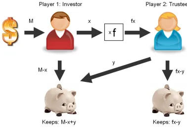
The trust game (Camerer and Weigelt 1988; Berg, Dickhaut et al. 1995) is a modified version of the dictator game (see Fig. 17): one player, the Investor, is endowed with M dollars and can invest any portion of it. The invested amount x is then multiplied by f, and the second player (the Trustee) decides how much of the resulting investment to keep and how much to pay back. The investor’s payoff is the amount originally held back, M-x, plus the returned money y. The Trustee’s payoff is fx-y. The collective gain is (M-x+y)+(fx-y)=M+(f-1)x which is maximized for x=M (when the Investor invests everything). Thus there is a significantly larger gain from cooperation.

Fig. 17: The trust game

According to game theory the best strategy in this game is for the Investor to invest nothing. Indeed, since the Trustee is trying to maximize his own earnings, he will not return any money, and thus there is no incentive for the Investor to invest.

interaction, where the multiplication of x represents productivity, the invested money amount x is a measure of trust, and the returned money amount y is a measure of trustworthiness. The repetitive nature of the trust game allows for multiple interactions between players, and thus more diverse and complex strategies. As players pass money between each other, they create (or break up) a mutual trust relationship based on reputation and previous history. The strength of that relationship can be measured in terms of reciprocity (this method will be explained in subsequent sections).

Although the repeated trust game is substantially more complex than its single-shot counterpart, the game-theoretic solution remains unchanged: the Investor should never invest money, and the Trustee should keep all the money that he receives. Indeed, the situation in the last round of the repeated trust game is exactly the same as it is in the single-round trust game, and neither player should invest/repay anything. Considering that nothing happens in the last round, the second-to-last round can now be considered to be the “last” round of the game, and the same reasoning applies. By reiterating this process backwards over all rounds, it follows that every round should be treated as a single-shot game, and that the Investor should never invest any money. For an initial endowment of

20

=

M , a multiplication factor f =3, and 10 rounds, the overall earnings will be

200 20

10x = (all earned by the Investor), which is considerably less than the maximum overall earnings from a cooperative strategy (10x20x3=600).

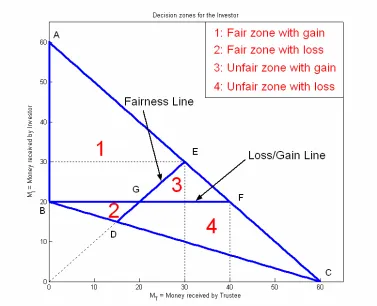
(for M =20, 3f = ): a round is defined to be fair if the Investor and the Trustee both earn the same amount of money.

Fig. 18: Fairness in the trust game

If the Investor invests at least 5, the Trustee can always return enough money to make the round fair. In some cases the Investor can end up with less money than his initial endowment, even though the Trustee divided the money in a fair way. In other cases he ends up with more than his initial endowment although the round was unfair. Figure 18 illustrates this from the point of view of the Investor. All possible money split-ups

) ,

(M_I M_T fall within the triangle ABC (where M_I is the money earned by the Investor and M_T is the money earned by the Trustee). Any money split-ups that fall on the segment

] ,

in Zone 2 (BDG), is also hyper-fair, but the Investor receives less than his initial endowment. Zones 3 (EFG) and 4 (CDGF) are both unfair, although in Zone 3 the Investor earns more money than his initial endowment (and thus still profits from the investment).

III.1.3. Previous Studies

All of the games mentioned in the previous sections have been studied extensively in behavioral economics (Camerer 2003), and with the recent availability of neuroscientific tools they become increasingly more popular in neuroeconomics.

McCabe et al. (McCabe, Houser et al. 2001) performed one of the earliest experiments in neuroeconomics by implementing a simplified version of the trust game. They found that subjects who played cooperative strategies have increased activity in the inferior frontal gyrus when playing against another person compared to when playing against a computer. In another implementation of the trust game, Delgado et al. (Delgado, Frank et al. 2005) modulated the investor’s a priori perception of the trustee’s moral character. They found that the caudate was differentially activated with respect to positive and negative feedback, but only when subjects were playing with the neutral partner. Kosfeld et al. (Kosfeld, Heinrichs et al. 2005) have also been able to artificially increase the level of trust in investors by intranasal administration of oxytocin, a neuropeptide that plays a key role in social attachment and affiliation.

their co-players, suggesting a first step towards understanding the mechanisms underlying social impairment. In another type of game Decety et al. (Decety, Jackson et al. 2004) studied the neural correlates of cooperation vs. competition, and found the orbitofrontal cortex to be more activated in the cooperation condition, and the inferior parietal and medial prefrontal cortices to be more activated in the competition condition. Sanfey et al. studied the neural correlates of unfairness in a ultimatum game (Sanfey, Rilling et al. 2003), and found that receiving unfair offers activated brain areas related to both emotion (anterior insula) and cognition (dorsolateral prefrontal cortex). Moreover, the activity in the insula was correlated with subject’s decision to reject the offer. In a more complicated design, subjects who received unfair offers were able to punish their partner by using some of their own money (de Quervain, Fischbacher et al. 2004). Punishments elicited activations in the dorsal striatum (a reward processing structure), and the level of activation was correlated with their willingness to incur greater loss in order to punish. Although a couple of neuroimaging studies have investigated a simplified version of the trust game, the work presented in this thesis is the first to analyze the neural correlates of the repeated trust game in interacting subjects.

III.2. Experimental Design and Methods

III.2.1. Task

had no knowledge of the actual pay scale, but were informed that they could earn $20–40 based on their performance.

III.2.2. Subjects

To assure anonymity, subjects were recruited from separate subject pools at the California Institute of Technology (CIT), Pasadena, CA and Baylor College of Medicine (BCM), Houston, TX. Informed consent was obtained by using a consent form approved by the Internal Review Boards of both CIT and BCM. Investor/Trustee roles were assigned pseudo-randomly, and subjects were matched for gender, location and player role to control for confounding effects. Specifically, there were 12 subject pairs of each combination MM, MF, FM, FF where M=Male player and F=Female player, the first subject listed denoting the Investor and the second one the Trustee. There were a total of 48 subject pairs.

III.2.3. Experimental Setup

The behavioral and functional data in the trust game was acquired using the NEMO hyperscanning software (Montague, Berns et al. 2002), which simultaneously recorded BOLD responses in interacting subjects (Fig. 19). Subjects were instructed identically, but separately at each location (instructors read a script describing the task while showing screenshots of the game).

Fig. 19: Hardware setup of the trust game

The timeline of a single round of the trust game is depicted in Fig. 20. Each round starts with a blank screen that lasts 4 seconds, followed by a free response period where the Investor decides how much money to invest. During that period the Trustee sees a blank screen. 8 seconds after the Investor submits his decision, the results of the investment phase are revealed to both subjects simultaneously. Then the repayment phase starts where the Trustee decides how much to send back to the Investor and how much to keep. During that time the Investor sees a blank screen. 8 seconds after the Trustee’s decision the results of the repayment phase are revealed simultaneously to both players. After another 8 second blank screen a summary with the overall totals for the round is revealed to both subjects. Each round is separated from the next one by a blank screen of random duration (12–42 seconds). Note that except for the periods of free response both players view the same visual stimulus.

III.2.4. fMRI Data Acquisition and Preprocessing

Brain image acquisition was done on a Siemens Trio (CIT) and a Siemens 3T Allegra (BCM). High resolution T1-weighted scans (0.48 mm x 0.48 mm x 1 mm) were acquired using a MPRage sequence. Functional images were acquired using echo-planar T2* images with BOLD contrast. Parameters were as follows: repetition time (TR) = 2000 ms; echo time (TE) = 40 ms; slice thickness = 4 mm yielding in a 64x64x26 matrix (3.4 mm x 3.4 mm x 4 mm); flip angle = 90 degrees; FOV read = 220 mm; FOV phase = 100 mm, series order: interleaved.

III.3. Behavioral Results

Since subjects were free to invest/return as much money as they wanted in each round, there was a lot of inter-pair variability, resulting in a rich behavioral space. A few examples of typical money exchanges are presented below.

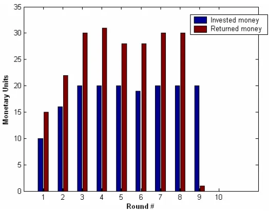
Fig. 21: Example #1 of monetary exchange

Figure 21 shows the interaction between two cooperating subjects. The Investor invests his whole endowment in every round, and the Trustee repays his trust by splitting the money equally between the two. In round 9 however the Investor invests nothing, as he is probably worried that the Trustee might not pay anything back this close to the end of the game. The Investor seems to have done two steps of iterated reasoning with respect to the game-theoretic solution.

time it was the Trustee who did the 2 steps of iterated game-theoretic reasoning. In response to the betrayal the Investor invests nothing in Round 10.

Fig. 22: Example #2 of monetary exchange

Fig. 23: Example #3 of monetary exchange

Investor invests nothing in Round 7. The Investor seems to be forgiving as he starts investing again in round. Typically players give their opponent a second chance if they split the money in an unfair way. Also note that in this example neither player takes all the money in the last round(s) unlike in the two previous examples.

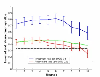
The average behavior of all 48 subject pairs is shown in Figure 24. Cooperation between players was the strongest during middle rounds: trusting behavior (identified by large investment ratios), peaked during round 6 when Investors invested an average of 81% of the available money, and trustworthiness (identified by large repayment ratios) peaked in round 4 when Trustees returned an average of 47% of the invested money.

After these peaks, both investment and repayment ratios declined over rounds, reflecting a decrease in cooperation. They reached their lowest value in the last round, which was also the only round where investments did not earn a profit on average (the repayment ratio is lower than 1/3). No Investor played the perfectly selfish Nash equilibrium in which the Investor invests nothing in each round. On average Investors earned $256.54 +/- 56.08 and Trustees earned $237.58 +/- 63.42, both resulting in an actual payoff of $35.

III.4. Strategic Uncertainty and Prediction Analysis

III.4.1. Background

Human social life depends on the ability to predict the likely behavior of others, a capacity that underlies cooperation and social institutions (Henrich, Boyd et al. 2005). Unlike individual decision-making under uncertainty, the hallmark of decision-making in social interactions is strategic interdependence. That is, one’s best strategy depends on the strategy others adopt, often in response to one’s own behavior. This strategic interdependence introduces a novel form of uncertainty, referred to as strategic uncertainty, which is the uncertainty associated with inferring the beliefs and possible actions of others. In most social interactions, we lack perfect information about what others believe, and so lack perfect foresight about how others will respond to our own behavior, creating uncertainty about our predictions. Because of this, strategic uncertainty is a pervasive feature of human strategic interaction—including negotiation, international relations, and trading in such institutions as asset markets—and remains even when all other sources of uncertainty (structural uncertainty) surrounding a decision context are removed (Brandenburger 1996).

others. Such work has identified the anterior paracingulate, superior temporal sulci, and temporal poles as regions implicated in ToM (Fletcher, Happe et al. 1995; Goel, Grafman et al. 1995; Baron-Cohen, Ring et al. 1999; Gallagher, Happe et al. 2000). While ToM is thought to have evolved as a capacity to predict the behavior of others through the attribution of mental states that play a role in generating behavior (Premack and Woodruff 1978), ToM can be invoked in situations that do not involve strategic interaction and predictions of future behavior. For example, understanding some forms of humor and retrospectively explaining behavior may require mentalizing abilities but does not involve strategic interaction in the sense that the required mentalizing does not involve predicting a future response to one’s own behavior (Gallagher, Happe et al. 2000). For this reason, many ToM studies utilize tasks that require subjects to retrospectively judge a social scenario in which they are not directly involved, thus evoking social, but not strategic, interaction. Thus, while ToM is the capacity to attribute mental states generally, strategic uncertainty is more specifically a form of prediction risk, namely the uncertainty associated with the future response to one’s own behavior. Investigation of strategic uncertainty thus requires tasks in which subjects strategically interact with one another, rather than make social judgments retrospectively.

whereas reported activations related to ToM have been cortical, this thesis examines whether strategic uncertainty in a high-level social exchange may evoke similar subcortical structures.

A further salient difference between ToM and strategic uncertainty is that strategic uncertainty is quantifiable, whereas ToM typically is not. Since strategic uncertainty is the predictability of a decision-maker’s response to one’s decision, this predictability can be quantified by the entropy of one’s strategic choice, as different strategies often differ in the predictability of the response they will evoke. For example, when a car dealership advertises the purchase price of a car, both very high and very low prices involve relatively little strategic uncertainty, since very high prices have a low probability of acceptance and very low prices have a very high probability of acceptance. If the car dealership is motivated to sell the car for the highest possible price, the task becomes that of predicting the highest price that will be accepted, which will involve relatively high levels of strategic uncertainty. Thus, a goal of this study was to examine whether the entropy of different strategies related in a parametric manner to the magnitude of neural activations, which would provide strong evidence that such activations encoded strategic uncertainty.

players modify their strategic behavior by calibrating strategic uncertainty as they learn from responses of others across repeated plays.

Based on the above considerations, we investigated strategic uncertainty in the trust game. Specifically, we examined whether there are brain signals that both reflect strategic uncertainty as a function of strategic learning in previous rounds and predict future strategic choice.

III.4.2. GLM Analysis: New vs. Known Information

The structure of the finitely repeated trust game requires subjects to modify their strategic behavior as the game evolves and information in the form of opponent responses becomes available. In particular, two critical moments of a round influence strategic choice: the revelation of the results from the investment and repayment phases.

Cluster Voxel Area

pcor kE punc pFWE pFDR T (Z) X Y Z L/R Area

0.042 163 0.023 0.001 0.003 5.99 5.14 3 9 48 R Sup. Fr. Gyrus, BA6/8 0.099 109 0.057 0.004 0.003 5.63 4.90 9 3 0 Caudate

0.026 0.004 4.97 4.43 21 9 -6

0.288 49 0.186 0.004 0.003 5.60 4.87 -42 21 -15 L Orbitofr. Cortex, BA47 0.012 0.003 5.26 4.64 -33 18 -15

0.238 59 0.149 0.008 0.003 5.39 4.73 -9 6 0 L Caudate

0.387 34 0.267 0.024 0.004 5.00 4.46 -27 -99 0 L Visual Cortex 0.189 0.012 4.21 3.85 -33 -93 -6

0.687 0.045 3.49 3.27 -15 -99 0

0.149 85 0.088 0.027 0.004 4.96 4.42 0 36 -12 Med. Fr. Gyrus, BA11/32 0.517 0.030 3.69 3.44 12 30 -12 R

0.676 0.044 3.50 3.28 0 54 -6

0.494 22 0.373 0.091 0.008 4.50 4.09 36 15 -15 R Orbitofr. Cortex, BA47

0.599 13 0.499 0.117 0.009 4.40 4.01 45 -84 -3 R Visual Cortex

0.317 44 0.209 0.194 0.013 4.19 3.85 6 -93 -6 R Visual cortex 0.362 0.020 3.90 3.61 24 -99 -6

0.464 25 0.341 0.203 0.013 4.17 3.83 -3 -27 -3 L Midbrain

Although the revelation screens are visually identical, the displayed information is asymmetric in that for the Trustee the investment screens contains new information (the amount invested by the Investor) whereas the repayment screen displays known information (note that this is exactly the opposite for the Investor). As this new information is the basis for subsequent strategic behavior, we defined two regressors of interest, βinv and

βrep, corresponding to the revelation of the investment and repayment screens respectively. A general linear model (GLM) analysis was used to identify brain areas in the Trustee brain whose blood oxygenation level-dependent (BOLD) response was greater for the information bearing screen than for the known screen (see Section III.4.8 for methods).

Fig. 25: Activations in the Trustee Brain. (A) Left panel: coronal view (y=0) of the Trustee brain showing significant differential activation in the bilateral caudate for the contrast βinv - βrep. A

Five regions, all previously implicated in reward-processing and decision-making (Schultz, Dayan et al. 1997; Cohen, Botvinick et al. 2000; Elliott, Friston et al. 2000; Paulus, Hozack et al. 2002; Delgado, Miller et al. 2005), showed significant activation and were used as regions of interest (ROI) for subsequent analysis: bilateral caudate; medial midbrain; superior frontal gyrus (BA6/8), bilateral orbitofrontal cortex (BA47) and medial frontal gyrus (BA11/32) (Table 1 and Figure 25).

III.4.3. ROI Analysis: Correlation between Later Decisions and Hrf

We next investigated whether activation in these ROIs was correlated with subsequent Trustee responses to Investor behavior (see Section III.4.8. for methods on ROI analysis). Consequently, we examined future changes in repayment ratio ΔR_ias a function of current changes in investment ratio ΔI_i (Fig. 26).

Fig. 26: Split-up of the behavioral space. Green quadrants contain reciprocal events and red quadrants contain anti-reciprocal events. Neutral events are located at (0,0) in the blue disk. Subpanels show the average Investment (blue) and Repayment (red) ratios in each quadrant for rounds i-1 and i. The blue and red arrows show the direction of the corresponding changes in Investment and Repayment ratios respectively (e.g., in the top-left quadrant the Investor increases his investment ratio, and the Trustee subsequently decreases his repayment ratio).

similarity between caudate and midbrain time-courses led me to conclude that the midbrain activation was reliable.

in bilateral caudate and midbrain during middle (3–6) rounds. We segregated signals in response to the revelation of the investment screen (t=0) with respect to reciprocal (green), non-reciprocal (red), and neutral (blue) strategies (significance levels: p<0.05: *, p<0.005: **, R vs. N: green stars, N-R vs. N: red stars, N-R vs. R: black stars). Since the actual repayment phase only starts 22 seconds later, the time-courses are predictive of the trustee’s strategy. Right panel: entropy of the Investor’s next move as a function of strategy (Hreciprocal, Hnon-reciprocal, Hneutral). High entropy values denote high uncertainty levels. These data show that during middle rounds Hreciprocal > Hnon-reciprocal > Hneutral, which is exactly the same order as signal magnitudes in the left and middle panels. (B) Similar as in (A), we segregated signals in the caudate (left panel) and midbrain (middle panel) according to strategy in late (7–10) rounds. During late rounds it is no longer possible to distinguish between reciprocal and non-reciprocal strategies. This trend is also repeated in the uncertainty of the Investor’s next move, where Hnon-reciprocal has increased to the level of Hreciprocal. This change in both signal magnitude and entropy from middle to late rounds suggests that signal magnitude in the caudate and midbrain encodes for uncertainty about the Investor’s future moves.

During middle rounds time-courses for all three strategies had different peaks: reciprocal events had the largest magnitudes and neutral events had the lowest. By late rounds the amplitude of non-reciprocal events had risen to the level of reciprocal events. This difference between signals across late and middle rounds confirmed the hypothesis regarding strategic learning and the opportunity for players to learn about their opponents in contexts that encouraged reciprocity (Fehr and Gachter 1998) (repeated play of the middle rounds), or discouraged reciprocity (the shadow of the game’s end, a phenomenon known as endgame effects, which are well-established empirically in behavioral game theory (Camerer and Weigelt 1988; Dal Bo 2005).

III.4.4. Signal Magnitude Encodes Strategic Uncertainty

tested the alternative hypothesis that signal magnitude encodes the uncertainty of future reward, or strategic uncertainty, i.e., the predictability of the next investment after the Trustee’s repayment decision, which can be measured by entropy (Shannon 1948) (see Section III.4.8. for methods). We found a correspondence between the relative magnitudes of brain signals in midbrain and caudate and the entropy of different strategies in middle rounds (rightmost panels in Fig. 27). Both signal magnitude and entropy are the highest for reciprocal events, and the lowest for neutral events. During late rounds the entropy of non-reciprocal events increased to the level of non-reciprocal events, as did the signal magnitude in midbrain and bilateral caudate (left and middle panels in Fig. 27). This relationship provided further support that the late rounds induce different strategic interactions due to increasing strategic uncertainty as the end of the game draws near. Although players did not fully follow backward induction as predicted by analytical game theory (Camerer 2003), by late rounds they anticipated the final round, reducing the incentive for reciprocity. The correspondence between entropy and signal magnitudes across events in the middle periods, and the increase in both entropy and signal for non-reciprocal events from middle to late periods, strongly suggest that these brain areas encode Trustee strategic uncertainty as measured by entropy.

III.4.5. Signal Magnitude Predicts Future Strategic Choice