Article
Managing Real Power Loss of Distribution System
Connected with Distributed Generator Using Least
Square Quadratic Approximation
Komson Daroj
Department of Electrical and Electronics Engineering, Faculty of Engineering, Ubon Ratchathani University, 85 Satholmark Rd., Warinchamrap District, Ubonratchathani 34190, Thailand
E-mail: [email protected]
Abstract. This paper compared two scenarios for managing real power loss of a distribution feeder connected with a Distributed Generator (DG). Under planning scenario, the objective is to obtain the optimal purchasing contract, which is a constant power injected from DG to minimize loss of a feeder. In real time operating scenario, the optimal scheduled power of DG to minimize loss for each hour is calculated. These two scenarios are formulated as optimization problems and solved with the proposed Least Square Quadratic Approximation (LSQA) technique. This technique is formulated based on a quadratic nature of a real power loss versus its real power output injected from DG. In term of the obtained results, it is reliable and has high accuracy. A 93-bus radial distribution system connected with a synchronous based DG sizes 7.5 MW under North-Eastern region 2 of Provincial Electricity of Thailand (PEA) is adopted as a tested system. The obtained results shown that managing loss under both scenarios bring benefits to a tested feeder. Moreover, the proposed LSQA technique is easy to understand, thereby can be used alternatively with others present optimization techniques.
Keywords: Distributed generator, least square approximation, real power loss, distribution system, optimal capacity.
ENGINEERING JOURNAL Volume 21 Issue 6 Received 28 August 2017
1.
Introduction
High penetration of DG connected in a distribution system has significance impacts to the end customers in term of reliability and quality of supply [1], [2]. To compatible with the unpleasant impacts from DG, this circumstance required for administered strategies and technologies. For example, the used of advanced inverter technologies, Static Var Compensator (SVC), and Energy Storage (ES) system can solve the problem of voltage fluctuations occurred from an intermittent resource nature of Photovoltaic (PV) and Wind Turbine (WT) plants. However, these technologies are not mature and rely on them has an expensive cost [3]. In contrast with mitigating some disadvantages from a feeder connected with high penetration of DG, gaining the benefits use from DG to reduce real power loss of a system is of interested [4]. Consequently, launching the appropriate policies and regulations for mitigating unsuitable impacts, meanwhile accommodating several benefits use of DG are respectable strategies. This can be done through both the planning and real time operating stages. The achievement depends on several factors e.g., the government policies, proper utility’s regulations, and the structure of electric supply industry.
The real power loss and voltage profile of a distribution feeder connected with DG depend on various factors e.g., type, size, and location of DG and also the profile of loads distributed along a feeder [5], [6]. The size of DG has limit by technical factors e.g., capacity of a primary distribution line, short circuit level, and reliability and quality impacts. The intervened policy by rewarding or penalizing DG’s owner due to the proper size and location of DG in planning stage can be found in literature [7] however it still not be implemented in any utility. For some countries like Thailand, almost of DGs under VSPP (Very Small Power Producer) program is normally invested by private sectors without intervention from the government agencies [8]. Therefore, gaining benefits of DG by governing its size and location as proposed in [7] cannot be implemented at present stage. In the future, this situation may be changed due to drastically increasing penetration level of DG and their impacts to the end customers in a system.
The methodologies for reducing distribution real power loss of a system connected with DG under operating stage attracted much attention. This can be implemented under several programs e.g.: demand side management, demand response, and peak demand shaving programs [9]. In UK, the Distribution Network Operator (DNO) is reward or penalized for the loss lower or higher than the target. This regulation support DNO to perform mechanism to manage loss by using; i) call on customers who have backup generators during peak periods, and ii) perform DG dispatch programs to supply peaking, reserve or load management capability [10].
In this paper, the LSQA algorithm is proposed to solve an optimization problem of managing real power loss. The methodology of LSQA relies on a quadratic nature between the real power injected from DG and its associated real power loss in a distribution feeder. The frameworks of managing loss are formulated as an optimization problem, which can be classified into two sub-problems i.e., planning with the optimal capacity contract and the optimal dispatching real power of DG under real time operating stage problems. The advantage of the proposed LSQA is easy for understanding when compare with others optimization techniques. The proposed methodology is tested with a 93-bus radial feeder connected with a DG sized 7.5 MW. The obtained results provide the satisfactory of reducing real power loss both under planning and real time operating stages
2.
Impact of DG Power to Real Power Loss
In a transmission system, at a specified time, real power loss can be simplified into a quadratic equation of the generated power. This relationship can be represented as a matrix called B coefficient matrix, which is classically use for Economic Dispatch (ED) and Optimal Power Flow (OPF) problems [11]. This relationship has more strong in a primary distribution than a transmission systems due to limitation of control variables and the absent of parallel flow path. For any voltage control mode of DG i.e.: constant power factor, constant voltage, and constant reactive power, real power loss can be approximated from (1).
2Loss G G
P a P bP c (1)
3.
The LSQA [12]
Given the scripts G, P, Loss and n are denoted for DG bus, real power, real power loss and a number of snap shot data between PG and its associated real power loss respectively. The LSQA is proposed to represent the quadratic nature relationship between generated power from DG and the real power loss of a distribution feeder, which can be formulated as follow:
(i) Generate n series of points between the generated power from DG and its associated distribution loss;
i i
Loss G
P ,P , using a power flow equation,
(ii) From (i), the function of the sum square of the loss deviation for n number of coordination pairs can be illustrated as (2)
21 , , , , Loss n i i
F a b c P a b c
, (2)where
Loss i
P
a,b,c
is a loss deviation function obtained from the predicted loss formula and the loss obtained from a power flow equation, which can be stated in (3)
2
, ,
Loss
i i i i
G G Loss
P a b c P a P b c P
, (3)
(iii) To obtain the coefficients a, b, and c from (2) satisfied the minimal condition, the gradient of (2) respect to these coefficient must be zero as below
2 1 1 12 , , 0
2 , , 0
2 , , 0
Loss Loss Loss n i i G i n i i G i n i i
P P a b c
P P a b c
P a b c
, (4)
(iv) Rearranged Eq. (4) and represented in a matrix form as (5)
4 3 2 2
1 1 1 1
3 2
1 1 1 1
2
1 1 1
n n n n
i i i i i
G G G Loss G
i i i i
n n n n
i i i i i
G G G Loss G
i i i i
n n n
i i i
G G Loss
i i i
P P P P P
a
P P P b P P
c
P P n P
, and (5)
(v) Equation (5) can be solved easily to obtained the coefficients a, b, and c, and
(vi) Eventually the generated power from DG; PG, that resulted in the minimal loss is –b/2a.
4.
Calculation Algorithm
(i) Generate three pairs of data between the generated power from DG and its associated distribution loss,
1 1
2 2
Loss Loss
G G
P ,P , P ,P , and
3 3
Loss G
P ,P using a power flow calculation.
(ii) Calculate the approximated optimal PG as described in section 3 and its associated real power loss. (iii) Replace the optimal PG and its associated real power loss to the most deviated previous data. (iv) Repeat until the convergence criterion is satisfied.
The formulation of LSQA in (3) is not limit to a real power loss function. It can be applied further to an energy loss function of summing the product between real power loss and time step of all specified periods.
5.
Optimization Framework
5.1. Objective Function
The objective function of the both scenarios of managing loss under planning and operating stages is the same as shown in (6).
1
T t Loss Loss
t
Minimize E P T
, (6)The variables t is denoted for a specified period of time.
5.2. Common Constraints
The common constrains of the both scenarios are
1
, i, j N, t T
i schi
N
t t t t
sch ij ij
j
P jQ P jQ
, (7)min max
, t T
t
G G G
Q Q Q , and (8)
min max
, k N, t T
t
k k k
V V V ,. (9)
Scripts N and T are denoted for a number of buses in a system and a number of time periods respectively. The equality constraint as stated in (7) is a power flow equation. The inequality constraints as stated in (8) and (9) are to ensure that reactive power of DG and system voltage profiles are regulated within an acceptable range.
5.3. Characteristic Constraints
The control variables of the two scenarios for managing real power loss are difference. Accordingly, their associated constraints satisfying the objective function of (6) have their own character, which can be described below.
Under planning stage, assumed that DG supplied power at an optimal purchasing contract, Opt G
P ,
which is a constant power injected from DG at all specified period as shown in (10).
, t T
t Opt G G
P P , (10)
Under operating stage, the scheduled power from DG is assumed to be controlled optimally within an acceptable range as shown in (11) to minimize the real power loss for each period.
min t max, t T
G G G
6.
Test System
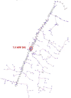
Topology of the 93-bus radial distribution system connected with a synchronous DG capacity of 7.5 MW at bus No. 42 as shown in Fig. 1 is used as a tested system. A daily load profile of this system with peak demand of 6.42 MW is shown in Fig. 2.
Fig. 1. Network topology of a 93-bus radial distribution system.
Fig. 2. Daily load profile of a tested system. 0
5 10
15
20 24
0 10 20 30 40 50 60 70 80 90 0 50 100 150 200 250 300 350 400 450 500
Hour Bus No.
[image:5.595.150.449.141.555.2] [image:5.595.175.421.588.749.2]7.
Numerical Results
7.1. Base-case Characteristics
Two based-cases i.e., cases with and without a 7.5 MW DG are simulated in this section. The voltage magnitude of a substation and a DG buses are set as 1.02 and 1.05 p.u. respectively. The obtained result of voltage profiles can be shown in Fig. 3 and Fig. 4.
Fig. 3. System voltages in case of without DG.
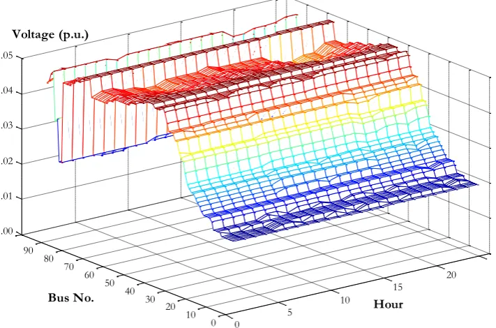
From Fig. 3, magnitude of the voltage in the system is slightly decreased from the substation bus to the remote end buses. For groups of bus located at the remote end side, they have voltage magnitude less than a lower bound of an unacceptable range. This profile is changed due to the presence of DG at bus No. 42. At this bus, the voltage is pulled up to its set point. Consequently, the voltage magnitude of the overall system is improved as shown in Fig. 4.
Fig. 4. System voltages in case of connecting with a DG capacity of 7.5 MW.
0 5
10
15 20
24
0 10 20 30 40 50 60 70 80 90 0.90 0.91 0.92 0.93 0.94 0.95 0.96 0.97 0.98 0.99 1.00 1.01 1.02
Bus No. Hour
Voltage (p.u.)
0 5
10
15 20
0 10 20 30 40 50 60 70 80 90 1.00 1.01 1.02 1.03 1.04 1.05
Voltage (p.u.)
[image:6.595.123.474.171.410.2] [image:6.595.123.479.511.746.2]Hourly real power loss of these two cases, without DG and with DG, can be shown in Fig. 5
0 0.1 0.2 0.3 0.4 0.5 0.6
1 2 3 4 5 6 7 8 9 10 11 12 13 14 15 16 17 18 19 20 21 22 23 24 No. DG
7.5 MW DG
Fig. 5. Hourly power loss of a system.
From Fig. 5, due to the presence of DG, the real power losses are increased during the low load hours from 23:00 – 05:00 and 08:00 – 17:00 and the losses are decreased during the intermediate load and the high load hours from 06:00 – 07:00 and 18:00 – 22:00 respectively. In term of daily energy loss, it is increased from 4.764 to 5.841 MWh.
7.2. The Optimal Purchasing Contract
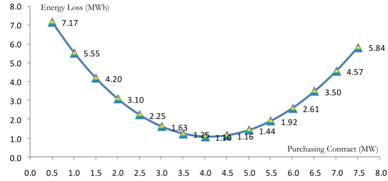
To mitigate disadvantage of DG to energy loss of the system, the optimal purchasing contract has to be evaluated. For the location of DG at bus No. 42, the relationship of the quantity of real power signed in the purchasing contracts versus its associated daily energy loss can be shown in Fig. 6.
5.84
4.57
3.50
2.61 1.92
1.44
1.16 1.10 1.25 1.63 2.25 3.10 4.20 5.55 7.17
0.0 1.0 2.0 3.0
4.0 5.0
6.0 7.0 8.0
0.0 0.5 1.0 1.5 2.0 2.5 3.0 3.5 4.0 4.5 5.0 5.5 6.0 6.5 7.0 7.5 8.0
Fig. 6. Quantity of the purchasing contract to the energy loss.
From the quadratic relationship illustrated in Fig. 6, the optimal power of the purchasing contract is between 4.00 -5.00 MW. To clarify, the LSQA technique described in section 3, a numerical example by using three points of purchasing contract 3.5, 4, and 4.5 MW as shown in Fig. 6 is presented as follow;
(i) Generate three points of the data between generated power from DG (MW) and its associated energy loss (MWh) i.e.,
3.5,1.254195 , 4.0,1.098839
, and
4.5,1.162539
,(ii) The function of the sum square of the energy loss deviation can be shown in (12) Energy Loss (MWh)
Purchasing Contract (MW) Power Loss (MW)
[image:7.595.137.467.119.298.2] [image:7.595.94.494.467.654.2]
2 2 2 2 2 23.5 3.5 1.254195 4 4 1.098839
, ,
4.5 4.5 1.162539
a b c a b c
F a b c
a b c
(12)
(iii) The partial derivative of F a,b,c
respect to a, b and c can be shown in (13) – (15) respectively,
2 2 2 2 2 2 2 2 22 3.5 3.5 3.5 1.254195
, ,
2 4 4 4 1.098839
2 4.5 4.5 4.5 1.162539
a b c
F a b c
a b c
a
a b c
(13)
2 2 2 2 2 22 3.5 3.5 3.5 1.254195
, ,
2 4 4 4 1.098839
2 4.5 4.5 4.5 1.162539
a b c
F a b c
a b c
b
a b c
(14)
2 2 2 2 2 22 3.5 3.5 1.254195
, ,
2 4 4 1.098839
2 4.5 4.5 1.162539
a b c
F a b c
a b c
b
a b c
(15)
Terms from Eq. (13) – (15) must be zero to satisfy the minimal condition, thus
2 22 2 2 2
2 2 2 2 2 2 2 2 2 2 2 2
3.5 3.5 3.5 1.254195 4 4 4 1.098839
0
4.5 4.5 4.5 1.162539
3.5 3.5 3.5 1.254195 4 4 4 1.098839
0
4.5 4.5 4.5 1.162539
3.5 3.5 1.254195 4
a b c a b c
a b c
a b c a b c
a b c
a b c a
2 2 2 4 1.098839 04.5 4.5 1.162539
b c
a b c
, (16)
(iv) Rearrange Eq. (16), it can be represented in a matrix form as (17)
816.1250 198.000 48.500 56.486727
198.000 48.500 12.000 14.016464
48.500 48.500 3 3.515573
a b c
, (17)
(v) Solve Eq. (17), the coefficients a, b, and c, are 0.438112, -3.596551 and 8.475252 respectively, (vi) PG that resulted in the minimal loss can be calculated from –b/2a, which is 4.104603 MW.
Table 1. Energy loss equation fit with different a number of points.
Number of
Points Energy Loss Equation
Opt G
P
(MW)
Energy Loss (MWh)
3 0.43811P2 - 3.59655P + 8.47525 4.104603 1.09424554
5 0.43833P2 - 3.60314P + 8.49805 4.110077 1.09426805
7 0.43867P2 - 3.61305P + 8.53225 4.118187 1.09434938
9 0.43911P2 - 3.62631P + 8.57782 4.129159 1.09455057
11 0.43967P2 - 3.64295P + 8.63475 4.142823 1.09494755
13 0.44035P2 - 3.66302P + 8.70302 4.159214 1.09563781
15 0.44114P2 - 3.68656P + 8.78258 4.178447 1.09674528
From Table 1, the accuracy of the solution is not depends on the number of points but depends on proximity of points used in the prediction. By applying a three-point set cutting algorithm as presented in section 3, the accurate energy loss equation can be shown in (18).
2
0.43367 3.55833 8.39347
Loss G G
E P P , (18)
From Eq. (18), the optimal purchasing contract is 4.10258 MW with its associated energy loss of 1.09424 MWh.
7.3. The Optimal Real Time Scheduling
The optimal real power scheduling from DG is conducted in real time separately for each hour as stated in section 5.3. After apply a three-point set cutting algorithm described in section 3, the optimal PG at each hour can be shown in Fig. 7. As a result, the associated energy loss under this scenario is 0.83502 MWh. It obviously found that this value is lower than the case of using the optimal purchasing contract, which is 1.09424 MWh.
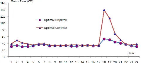
The comparison of the hourly real power losses between these two scenarios is shown in Fig. 8. In conclusion, during the low and high load periods from18:00 – 05:00, the real energy losses obtained from the optimal scheduling power method are significant lower than the value obtained from the optimal purchasing contract method. Meanwhile, the real energy losses from 05:00 – 18:00 obtained from both scenarios are quite similar.
8. Conclusions
Fig. 7. Optimal real power of DG scheduling at each hour.
Fig. 8. Comparison of the real power loss for each hour.
References
[1] R. C. Dugan, T. E. McDermott, and G. J. Ball, “Planning for distributed generation,” IEEE Industry Application Magazine, vol. 7, no. 2, pp. 80–88, Mar./Apr. 2001.
[2] J. A. Greatbanks, D. H. Popovic, M. Begovic, A. Pregelj, and T. C. Green, “On optimization for security and reliability of power systems with distributed generation,” presented at IEEE Bologna Power Tech Conference, Bologna, Italy, Jun. 23–26, 2003.
[3] J. A. Pec, A. Lopes, N. Hatziargyriou, J. Mutale, P. Djapic, and N. Jenkins, “Integrating distributed generation into electric power systems: A review of drivers, challenges and opportunities,” Electric Power System Research, vol. 77, no. 9, pp. 1189–1203, Jul. 2007.
[4] H. A. Gil and G. Joos, “Models for quantifying the economics benefits of distributed generation,” IEEE Transactions on Power Systems, vol. 23, no. 2, pp. 327-335, May 2008.
[5] W. El-khattam, Y. G. Hegazy, and M. M. a Salama, “An integrated distributed generation optimization model for distribution system planning,” IEEE Transaction on Power System, vol. 20, no. 2, pp. 1158– 1165, 2005.
[6] V. H. M. Mandez, J. R. Abbad, and T. G. S. Roman, “Assessment of energy distribution losses for increasing penetration of distributed generation,” IEEE Transactions on Power Systems, vol. 21, no. 2, pp. 533-539, May 2006.
[7] S. N. G. Naik, D. K. Khatod, and M. P. Sharma, “Analytical approach for optimal siting and sizing of distributed generation in radial distribution networks,” IET Generation, Transmission & Distribution, vol. 9, no. 3, pp. 209–220, 2015.
[8] Ministry of Energy. (2016). Energy Policy and Planning Office (EPPO). [Online]. Available: http://www.eppo.go.th/index.php/en/
[9] U.S. Department of Energy, Federal Energy Management Program. (2002, May). Using Distributed Energy Resources. [Online]. Available: http://www.eren.doe.gov/femp/
[10] P. Siano, L. F. Ochoa, G. P. Harrison, and A. Piccolo, “Assessing the strategic benefits of distributed generation ownership for DNOs,” IET Generation Transmission and Distribution, vol. 3, pp. 225-236, Mar. 2009.
[11] A. J. Wood and B. F. Wollenberg, Power Generation Operation and Control, 2nd. ed. John Wiley & Sons,
1996.
[image:10.595.179.416.86.196.2] [image:10.595.176.417.231.340.2]