This is a repository copy of
Coordinate descent iterations in fast affine projection algorithm
.
White Rose Research Online URL for this paper:
http://eprints.whiterose.ac.uk/695/
Article:
Zakharov, Y orcid.org/0000-0002-2193-4334 and Albu, F (2005) Coordinate descent
iterations in fast affine projection algorithm. IEEE Signal Processing Letters. pp. 353-356.
ISSN 1070-9908
https://doi.org/10.1109/LSP.2005.843765
[email protected] https://eprints.whiterose.ac.uk/
Reuse
Items deposited in White Rose Research Online are protected by copyright, with all rights reserved unless indicated otherwise. They may be downloaded and/or printed for private study, or other acts as permitted by national copyright laws. The publisher or other rights holders may allow further reproduction and re-use of the full text version. This is indicated by the licence information on the White Rose Research Online record for the item.
Takedown
If you consider content in White Rose Research Online to be in breach of UK law, please notify us by
Coordinate Descent Iterations in Fast Affine
Projection Algorithm
Yuriy Zakharov
, Member, IEEE,
and Felix Albu
, Member, IEEE
Abstract—We propose a new approach for real-time imple-mentation of the fast affine projection (FAP) algorithm. This is based on exploiting the recently introduced dichotomous coor-dinate descent (DCD) algorithm, which is especially efficient for solving systems of linear equations on real-time hardware and software platforms since it is free of multiplication and division. The numerical stability of the DCD algorithm allows the new combined DCD-FAP algorithm also to be stable. The convergence and complexity of the DCD-FAP algorithm is compared with that of the FAP, Gauss–Seidel FAP (GS-FAP), and modified GS-FAP algorithms in the application to acoustic echo cancellation. The DCD-FAP algorithm demonstrates a performance close to that of the FAP algorithm with ideal matrix inversion and the complexity smaller than that of the Gauss–Seidel FAP algorithms.
Index Terms—Coordinate descent, echo cancellation, fast affine projection, Gauss–Seidel algorithm.
I. INTRODUCTION
T
HE affine projection (AP) algorithm is an efficient adap-tive filtering technique [1]. It allows a higher convergence speed than the normalized least-mean squares (NLMS) algo-rithm, especially when the excitation signal is colored, as is the case with speech. However, it is complicated for implementa-tion. The fast AP (FAP) algorithm allows a significant simpli-fication [2], but it requires matrix inversion, which is a source of numerical instability, especially when implementing on real-time hardware [e.g., field-programmable gate array (FPGA)] and fixed-point software [e.g., digital signal processor (DSP)] platforms. In the original FAP algorithm, this is due to the fast recursive least-squares (RLS) algorithm. Other iterative tech-niques were proposed for matrix inversion in the FAP algorithm, in particular, the steepest descent and conjugate gradient tech-niques [3]. Gauss–Seidel (GS) iterations provide a good solu-tion to the problem; one GS iterasolu-tion per sample is enough in order to achieve nearly optimal performance [4], [5]. The FAP algorithm based on matrix inversion is computationally efficient only if the step size, which controls the convergence speed and the steady-state output (residual) error, is close to one. To re-duce the residual error after the algorithm has converged, the step size should be reduced. Moreover, when the step size is close to one, the FAP algorithm is sensitive to the input noise.Manuscript received June 29, 2004; revised November 11, 2004. This work was supported in part by the European Commission under CAPANINA Project FP6-IST-2003-506745. The associate editor coordinating the review of this manuscript and approving it for publication was Prof. Zhi Ding.
Y. Zakharov is with the University of York, York, YO10 5DD U.K. F. Albu is with the Politehnica University of Bucharest, Bucharest, 060032 Romania.
Digital Object Identifier 10.1109/LSP.2005.843765
As a result, there is still a necessity to find an efficient numer-ical implementation of the FAP algorithm with an arbitrary step size.
We propose a new approach for real-time implementation of the FAP algorithm. This is based on exploiting the recently in-troduced dichotomous coordinate descent (DCD) algorithm [6] for solving systems of linear equations. The numerical stability of the DCD algorithm allows the new combined DCD-FAP al-gorithm also to be stable. The DCD alal-gorithm is free of multi-plication and division. Its complexity is low compared with the whole complexity of adaptive filtering. We compare the perfor-mance of the new algorithm with the NLMS algorithm, the FAP algorithm based on an ideal matrix inversion (ideal FAP) or GS iterations (GS-FAP), and a modified GS-FAP algorithm based on the solution of a linear system in application to acoustic echo cancellation.
II. FAP ALGORITHM
The FAP algorithm is defined as follows [2], [5]. Let the system output be , where is the excitation signal matrix, is an unknown impulse response, and is ad-ditive white noise, and assume that for , we have
(1)
At each sample
(2) (3)
update using (4)
(5)
or solve (6)
(7)
(8)
where is the time index, is an
adaptive weight vector of a length is the step size, and denotes the matrix transpose. The excitation signal
matrix has the structure ,
where is the inverse of
a regularized autocorrelation matrix of the excitation signal is the regularization parameter, is the identity matrix, is an vector consisting of a sum of the fast normalized residual echo is the
354 IEEE SIGNAL PROCESSING LETTERS, VOL. 12, NO. 5, MAY 2005
last element of is a vector consisting of the uppermost elements of consists of upper elements
of , and the vector contains
lower elements of . In step (4), is updated by re-placing the first row and column with elements of , while the bottom-right submatrix is replaced with the
top-left submatrix of .
The complexity of FAP algorithms is multiply–ac-cumulate (MAC) operations per sample. The term is for steps (3) and (8), while the term , which does not depend on , is for the other steps, among which step (6) is computationally most demanding. In an ideal FAP algorithm, with a direct ma-trix inversion, . The fast RLS algorithm allows reduction in the complexity of the matrix inversion, resulting in
; however, it shows numerical instability [2].
If , then , where , and the
first column of the matrix is only required for calculating in (6). Since , the matrix is slowly varying in time, as is the solution of the system. Assuming that we have already obtained an accurate estimate of the vector for sample , one GS iteration per sample is enough for nearly optimal performance [4], [5]. The GS-FAP algorithm is based on one update of at every sample. This is equivalent to solving the system with one GS iteration
where is the th element of the vector is th element of is the th element of , and
. Thus, the FAP algorithm based on matrix inversion benefits from distribution of the calculation in time. However, for an arbitrary , the matrix inverse will require the solution of systems of equations [3]. This is computationally expensive, even with such a distribution of the calculation.
For an arbitrary , the solution of the system of equations in (6) might be preferable to matrix inversion. Unfortunately, calculations associated with the solution of the system cannot be distributed in time; a relatively accurate solution should be found at every sample period. The DCD algorithm allows the so-lution to be obtained without any multiplications and divisions; instead, it uses shift-accumulation (SAC) operations; the latter makes it attractive when a real-time implementation is required.
III. DCD ALGORITHM
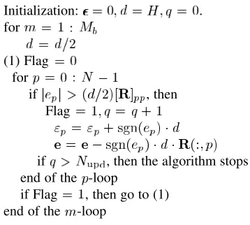
The system of equations to be solved is , where, for clarity, we have omitted the lower index associated with the sample period. For the solution of the system, the DCD algo-rithm [6] is used. The algoalgo-rithm is based on binary representa-tion of elements of the solurepresenta-tion vector with bits within an amplitude range . It starts an iterative approximation of the solution vector from the most significant bit. Once the most significant bit has been found for all vector elements, the algorithm starts updating the next less significant bit, and so on. If a bit update happens (such an iteration is called “successful”), the vector is also updated. The complexity of the algorithm is mainly due to “successful” iterations. To limit the complexity
(with an uncertain error of the solution), a limit for the number of “successful” iterations is predefined. If there is no such limit or the parameter is high enough, the accuracy of the solution is . Thus, parameters of the DCD algorithm are as follows: —number of bits used for representation of elements of the vector within an amplitude range
and —the maximum number of “successful” iterations, at which the solution vector is updated. Denote and elements of vectors and , respectively. The DCD algorithm can be im-plemented as follows.
Initialization: .
for
(1) Flag for
if , then
Flag
if , then the algorithm stops end of the -loop
if Flag , then go to (1) end of the -loop
The DCD algorithm guarantees convergence to the true solu-tion if elements of the true solusolu-tion vector are within the in-terval . It is seen from the algorithm description that if is a power of two, then multiplications by factors of power of two are only used; these can be replaced by bit shifts. Thus, the DCD algorithm can be implemented without explicit multipli-cations and divisions, which are well known to require a signifi-cantly higher chip area and power consumption in hardware im-plementation than addition and bit-shift operations. Moreover, divisions are often the source of numerical instability. The com-plexity of the DCD algorithm for a particular system of equa-tions depends on many factors. However, for given and , the peak (worst-case scenario) complexity can be shown to be
SACs (9)
IV. NUMERICALRESULTS
Now, we consider acoustic echo cancellation in the following scenario. The room acoustic impulse response has a length
[image:3.594.306.485.197.358.2]. The excitation signal is speech sampled at the frequency 8 kHz with a 16-bit resolution. In all FAP algorithms, the affine projection order is , and the step size is . The parameters of the DCD algorithm are set to and , while the number of updates , which controls the algorithm complexity and solution accuracy, is varying.
Fig. 1. Comparison of the misalignment (dB) for the ideal FAP, GS-FAP, and DCD-FAP algorithms.N = 8; = 1=8;SNR= 30dB.
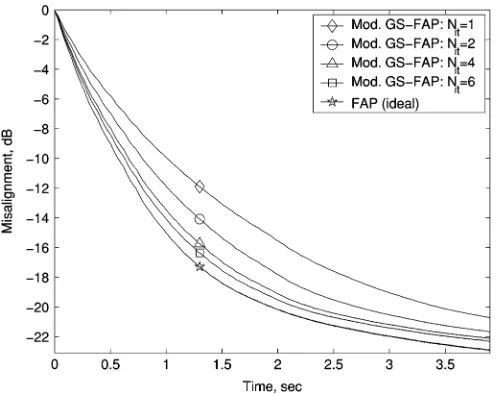
Fig. 2. Comparison of the misalignment (dB) for the ideal FAP and modified GS-FAP algorithms.N = 8; = 1=8;SNR= 30dB.
, the DCD-FAP algorithm provides a significantly better performance than the NLMS and GS-FAP algorithms. The performance of the DCD-FAP algorithm improves as increases, and for , it is close to the performance of the ideal FAP algorithm. Simulations for dB (not shown here) have demonstrated that “successful” updates provide nearly the same performance as the ideal FAP algorithm.
[image:4.594.40.289.312.509.2]Note that GS iterations can also be used to solve the system of equations in (6); we call such a combined algorithm the mod-ified GS-FAP algorithm. In this case, the number of iterations may need to be more than one. Fig. 2 shows how the perfor-mance of the modified GS-FAP algorithm is improved with the number of GS iterations and approaches that of the ideal FAP algorithm in the same scenario as in Fig. 1. It is seen that the modified GS-FAP algorithm with one iteration provides a better performance than the GS-FAP algorithm and approximately the
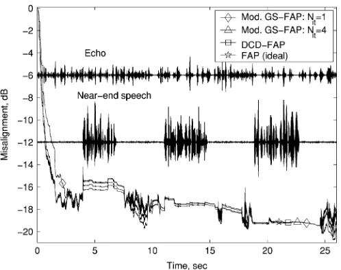
Fig. 3. Comparison of the misalignment (dB) for the ideal FAP, DCD-FAP
(N = 32), and modified GS-FAP (N = 1 and N = 4) algorithms with time-varying regularization in a double-talk scenario.
N = 8; = 1=8;SNR= 30dB.
same as the DCD-FAP algorithm with one “successful” update (see Fig. 1). For , we obtain a performance close to that of the ideal FAP algorithm.
In noisy conditions, especially in double-talk scenarios, regularization is a necessary part of adaptive algorithms. The adaptation should be slowed down in the presence of intensive near-end signals. Fig. 3 compares the misalignment for the ideal FAP, DCD-FAP and modified GS-FAP (
and ) algorithms in a double-talk scenario. In this sce-nario, the echo power is 11 dB below the near-end speech and SNR dB. The regularization parameter varies according to a simple technique based on approaches described in [5]
and [7]: , where
if or otherwise, , and
and are time-averaged powers of signals and , respectively. For averaging, attack-release filters were used with instantaneous attack and a slow-release time constant of 1 s, as in [5]. It is seen that the ideal FAP and DCD-FAP algorithms demonstrate performance with the misalignment difference being less than 1 dB. The modified GS-FAP algo-rithm with shows poorer performance, especially at the initial stage of the adaptation. For , its performance approaches that of the DCD-FAP algorithm with . Note that with , the performance of the DCD-FAP algorithm (not shown here) is the same as that of the modified GS-FAP algorithm with . The overall echo attenua-tion (ERLE) over the time interval between the 2nd and 26th seconds is approximately 17 dB for all three algorithms.
356 IEEE SIGNAL PROCESSING LETTERS, VOL. 12, NO. 5, MAY 2005
Fig. 4. Comparison of the misalignment (dB) for the ideal FAP, DCD-FAP
(N = 32), and modified GS-FAP (N = 1 and N = 4) algorithms with time-varying regularization in a double-talk scenario.
N = 8; = 1=8;SNR= 20dB.
In all trials, the complexity of the DCD algorithm for
, and 32 has not exceeded 128, 248, and 568 SACs, respec-tively. These are close to the peak DCD complexity from (9): 144, 256, and 592 SACs, respectively. The average complexity has been smaller: 75, 166, and 452 SACs, respectively. Simula-tions with smaller down to (not shown here) pro-duced a performance close to that for . As the peak DCD complexity depends mainly on , its reduction, in the case of , has not been significant (88, 200, and 472 SACs, respectively), but the average complexity has been re-duced greatly (67, 114, and 135 SACs, respectively).
For step (6), the modified GS-FAP algorithm requires approx-imately MACs and divisions; for and , this results in 256 MACs and 32 divisions. For the same performance, the DCD-FAP algorithm requires a maximum of 256 SACs and no multiplication or division. Note that, in our example, steps (3) and (8) of the adaptive filtering require ap-proximately MACs per sample, which is
signifi-cantly greater than the DCD peak complexity. MAC and divi-sion operations required for GS iterations are well known to be more complicated for hardware implementation than addition and bit-shift operations required for DCD iterations. Moreover, division operations are a source of numerical instability, and it is preferable to avoid them in real-time systems.
V. CONCLUSION
We have proposed a new approach for real-time implementa-tion of the fast affine projecimplementa-tion algorithm. This is based on the application of the dichotomous coordinate descent iterations for solving systems of linear equations in the FAP algorithm. As the DCD algorithm does not require explicit multiplications and divisions, it is well suited for implementation on real-time hardware and fixed-point software platforms, providing a com-putationally stable DCD-FAP algorithm. We have compared the performance of the new algorithm with the ideal FAP and Gauss–Seidel FAP algorithms in application to acoustic echo cancellation. It has been shown that the DCD-FAP algorithm demonstrates performance close to that of the ideal FAP algo-rithm and the complexity smaller than that of the Gauss–Seidel FAP algorithms.
REFERENCES
[1] A. H. Sayed,Fundamentals of Adaptive Filtering. New York: Wiley, 2003.
[2] S. L. Gay and S. Tavathia, “The fast affine projection algorithm,” inProc. ICASSP, 1995, pp. 3023–3026.
[3] H. Ding, “Stable Adaptive Filter and Method,” Int. Patent Application WO 0038319, Jun. 29, 2000.
[4] F. Albu, J. Kadlec, N. Coleman, and A. Fagan, “The Gauss-Seidel fast affine projection algorithm,” inProc. SIPS, San Diego, CA, Oct. 2002, pp. 109–114.
[5] E. Chau, H. Sheikhzadeh, and R. L. Brennan, “Complexity reduction and regularization of a fast affine projection algorithm for oversampled sub-band adaptive filters,” inProc. ICASSP, vol. 5, Montreal, QC, Canada, May 2004, pp. 109–112.