Image reconstruction using Wiener filtering and unsharp masking: a computer model

Rochester Institute of Technology

RIT Scholar Works

Theses Thesis/Dissertation Collections

7-1-1985

Image reconstruction using Wiener filtering and

unsharp masking: a computer model

Jay Berman

Follow this and additional works at:http://scholarworks.rit.edu/theses

This Thesis is brought to you for free and open access by the Thesis/Dissertation Collections at RIT Scholar Works. It has been accepted for inclusion in Theses by an authorized administrator of RIT Scholar Works. For more information, please [email protected].

Recommended Citation

IMAGE RECONSTRUCTION USING WIENER FILTERING AND

UN SHARP MASKING: A COMPUTER MODEL

By

Jay H. Berman

B.S. North Carolina State University

(1979)

A thesis presented in partial fulfillment

of the requirements for the degree of

Master of Science in the School of

Photographic Arts and Science in the

College of Graphic Arts and Photography

of the Rochester Institute of Technology

July, 1985

Signature of the Author

Jay H. Berman

Center for Imaging Science

Ronald Francis

COLLEGE OF GRAPHIC ARTS AND PHOTOGRAPHY

Rochester Institute of Technology

Rochester, New York

CERTIFICATE OF APPROVAL

M.S. DEGREE THESIS

The M.S. Degree Thesis of Jay H. Berman has been examined and approved by

the thesis committee as satisfactory for the thesis requirements for the Master of Science Degree

Edward Granger

Dr. Edward M. Granger, Thesis Advisor

Willem Brouwer

THESIS RELEASE PERMISSION FORM

ROCHESTER INSTITUTE OF TECHNOLOGY

COLLEGE OF GRAPHIC ARTS AND PHOTOGRAPHY

Title of Thesis: IMAGE RECONSTRUCTION USING WIENER FILTERING

AND UNSHARP MASKING: A COMPUTER MODEL

I, Jay H. Berman, hereby grant permission to the Wallace

Library of R.I.T. to reproduce my thesis in whole or in

part. Any reproduction will not be for commercial use or

profit.

IMAGE RECONSTRUCTION USING WIENER FILTERING AND

UNSHARP MASKING: A COMPUTER MODEL

By

Jay H. Berman

Submitted to the Center for _Imaging Science

in partial fulfillment of the requirements for the Master of Science degree at the Rochester Institute

of Technology.

ABSTRACT

Research was conducted to computer model and compare

the image reconstruction obtainable _using Wiener _filtering

and _unsharp masking. Wiener _filtering and _{unsharp masking}

are techniques used to improve image _quality and interpretation. It was demonstrated that far greater image

restoration is obtained _by Wiener filter than _{by unsharp}

masking because unsharp masking, unlike Wiener _filtering, enhanced image noise _along with the edges. A user _friendly

computer _model, that _may be used as a tutorial aid for Image Science _{students, incorporating} Fast Fourier Transform _(FFT) techniques was designed. Graphics allow the user to follow

ACKNOWLEDGEMENTS

Assistance from the _following sources is _greatly

appreciated. Without the _help of these dedicated

professionals this work would not have been done.

Dr. Edward M. Granger of the Eastman Kodak Co. and

Professor at the Rochester Institute of _Technology, for

acting as _my thesis advisor and _primary instructor in

this _exciting new field of Digital Image Processing;

The Eastman Kodak Co. for _allowing me the use of their

facilities and for sharing their expertise;

Dr. W. Brouwer for _acting as a member of the thesis

committee, keeping me on _{my toes,} and _providing helpful

assistance; and

The United States Air Force Institute of _Technology

(contract no. f33600-76-a-7299) for _paying the bills

and _sending me to Graduate School.

-111-LIST OF FIGURES

Figure 1. The Comb Function.

Figure 2. Illustration of the Nyquist Frequency.

Figure 3. The Point Spread Function.

Figure 4. The Line Spread Function.

Figure 5. The Bartlet Window.

Figure 6. The _{Unsharp Masking} Technique.

Figure 7. An Illustration of Contrast Enhancement.

Figure 8. An Image Restoration Process.

Figure 9. _Simulating an _Imaging System.

Figure 10. _Simulating a Restoration System.

Figure 11. The Ideal System.

Figure 12. _Restoring a Noiseless Object. Wiener Filter.

Figure 13. _Restoring a _Noisy Object. Wiener Filter.

Figure 14. Linear Fit for Wiener Filter Noise Response.

Figure 15. Wiener Filter Restoration Response.

Figure 16. _{Restoring Noisy} Images. Wiener Filter.

Figure 17. _Restoring Blurred Images. Wiener Filter.

Figure 18. Restoring a Noiseless Object. _Unsharp Masking,

Figure 19. Restoring a Noiseless Object. _Masking Filter.

Figure 20. An Illustration of Contrast Enhancement.

Figure 21. Restoring a _Noisy Object. _Unsharp Masking.

Figure 22. Performance of the _{Unsharp Masking} Technique.

Figure 24. Restoring Blurred Images. _Unsharp Masking.

Figure 25. Noiseless Image Restoration. Wiener and Masking,

Figure 26. _Noisy Image Restoration. Wiener and Masking.

Figure 27. Comparison of Wiener Filter and _{Unsharp Masking}

Restoration Responses. ( Varying Noise).

Figure 28. Comparison of Wiener Filter and _{Unsharp Masking}

Restoration Responses. ( Varying Cutoff _Freq.)

Figure 29. _{Unsharp Masking} Approximation of the

Inverse Filter.

Figure 30. A Model for _Unsharp Masking.

-INTRODUCTION

The purpose of digital image _processing and enhancement

is to improve picture _quality or image interpretation. More

specifically, it is used to remove _noise, to enhance object's

edges, and to highlight specified features. (1). For the

photointerpreter, scientist, surgeon,and others who analyze

images, it is important to extract as much useful information

from an image as possible. Often much of this information is

contained in the fine detail of the image which is hard to

resolve because of noise and _blurring, Wiener _filtering and

unsharp masking are two image _processing techniques which

have been used to _help the user get at this information

and/or improve picture quality.

As is implied _by the name Digital Image _Processing,

images are processed _by computers _using discrete values

obtained _{by sampling} an actual image. _However, real images

are continuous. _Sampling implies that not _every member of a

population (in the case of _film, not _every silver crystal) is

measured. Therefore, how an image is sampled is critical to

the _study of Digital Image Processing. Discrete values taken

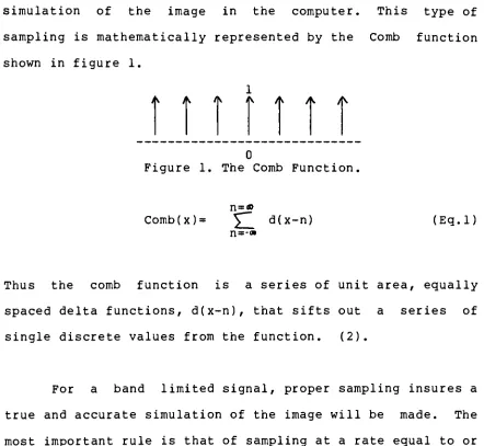
simulation of the image in the computer. This type of

sampling is mathematically represented _by the Comb function

shown in figure 1.

Figure 1. The Comb Function,

n=

Comb(x)=

^_

n=-(Eq.l)

Thus the comb function is a series of unit _{area, equally}

spaced delta _{functions, d(x-n),} that sifts out a series of

single discrete values from the function. (2).

For a band limited signal, proper _sampling insures a

true and accurate simulation of the image will be made. The

most important rule is that of _sampling at a rate equal to or

smaller than the interval AX calculated _by the Nyquist

criteria. The Nyquist criteria requires that the image be

sampled at a rate A X such that the highest _frequency of

interest Fn is given by:

Fn = _1/(2*X) Therefore: AX = _{l/2Fn (Eq.2,3)}

-In _any case where the signal is band limited within the

region of bandwidth Fn and AX = _{l/2Fn the function}

may be

reconstructed exactly.

Incorrect _sampling will cause aliasing, the _overlapping

of _displaced, adjacent _{spectra, making} exact image _recovery

impossible. (3) For this _reason, when _processing images _using

FFTs it is important to band limit and sample correctly. For

example, given a function with N=256 points and a Nyquist

frequency = _{128.0 lines/mm, what}

sampling interval (AX)

should be used? Figure 2 and the _following mathematics

provide a good guideline:

G(F)

-3Fn -2Fn -Fn 0 Fn 2Fn 3Fn

Figure 2. Illustration of the Nyquist frequency.

Fn = _1/(2MX) lines/mm _(Eq.4)

Thus: AX = 1/(2* _Fn) = _{1/(2*128) =1/256 mm}

(Eq.5)

Also: AF = Ft/256 = _256/256 = _{1 line/mm}

Figure 2 depicts the Discrete Fourier Transform G(F).

The function is band limited from -Fn to Fn in accordance

with the Nyquist criteria. The total _{frequency range, Ft,} is

from -Fn to Fn with N number of discrete points separated _by

F. _However, because of _sampling, Discrete Fourier Transforms

are periodic. The periodic nature of these functions

prevents the loss of information in _performing the inverse

transformation always associated with _sharp cutoffs in the

frequency domain.

The importance of _sampling can not be stressed enough.

Using the simple concepts just presented will insure the best

reconstruction of an image. Just as important as _sampling,

an _{understanding} of how light behaves and how optical systems

respond to produce an image is _primary to _determining the

type of image processing used. A short tutorial of these

factors is presented here.

The irreducible object element is the mathematical

point. A fundamental characteristic of _any photographic

material involves the way which a point or a line (an

assemblage of points) is imaged within the material. Due to

the nature of photographic _{emulsions, lenses,} and other

elements in an optical _system, the irradiance _{energy falling}

on a film from a point or line is to some degree diffused and

-spread within the emulsion. (4). For an image of a point or

a _line, this distribution of the irradiance _by the emulsion

is known as its point spread _{function, (p(x,y)),} and line

spread _(l(x)) function respectively. Figures 3 and 4 are

plots of the point and line spread functions.

Figure 3. The Point Spread Function,

The Fourier transform of _l(x) is _{(L(f)), commonly} known

as the Optical Transfer Function (OTF). The modulus of the

OTF is known as the Modulation Transfer Function (MTF). The

OTF and the MTF are _presently the most _widely used criteria

for _evaluating optical systems. The _following mathematics

illustrate the relationships of the functions just discussed:

(5,6)

Kx) =

jp(x,y)

re -i2TT fx

L(f)=/l(x)e dx = _{OTF(f) (Eq.8)}

MTF(f) = _{OTF(f) (Eq.9)}

NOTE: Throughout the rest of this _{paper, #^} will represent

the Fourier Transformation. Therefore, l(x) $*t L(f).

Another limitation associated with all films is

graininess. Due to the discrete nature of film grains and

because it is impossible to to make a _truly monodispersed

emulsion (an emulsion in which all of the _imaging particles

are the same size and are _{evenly dispersed),} noise results in

-the image. Noise is a general term used to refer to _any

undesired signal recorded on a _recording medium or picked _up

by an instrument designed to respond to a certain _signal; for

example, static on a television or a radio. Photosensitive

grains or small integral areas on an emulsion _receiving equal

exposures do not have equal densities when developed. These

fluctuations in _density are _commonly referred to as grain and

produce image noise. (7).

Image noise _(G) on a film is defined as the product of

the measured mean-squared _density fluctuations (T(a)**2 and

the area of the _scanning aperture _(A) used to make the

measurement. (8) .

G = _{A cr(a)**2} (Eq.10)

Image noise is related to _{granularity by} the following:

S =

a (a) J~TA (Eq.ll)

Thus: S**2 =(/2A CT (a) ) **2 = _{2G (Eq.12)}

Where ** indicates exponentiation, S is the Selwyn

granularity coefficient, and _(7(a) is the root-mean-square

The combination of the optics and _film, and the grain

of the film _usually degrade the object _being photographed.

These undesirable effects are _easily seen in aerial

reconnaissance where the objects of interest often appear as

very blurred and _grainy images on the film. To improve the

image, or in this _case, make it more like the original scene,

enhancements filters are used to reduce image noise and to

sharpen faint or _barely recognizable details from blurred

edges. This report will compare two enhancement _techniques,

Wiener _filtering and _unsharp masking.

The Wiener filter is a mathematical algorithm designed

to enhance images _by removing noise and _sharpening edges. Its

design is governed _by a prior knowledge of the noise in the

system. The _following is the mathematical description of the

Wiener filter (11,12)

H

* _{2 2 2}

(f) = _{L (f)} /

[L(f)

)]

Where L*(f) denotes the complex conjugate of _L(f), normalized

to _L(0)=1, and N (f) and 0 _(f) are the noise and input signal

power spectra.

-By examining equation 13 it is _easy to see how the

Wiener filter works. When the noise power _greatly exceeds

the input signal _power, which happens at _very high

frequencies, H(f)--_{>0; the filter allows}

very little signal

to pass through it. If the signal is much greater than

noise, as happens to be the case for the lower _frequencies,

H(f)~> L *

(fJ/LU)1

= _{1/L(f) thus}

allowing most signals to

pass through the filter. For noiseless conditions the Wiener

filter becomes an inverse filter. For signal/noise ratios in

between these extremes the Wiener filter responds

accordingly. (13,14). Even though some of the noise will be

passed _by the filter and some of the signal _lost, the Wiener

filter is considered the optimal restoration filter in a

least squares sense and the standard to which other _filtering

techniques are compared to because it minimizes the

mean-square differences between the input and the restored

target. (15,16).

The noise power (Wiener) spectrum of an image is the

Fourier decomposition of the noise. It can be used in the

frequency domain as a statistical evaluation of image noise.

(17,18,19,20). Once an estimate of the noise Wiener spectrum

designed. The several steps which must be taken to estimate

the Wiener spectrum are outlined below:

First calculate the mean _density or signal in the system and

subtract this mean value from each data point. These values fluctuating about the mean are the noise. The next _step is

to perform the technique of noise windowing. To better describe this technique the triangular or Bartlet window is

described below. Figure 5 illustrates the technique _using the Bartlet window (21).

RRNDOtt GRUSSIRN NOISE NOISE WINDOW FILTER W(X) _{WINDOWED GRUSSIRN NOISE} 3.

a*

h

is

b

Figure 5: The Bartlet Window.

/ 1

-|2x/c|

w(x) = <

V 0 elsewher

x| C/2

(Eq.14)

-C. fsin ( Cf/2)1 C 2

= ₂

L

J

w(x)4==7W(f) = ₂ L _f/2 J = _{2 sine (Cf/2) (Eq.15)}

The _windowing is performed _{by multiplying} the noise data

(n(x)) with the window w(x). As is apparent the window acts to limit the extent of the _noise, and it also eliminates end

transitions that cause Wiener spectrum estimate error that

could occur when _performing the third _step, FFT the windowed

noise. These three steps yield the _following advantages:

1) Eliminates discontinuities at the end of data files. 2) Prevents _wrap around when _estimating Wiener Spectrum

by using an FFT algorithm.

3) Smooths the power spectrum. (Note: Multiplication in the space domain is a convolution in the _frequency

domain. ) (22) .

Once the windowed noise is _found, it is transformed to the

frequency domain. This is used in the final step. The final

The Wiener spectrum just calculated is used in Eq.13 to

produce the optimal Wiener filter. The noise _reducing

characteristic of the Wiener filter is not present in the

unsharp masking technique. As previously indicated this is

the second filter that will be examined.

The _{unsharp masking} technique aids in the retention of

detail and improves the visual appearance of an image _by

sharpening the edges between distinct objects in the image _by

exaggerating the _density difference across the edge. (23).

Yule _(24,25) outlines the procedure for _implementing the

unsharp mask technique. An _unsharp mask of an original scene

is produced on a _moderately low contrast film (contrast

compression). The mask image is opposite in sign from the

original. This _may be achieved _by contact _printing the

original and the mask with a sheet of diffusion material

between them or _{by defocusing} if _using a projection system.

The original and the mask are combined in register and used

to produce a final image on a higher contrast _material; the

higher contrast material compensates for the contrast

reduction _resulting from the combination of the original and

the mask.

-The _unsharp mask affects the final image _{by reducing}

the large scale tonal differences or _density ranges of the

low frequencies. The fine details are blurred _by the _unsharp

mask. When the final image is made _using the original image

and mask the contrast differences of the fine details are

maintained because _they are not _drastically effected _by the

subtraction. This results in an increased contrast

difference along an edge gradient (improved sharpness) when

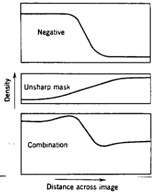
the original contrast is restored. (26). Figure 6 is an

illustration of the _{unsharp masking} technique. Note the

increased _density range due to the _hump and _{dip along} the

edge gradient _resulting from the _unsharp mask.

Negative

Distanceacrossimage

Actionof_unsharpmaskin_improvingedgesharpness.

The _unsharp mask combined with the degraded image _may

be regarded as a filter in the _frequency domain with its OTF

increasing with spatial frequency. This results in an

increase in output modulation and MTF values greater than

unity, the phenomenon of contrast enhancement (28,29).

Figure 7 is an illustration of contrast enhancement from a

filter with a negative spread function.

itr

vf

SIMULATED FILM MTF

10' 10" swift, ftieouijcy

MASK TRANSFER FUNCTION

10' 10* rmin. ncnuoer

SYSTEM MTF (CONTRAST ENHANCEMENT)

10"

10"

10"

10' io1 smt1h. fhoucj

10"

Figure 7. An Illustration of Contrast Enhancement,

-From figure _7, observe that the _unsharp mask, used here

in the technique of contrast enhancement acts as a

restoration filter and in its theoretical ideal case

approximates an inverse filter. Two questions arise from

this illustration: ₁₎ How do we determine the line spread

function used to create the desired _unsharp mask? 2) Once

the _{unsharp masking} technique is _modeled, how can it be

described it in terms of modulation transfer theory? The

following discussion will answer these question.

To create the desired _unsharp mask and achieve the best

object restoration through contrast _enhancement, it is

necessary to look at the mathematics involved. The _following

mathematics, utilizes Fourier techniques in the _frequency

domain, were developed _by E.M. Granger (30,31). This work

follows a line of thought similar to _{Armitage, Lohmann,} and

Herrick (32) with the added advantages of _yielding an optimum

restored image in a least squared _sense, and it is not

subject to the contrast limitations specified in the

The _following symbolism will be used:

0(F) = _{OBJECT Bl} = _CONSTANT

MTF(F) = FILM1 B2 = CONSTANT

KF) = _{IMAGE Gl} = _{FILM GAMMA IMAGE}

U(F) = _{FILM2 G2} = _{FILM GAMMA MASK}

MASK(F) = _{MASK G3} = _{FILM GAMMA FINAL}

M2 = _{2ND MOMENT PI} = _3.14159

RO(F) = _{RESTORED OBJECT}

0(F) * MTF(F) = _{1(F) 1(F)} * _U(F) = _{MASK(F) (Eq.16,17)}

Solving simultaneously;

MASK(F) = _0(F) * _MTF<F) * _{U(F) (Eq.18)}

Note that both _MASK(F) and _U(F) are unknown.

Therefore, to solve for _MASK(F), U(F) must be written in a

non-variable form. A _way to do this is extracted from the

Second Moment Technique developed _by E.M. Granger (33). This

technique provides a means of _estimating the MTF of a

system/element in a system _by the statistical second moment

of the l(x). It is used here to determine the _{l(x) necessary}

to produce the _unsharp mask. He found the _following

relationship exists:

-2 2 MTF = ₁

-(2pi F M2) M2 is the Second Moment. (Eq.19)

For the complete derivation see the reference.

Substituting the Second Moment Approximation for _MTF(F) and

U(F) into equations 16 and 17:

2 2

I(F)=0(F)*(l-(2pi *M2*F )) and _(Eq.20)

2 2

MASK(F)=I(F)*(l-(2pi *M2*F )) (Eq.21)

Therefore:

2 2

I(F)=0(F)*(1-(B1 * _{F )) where Bl=2pi *M2 and}

(Eq.22)

2 2

MASK(F)=I(F)*(1-(B2 * _{F )) where B2=2pi *M2}

(Eq.23)

From Eq.18 or _{by combining Eq.22,}23:

2 2

MASK(F) = _0(F) * _(1-(B1 * _{F ))} * (1-(B2 * _{F )) (Eq.24)}

2 J> 4

MASK(F) = _0(F) * (1-(B1+B2) * F ) + (Bl*B2/* F ) (Eq.25) IKO.T.

The next _step in restoring the original object is to combine

the image and the mask in register and exposed them onto a

higher gamma film. The following mathematics illustrate

RO(F) = _(I(F)+

MASK(F)) _(Eq.26)

Substitute _Eq.22,25 into 26. Include film gamma constants.

2 RO(F)= G3* _{( (G1*0(F)*(1-B1*F}

)) +

2

(G2*0(F)*(1-(B1+B2)*F )) (Eq.27)

2 2

=

G3( (G1*0(F)-(G1*0(F)*B1*F ) + _(G2*0(F)

-(G2*0(F)*Bl*F )

-2

(G2*0(F)*B2*F ) (Eq.28)

RO(F) = _{G3*( (G1+G2)*0(F)}

-2 2

(G1+G2)*0(F)*B1*F -G2*0(F)*B2*F ) (Eq.29)

=

G3*nGl+G2)*0(F)-0(F)*(

))

RO(F) = _G3 * _0(F)

(

-2 x ( (G1+G2)*B1 + G2*B2 ₎ *F

J

To obtain optimum enhancement set _(G1+G2) * _{Bl + G2} * B2 2

equal to zero and thus eliminate the F dependence.

Therefore: Gl*Bl =

-G2*(B1+B2) (Eq.32)

image mask

-G1/G2 = (Bl+B2)/Bl (Eq.33)

-Observe that the mask and image are opposite in contrast.

To restore original contrast chose values so that:

G3 * _(G1+G2) = _{1.0 (Eq.34)}

The derivation above allows for direct _modeling of the

unsharp mask. To describe the _{unsharp masking} technique as a

linear filter in terms of modulation transfer _theory the

operation involved must be _{approximately} linear. The

mathematical linear approximation for _masking, developed _by

Armitage, Lohmann, and Herrick ₍₃₄₎ is:

Tr(s) = Gl- _{G2(m)*Tr(m) (Eq.35)}

where Tr(s) is the system MTF (MTF of the final _image), G2(m)

is the mask contrast, and Tr(m) is the MTF of the mask.

Incorporating the results of the Granger method into their

approach allows the _{unsharp masking} technique to be expressed

in terms of a linear filter, free of small contrast

limitations, and allows the final MTF of the _masking

technique to be _easily calculated. For the complete

formula it is apparent that Tr(m) must be negative to yield a

final MTF of 1.0.

As _previously illustrated (Figure _{6), unsharp masking} enhances edges _{by adding} the original image with a blurred negative of the original in register. Therefore, any spread

function and or film contrast combination _may be chosen to

create the mask. _However, this _may not optimum if the

combination is not chosen _according to the rules provided in

equations 16-34. Other contrast values and spread function

combinations will result in varied degrees of edge

enhancement.

According to Scarff, (35) unsharp masking results in

more _visually pleasing photographs if the images are not made

to sharp. In his experiments he learned that a final image

with a maximum MTF of 1.3 produced from a scene with an input

modulation of .70 was visually preferred over the same an

image of the same scene produced at a higher or lower MTF.

However, he does not draw _any conclusions about images

produced from scenes with other input modulations or the

effects of S/N on image quality.

-OBJECTIVES

It is the objective of this research to determine to

what degree of image restoration is possible, what are the

limitations to image enhancement/restoration _using these two

techniques, and how do these filters differ. This paper will

quantify, analyze, and compare the digital image _processing

techniques of Wiener _filtering and _unsharp masking. To _study

these _methods, noise and image components are _cascaded, in

the _frequency domain _using Fast Fourier _Transforms, through a

series of mathematical filters and transfer functions. The

model allows the user to examine each stage of the

processing. It is expected that a greater degree of image

reconstruction _{(restoration)} is obtainable with the Wiener

filter than with the _unsharp mask.

Another objective of this work is to design a user

oriented computer model that will aid students in _learning

and understanding the use of Fourier Transform Techniques for

EXPERIMENTAL

The experimental part of this research consisted of

writing an image _processing computer model and an analysis of

data obtained from the model. The experimental model was

designed in FORTRAN on an IBM/CMS computer system. The model

can _easily be incorporated into _any system that supports

FORTRAN 77 and the IMSL Library. The IMSL _Library is a set of

statistical and scientific FORTRAN programs available on _many

main frame computers. All graphics generated _by this model

were made _using the 'DISSPLA*

software package. 'DISSPLA' is

a product of the Integrated Software Systems _Corporation, San

Diego, California 92121. The IBM system was used because of

availability, speed, and the vast amount of scientific

software _supporting it.

The image processing model used has a modular design to

provide flexibility, ease for the _user, and a tool for

learning. The modular design allows the user to choose

predefined elements or substitute a simulation into the

process. Various combinations were used and analyzed by this

researcher with the major goal to obtain optimal

reconstruction from the various inputted specifications.

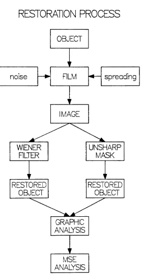
Figure 8 is an illustration of the image restoration process.

RESTORATION PROCESS

WIENER FILTER

RESTORED

OBJECT

OBJECT

spreading

IMAGE

UNSHARP MASK

RESTORED

OBJECT

GRAPHIC ANALYSIS

MSE ANALYSIS

Each process illustrated here is software supported.

Documentation for and a _copy of each experimental program

used is provided in the Appendix.

Discrete FFT techniques were incorporated into the

modular design. It is _{faster, easier,} and less expensive to

do this digital image _processing in the _frequency domain by

cascading (multiplying) frequency components than in the

spatial domain via convolution. A 256 point FFT was chosen

to reduce _processing time and because of limited computer

memory allocation. _Using 256 points imposes a limitation on

the model; the transform of a bounded function in the spatial

domain is _{theoretically} unbounded in the _frequency domain.

Cutting off a function results in the loss of information at

the higher frequencies beyond the cutoff frequency. _However,

as discussed in the _{Introduction,} the Discrete FFT prevents

the loss of information because of its periodic _nature; the

function in the spatial domain is _exactly recovered _by

inverse transforming. Despite these limitations both

frequency and spatial domains can be well represented with

256 points. For the 256 points, a _frequency range of -160 to

160 cycles per millimeter (cyc/mm) was chosen because _many

films can be modeled well over this range. _Using the

mathematics discussed in the Introduction on sampling theory,

-we calculate AF=1.25 _cyc/mm, AX= _1/320

mm, and the spatial

range from -.40mm to .40mm.

As illustrated on figure _8, the first _step in the

restoration process is to simulate an object. A 5cyc/mm

tribar target was chosen for this work. _Using this simple

target for the object has the _following advantages:

1) It is a _widely used standard in image _processing and

evaluation.

2) Each cycle has 64 data points for analysis.

3) It is _easy to see and examine the degradation and

restoration _graphically as the image passes through the

system.

4) Tribar targets are _easy to analyze mathematically.

The next _step in the model is to degrade the object

using a simulated film model. This is done _{by blurring} the

object and _adding random gaussian noise to _it, thus _yielding

a simulated film image. The object was blurred _by

multiplying it in the frequency domain with an MTF curve

generated _using the widely accepted Frieser model. The

Frieser model is defined as:

2

where f is _frequency and <X is the parameter _controlling the

width of the curve. Note that the MTF for the Frieser model

does not go to 0. For this _case, the periodic nature of the

Discrete FFT is _especially important in _preventing the loss

of information when _performing digital image processing. To

simulate the random _density fluctuations found in exposed

film, random numbers from a gaussian distribution with a mean

of zero and a user defined variance are then added to the

blurred image.

As shown in figure _8, the next _step in the restoration

process is to reconstruct the tribar object via the Wiener

Filtering and _{Unsharp Masking} techniques. This _step in the

simulation is the thrust of this research. The results of

these two techniques will be _{analyzed, compared,} and

quantified in the results section of this thesis. The

mathematics involved in these restorations have been

thoroughly described in the Introduction and are used in the

computer model.

The final _step in the computer simulation is the

generation of data and graphics from these two restoration

methods. Two types of analysis will be performed; a graphics

analysis which allows us to see a graphical representation of

-every phase of the restoration process for the two _filters

and a mathematical analysis of the mean-square error of the

restored object compared to the original. The graphic

simulations generated _by the model permits a visual

comparison of the two techniques. The data collected _by the

mathematical technique is used to generate graphs _showing the

degree of image restoration and behavior of the filters for

various levels of _degradation. The data and graphs collected

RESULTS

This research has found the Wiener _filtering technique

to be superior to the _{unsharp masking} technique for image

restoration under all test conditions within the limits of

the image _processing model developed for this work. The

results that will be presented in this section will show this

quantitatively and graphically. Before _any data could be

collected, a digital image _processing model to simulate the

unsharp masking and Wiener _filtering techniques was

developed. The model allows the user to examine each stage

of the simulation process graphically.

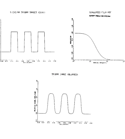
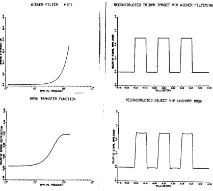
Figures 9 and 10 shows the simulation developed for

this research. Illustrated here are some of the major

imaging elements and _processing stages simulated _by the

model. Figure 9 (from _top left) simulates a 5cyc/mm tribar object _being blurred by a hypothetical film with an MTF

cutoff of lOOcyc/mm under noiseless conditions to yield an

image. As is easily seen this results in an image of the

object that is blurred and rounded off _{particularly along} the

edges. Figure 10 shows the object restoration attainable

with the Wiener filter and the _unsharp mask.

-5 CYC/MM TRIBAR TARGET (0(X1) SIMULATED FILM MTF ajicrr run- xx> ctc/uu

h--o.w -o.v u.v n* in" in'

spfiTim nro*trjr i

TRIBAR IMAGE (BLURRED)

i

xtf

WIENER FILTER HIF)

10' 10" SfflTld. nEOUDCT

MRSK TRANSFER FUNCTION

10"

RECONSTRUCTED TRIBRR TARGET VIA WIENER FILTERING

3

I

i

V)

RECONSTRUCTED OBJECT VIA UNSHARP MASK

10* 10" I0" 10"

i

1

J

-. *cjb *_* -___i +m ijs o.a t.M waiicTots

Figure 10. _Simulating a Restoration System,

-It was _{mathematically} shown in the introduction that

under _{theoretically} noiseless conditions the Wiener filter

was an inverse filter. _Using an inverse filter to restore a

noiseless image yields a perfect reconstruction of the object

if the simulation does not suffer from the effects of _sharp

cutoffs. Because the Freiser model does not go to 0, all 256

points are used in both the spatial and _{frequency domains,}

and due to the periodic nature of Discrete FFTs, the

simulation created for this research does not exhibit _sharp

cutoffs. The graph of the restored object demonstrates this

perfect restoration _using Wiener filtering. Also shown in

the _{Introduction,} figure 6, was that a smooth image combined

with a _smooth, blurred mask resulted in a sharper image with

exaggerated edges. These _results, shown in figure _10, for a

noiseless system agree with the results expected from theory.

As was stated in the _objectives, the data collected

will be use to quantify, analyze, and compare the two

techniques. Data collected _separately allows each method to

be quantified and analyzed individually. The _information,

results, and data gathered _separately will be included with

data obtained collectively to permit a thorough comparison of

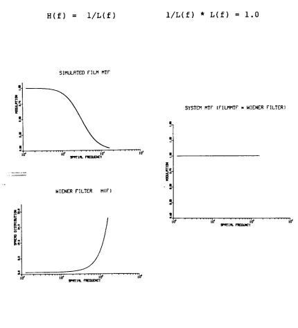
The Wiener filter will be looked at first. Note in

figure 11, since the film does not go to _0, neither will the

Wiener filter or the final MTF. The Wiener filter yields

perfect restoration of the object in the absence of noise

regardless of the spread function _degrading the image. This

is possible because the Wiener filter becomes the inverse of

the film spread function so the effective system MTF over the

entire _frequency range simulated is _1.0, an ideal system.

This is illustrated _by the _following equation and graph in

figure 11:

-H(f) = _1/L(f) 1/L(f) * L(f) = _1.0

SIMULATED FILM MTF

SYSTEM MTF (FILMMTF n WIENER FILTER)

10*

jpmin. nsnuDCT

WIENER FILTER HIF)

itf

10* 10" 10* 9nniL nsoicr

10*

10* _iff "J1

jpmid. neouocr

io"

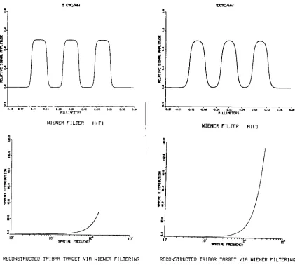
Figure 12 show the reconstructions of a 5cyc/mm object

(left side) and a lOcyc/mm object (right side) blurred _by a

film with a cutoff _frequency of 150cyc/mm _using Wiener

Filtering. The lOcyc/mm restored object is 2X scaled to

provide ease in _comparing the two restorations. Note perfect

restoration in both cases is achieved even though the

lOcyc/mm image is more degraded. Also _note, that the filter

for the more degraded image rises much faster.

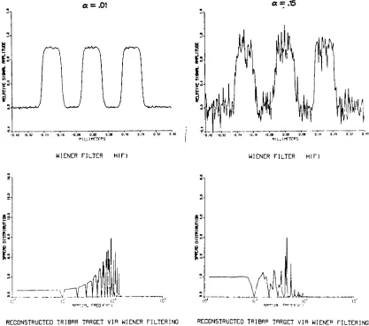
In the presence of noise the Wiener filter responds

differently. As indicated in the _{introduction,} the filter

seeks a compromise between noise removal and edge _sharpening

dependent on the degree of the degradation due to each

factor. To determine the filter's overall response to

varying noise a series of restorations runs were performed

and analyzed. Figure 13 illustrates two of these runs.

Shown are the images of a 5cyc/mm target degraded _by a film

with a cutoff frequency of 150cyc/mm Alpha noise level of .01

(left side, low noise) and .15 (right side, high noise). For

the case of the low noise, high S/N, note the edges are

enhanced but at the expense of _increasing the noise. For the

high noise case, low S/N, much of the noise is removed but

little is done to sharpen edges. Also _note, the filter for

the lower noise case rise three times faster.

-TRIBAR IMAGE (BLURRED)

SCYC/UJ

WIENER FILTER HIF)

Sg

is

C_g o e u

10" 10' 10"

SPflTIft. FUEOUOCY

101

TRIBAR IMAGE (BLURRED)

CCrC/Ui

WIENER FILTER HIF)

Es-I

l(f if "itr" surin. ncouocr

ID-RECONSTRUCTED TPIBAR TARGET VIA WIENER FILTERING RECONSTRUCTED TRIBAR TARGET VIA WIENER FILTERING

-C.1D -0.3"

-C.21 .16 -C.0B 0.0C COP 11.16 O.W 0.17 0.1

h

i

-0. -C.l <A2 -tJM -0.04 D.OD 0.01 O.OB 0.11 O.IS D.3D

MLLITCTEFS

NOISY BLURRED TRIBAR IMAGE

a=.01

NOISY BLURRED TRIBAR IMAGE

a=.15

w

#1

yf

\j

f\

033 C. ___, hj.s; -CM -C.,* -o.OS O.OC O.OB D.lfi C* T.l?

| MiL^mrTrPS

WIENER FILTER HIF) WIENER FILTER HIF)

w::\_tpeo

11...T_

s: i

D e I:

u

w

s^TIfl rorn-tirr

RECONSTRUCTED TRIBAR TARGET VIR WIENER FILTERING RECONSTRUCTED TRIBAP TARGET VIA WIENE* _FILTERING

t

aAAH

v^pvwwj wvA-^

tWvW W*^^

/VvVA^J VV^A/Wv

-040 -03? 0"M 0.16 -o. t.OO 0.0" O.IB 0.3* o.s? o 10 -010 -0.3? -C?* -C ?i r.i? c.ic

Figure 13. Restoring a _Noisy Object. Wiener filter

-This brought _up an _interesting question: At what point

does the filter respond more like a noise removal filter and

less like an inverse (edge enhancement) filter? figure 14

answers this question. It shows one result of this series of

restoration runs. It is a graph _showing S/N (in) vs S/N (out)

of the system. It shows for S/N(in) less than 40:1 the

filter reduces noise and for S/N(in) greater than 40:1 it

will sacrifice _(increase) the noise in favor of _enhancing the

edges. The data on figure 14 appears to fit a Y=aX**b curve.

If this is _so, it will plot as a straight line on a _log-log

graph and the Wiener filter's performance _may be qualified.

The fit is good statistically. _Using a T _test, it falls

well within the 95% confidence limits for S/N(in) ratios

999.99

COMPARISON OF WIENER FILTERING TO UNEAR RT

S/N

(in)

(out)

S/N after filtering

100

10-

->-...!-""r"i-"!"!-:-t

.^... ...

....-..<.-.-...;...

O WIENER FILTERING

D UNEAR FIT

>:>.-:

.. ...

<---:~i--f>

/

i

i

i

/Mi!

10 100

S/N before

filtering

1000

Figure 14. Linear Fit for Wiener Filter Noise Response

-Figure 14 leads an observer to wonder if there are

circumstances that will result in a restored object that is

worse than the image before filtering. In other _words, can

the noise degradation become so great as to cancel out the

improvements of the edge enhancement? Figure 15 is a plot of

the standard error for the image before restoration vs the

standard error for the restored object at various levels of

degradation, where:

Standard Error =/_> [Restored _Image

-Object] / n _(Eq.42)

It shows that the Wiener filter always yields an improvement

regardless of the error _resulting from the noise and cutoff

WIENER FILTER RESTORATION

STANDARD

ERROR(out)

ERROR(ln)

Standard Error after_filtering

0.12

0.10-

0.08-

0.06-0.04

0.05 0.10 0.15 0.20 0.25

Standard Error before

Filtering

0.30

Figure 15. Wiener Filter Restoration Response

-Figure 16 shows how much improvement is made. Observe

that _doubling the noise does not result in a restored object

with twice the restoration _error, as some might expect.

Instead, a greater proportion of restoration is gained from a

noisier image than from an image that has less noise. This

is depicted _by the gradual _leveling off of the curves as the

noise _increases; the more noise there _is, the easier it is to

remove. A user can quite _accurately predict the degree of

restoration the model will yield from this graph.

Figure 17 is a graph of the same data used to create

figure 16 except cutoff _frequency is the independent variable

instead of noise. Observe that restoration error is

gradually increasing as cutoff _frequency decreases _(blurring

increasing). Because figure 17 shows greater curvature than

figure _16, restoration is more dependent on the degree of

WIENER FILTERING

CUTOFF FREQVS RESTORATION ERROR

STANDARDERROR

0.06

0.04

NOISE_LEVELfa)

Figure 16. _{Restoring Noisy} Images. Wiener Filter

WIENERFILTERING

RESTORATION ERROR VS CUTOFF FREQ.

STANDARDERROR

0.08

0.06

0.04-CUTOFF FREQUENCY

Figure 17. Restoring Blurred Images. Wiener Filter.

-The performance of the _unsharp mask will now be

analyzed. _{Unsharp masking} was simulated for an image on a

film of gamma = _{1.0, a mask of film gamma} =

.7, and the

restored object on to a film with gamma = _{3.334. Figure 18}

shows the reconstructions of a 5cyc/mm object (left side) and

a lOcyc/mm object (right side) degraded _by a film with a

cutoff _frequency of 150cyc/mm under noiseless conditions via

the direct _method, an image placed in register with the

unsharp mask, of _unsharp masking. Note the lOcyc/mm object

is 2X scaled to allow an easier comparison of the two

restorations. Observe a better restoration of a target is

attained from a less blurred image.

As just illustrated in the figure _{18, unsharp masking}

is _usually performed in the spatial domain. Since it went

from a blurred image to a sharper _image, the _{unsharp masking}

technique can be described in the frequency domain as a

linear transfer filter. Using the mathematics developed in

the Introduction, an approximation of a linear _filter, the

mask transfer _function, for the technique is attainable. This

is shown in figure 19. Observe in this figure that the same

restoration as is shown in figure 18 resulted. Because the

two methods yield identical results the model is not limited

TRIBAR IMAGE (BLURRED)

5CYCAM

TRIBAR IMAGE (BLURRED) 10CfCAM

UNSHARP MASK UNSHARP MASK

i

B.W -0.33 -C.M -*-IO -D.00 0.00 O.OB O.IB O.Ji 0.33 0. -0.30 -0.11 -.U -4.00 -0.04 O.OD 0.O4 0.01 0.12 0.10 O.X

tllLUtCTERS niu.ifinDts

RECONSTRUCTED OBJECT VIA UNSHARP MASK _{RECONSTRUCTED OBJECT VIA UNSHARP MASK}

i-U

r i

u

d _, , , , , 1 . _f^

, , <m <33 4.M -0-10 <-0> 0.OD 0.01 0.10 O.M 0.33 0- ____, -_.|t _._}

MILLIMZTEP5

Figure 18. Restoring a Noiseless Object. _Unsharp Masking,

-TRIBAR IMAGE (BLURRED)

sctcam

TRIBAR IMAGE (BLURRED)

tJCYC/WM

-. U -%M -.u

MASK TRANSFER FUNCTION _{MASK TRANSFER FUNCTION}

5

Id1

10' 10" swift,ncouocr

10"

e

i o

10* 10' 10*

SPRT1U.n___J_MCY

RECONSTRUCTED OBJECT VIA UNSHARP MASK RECONSTRUCTED OBJECT VIA UNSHARP MASK

s

b

i

j

u

u

rn

_. -ojj ** I <5 25 3o ! i- J>

niLLlicrore

Figure 20 shows the contrast enhancement (or the system

MTF) achieved with the film specifications used to attain

figures 18 and 19. Observe the system MTF rises above 1.0.

This is _{why unsharp masking} yields exaggerated edges.

lO*

6

10*

SIMULATED FILM MTF

CUTOFFFREO=.BOCTC/tvM

101 I01

SPflTIH. fREOUDCT

MASK TRANSFER FUNCTION

u.

10"

armin.neouocr

SYSTEM MTF (ABSOLUTE ENHANCEMENT)

i n.

uf

10"

101 101

STtirin. nsoiNcr

10"

Figure 20. An Illustration of Contrast Enhancement

-It was just demonstrated that through _{unsharp masking,}

contrast _enhancement, a noiseless image can be improved. But

what about a _noisy image? Will the _unsharp mask improve it?

The mathematics developed in the introduction to describe the

technique does not include a noise component. Because the

unsharp mask is a linear filter and does not compensate for

noise, all the _signals, desired signal as well as _noise,

increase in direct proportion to the filter's transfer

function. Figure 21 illustrates the _{unsharp masking}

technique for a 5cyc/mm target degraded _by a film with a

cutoff _frequency of 150cyc/mm and noise levels of .01 (left

side) and .15 (right side). These are the same conditions

set _up in figure 13 for the Wiener filter. The graphs

demonstrate that the _{unsharp masking} technique sharpens edges

at the expense of _increasing the noise simultaneously. With

the noise continually increasing, there comes a point in the

image processing when more is lost than _gained, when the

image _being restored is better than the restoration. For the

NOISY BLURRED TRIBAR IMAGE

a=.01

*>

3-v

^-Vy*-*-NOISY BLURRED TRIBAR IMAGE

a=.B

4JJ 4J4 4.10 4 t.00 0. niLLircnx.

UNSHARP MASK _{UNSHARP MASK}

i

RECONSTRUCTED OBJECT VIA UNSHARP MASK

4.00 4JB 4JI 4.10 4JB MO t.01 0.M 0~3i 0.S 0.00 niUltCTERS

RECONSTRUCTED OBJECT VIA UNSHARP MASK

i

j.d

Mrt

NM~\

t^f^u

Wh-tfVl

IfVvwJ VfMwM

^J4 *! -OJi _{-______}- ** *** MLLIfCTEFS

Figure 21. Restoring a _Noisy Object. Unsharp Masking,

-To determine at what point the _{unsharp masking}

technique is no longer _beneficial, a series of restoration

runs was performed _using a 5cyc/mm tribar _target, a film

cutoff _frequency of 150 _cyc/mm, and variable noise to

generate figure 22. Figure 22 reveals that at a certain

point the ratio of the standard error for the restored object

to the inputted image exceeded 1.0. For this _case, the graph

shows that for _S/N(in) less than 42/1 more information is

lost than recovered. This is due to the noise _boosting

degradation effect _overwhelming the image restoration gains

of its edge enhancement effect.

UNSHARP MASKING RESTORATION

RATIO: ERROR(aftermasking)/ERROR(beforemasking) VSS/N(in) STANDARDERROR(out)/STANDARDERRORQrO

60

S/W(in)

Figure 23 illustrates the effects of _{unsharp masking}

for various levels of degradation. Shown here is the

standard error in reconstruction as a result of noise _level

for five different cutoff frequencies. Note the four curves

are in _very close _proximity to each _other, and _they are

rising quickly. From this it _may be concluded that film

cutoff _frequency presents _{comparatively} less hindrances to

image _recovery than is presented _by noise. It is also

interesting to note that unlike the Wiener filter (figure

16), doubling the noise here results in a restoration error

that increases proportionally. To give a better idea of what

this _means, observe from the graph that the error associated

with a cutoff _frequency of 150cyc/mm and a noise level of .15

is 0.45. This is the degradation depicted in figure _21, a

restoration almost indistinguishable.

Figure 24 is a graph of the same data used to generate

figure 23 except cutoff _frequency is the independent variable

instead of noise. Observe that the results for the various

levels are _very close to parallel. This observation shows

that no interaction between noise and spread exists; they are

acted upon _{independently} when _{performing unsharp} masking.

Also note that input noise has a great effect on restoration.

-UNSHARP MASKING NOISE VS RESTORATION ERROR

STANDARD ERROR

0.0

4-O imrr nmiu

I O curorr niui.il

o) tvnrrrotciiojo ' CtfTOfT fltO^lOO

0.00 0.03 0.10 NOISE

0.15 0.20

Figure 23. Restoring Noisy Images. Unsharp Masking,

UNSHARP MASKING

CUTOFFFREQ. VS RESTORATION ERROR

STANDARD ERROR

0.7-0.6

0.5

0.4-0.5

160

CUTOFF FREQUENCY

A direct comparison of the Wiener _filtering and _unsharp

masking techniques will now be presented. _Many of the graphs

following have _already been _seen, but here _they are shown

along side their counterpart. Figure 25 shows the two

filters and the restored object attained from them for a

noiseless image blurred _by a film with a cutoff _frequency of

150cyc/mm. _Immediately it is observed that the Wiener filter

is superior to _{unsharp masking} for object restoration. Also

seen in the figure is that both filters exhibit a _rising

spread distribution and _similarity in shape but the Wiener

filter does not level off, and it is _rising much faster.

Figure 26 depicts the two filters and the restored

object attained _by the two techniques for an image degraded

by a film with a cutoff _frequency ofl50cyc/mm and a noise

level of 0.15. Observe that the mask transfer function

(filter) is unaltered in the presence of noise while the

Wiener filter is. The _up and down fluctuations that result

gives the Wiener filter its noise removal capability. No

noise removal is possible with the _unsharp mask. Once again

observe Wiener filtering is superior.

-WIENER FILTER HIF)

UNSHARP MASK

RECONSTRUCTED TRIBAR TARGET VIA WIENER FILTERING

i

ah

l. 4.33 -0.74 -0.10 -O.flP 0.00 O.OO 0.10 0.1* 0.33 0.40

muinrrois

RECONSTRUCTED OBJECT VIA UNSHARP MASK

""

2,

n

n

n

I

V)

y2-I

U

U

T->. -0.33 -c.x .u -o.w e.tr o.m 6. it o. o.v b.

WIENER FILTER H(F)

i

h

uW

lb" 10' io"

sphtii*.ntnuocr

io1

RECONSTRUCTED TRIBAR TARGET VIA WIENER FILTERING

a=.B

0.S 0.40

MASK TRANSFER FUNCTION

2l

S

r

t.

.<f

IO1 10"

apwriit. ncauDoci

i i

Vof

RECONSTRUCTED OBJECT VIA UNSHARP MASK

a=*.B

Figure 26. _Noisy Image Restoration,

-How much better is Wiener _filtering than _unsharp

masking? Figures 27 and 28 show it to be a lot _better,

especially when the level of noise is high or increasing, in

figure _27, it can be observed that the _{masking /} Wiener

filtering standard error ratios for restoration always

exceeds 1.0. Figure 28 _directly shows the Wiener filter

performs better than the _{unsharp masking} technique as

blurring is varied.

RAT10:UNSHARP MASKINGrJESTOtUTION/vVIENERFILTERINGRESTORATION

FILM CUTOFFFREQ= BO.O

or(moal0/r.wrjft4r.

30

S/N(in)

COMPARISON OF WIENER FILTERING AND UNSHARP MASKING

NOISE LEVEL

(a)

STANDARD ERROR

0.20

0.15-80 100 120

CUTOFF FREQUENCY

160

Figure 28. Comparison of Wiener Filter and _{Unsharp Masking}

Restoration Responses _(Varying Cutoff Freq.).

-It was stated in the introduction that _{unsharp masking}

approximated an inverse filter for a theoretical ideal case.

The results presented in this section represent a realistic

case that can be accomplished in the darkroom. The

mathematics _controlling the linear mask filter's range is

dependent on the film Gammas chosen. With digital image

processing Gamma is not limited as with _{film; any} values _may

be selected. _Using Gammal = _{1.0, Gamma2} =

.98, and Gamma3 =

50.0, and _scaling the graph of the filter _{appropriately} will

illustrate this characteristic. Finding a real film with a

consistently controllable Gamma3 value of 50.0 is

unrealistic. Figure 29 shows the linear approximation to the

unsharp mask closely resembles the noiseless Wiener filter

(an inverse filter) when pushed to this extreme. Of course

such an _unsharp masking filter in the presence of noise is

COMPARISON OF WIENER FILTER AND MASK TRANSFER FUNCTION

Relative Spread Distribution

40-

30-

20-

1 0-

D-O WIENER FILTER

D MASKING FILTER

1000

SPATIAL FREQUENCY

Figure 29. _{Unsharp Masking} Approximation to the

Inverse Filter.

-CONCLUSIONS

This research concludes the Wiener _filtering technique

to be superior to the _{unsharp masking} technique for digital

image restoration. It was shown that for all levels of film

blurring and noise degradation _tested, the Wiener filter

improved image _quality and increased the information content

available in the image via noise removal and edge

enhancement. In _{contrast, unsharp masking} is a high

frequency content _enhancer, and it does not discriminate

between edges and noise. Therefore, both noise and edge

signals are enhanced. Due to _this, in the presence of high

noise the _{unsharp masking} technique fails as an image

restoration technique.

It was also shown that in _theory perfect restoration is

attainable with Wiener _filtering in the absence of noise

because the filter becomes an inverse filter. Therefore, the

Wiener filter in combination with the original film yields an

ideal system with an MTF = _{1.0 for the entire} range of

spatial frequencies. In comparison, perfect restoration is

not attainable with _unsharp masking under realistic

In _addition, this paper has demonstrated that the

unsharp mask can be expressed as a filter in terms of linear

transfer theory. When this filter is cascaded with the

original film MTF, the final MTF had values that exceeded 1.0

before _dropping off. For this _reason, exaggerated edges are

observed in the restored objects.

-RECOMMENDATIONS

It is recommended that future work on this topic be

directed in three areas:

1. Two Dimensional Image Processing. The basic principles

put forth in this research should be performed and evaluated

using two dimensional digital image processing. This

researcher feels the results contained within this thesis

will be supported _by such a work and further knowledge will

be obtained.

2. _Testing the _{Unsharp Masking} Model Experimentally. The

unsharp masking technique has the distinct advantage over the

Wiener filter in that it can be performed in both the

darkroom and on the computer. This affords the _opportunity

to refine and improve the model based on real results

obtained

experimentally-3. Subjective Evaluation. Image produced two _{dimensionally}

using these techniques could be subjectively evaluated and

analyzed, thus allowing the inclusion of the observer in

REFERENCES

1. D.C.C. _Wang, A.H. _Vagnucci, and C.C. Li, "Digital

Image Enhancement: A Survey,"

Computer _Vision,

Graphics, and Image Processing. ,24, 363(1983).

2. J. D. Gaskill, Linear _Systems, Fourier _Transforms, and

Optics. John _Wiley and _Sons, New _{York, 1978, pp} 266-285.

3. J. W. _Goodman, Introduction to Fourier _Optics,

McGraw-Hill, Inc., 1968, p21.

4. H.N. Todd and R.D. Zakia, Photographic _Sensitometry

The Study of Tone _{Reproduction,} Morgan and _{Morgan, Inc.,}

New _{York, 1969,} p.264.

5. J.C. Croteau, "Comparison of Methods of MTF/OTF

Analysis for Optical Systems," Thesis, Rochester

Institute of _Technology, Oct. 1983.

6. E.M. Granger, "Lecture to Image Science

Class,"

Rochester Institute of _{Technology, January} 1984.

7. H. Frieser, "Noise Spectrum of Developed Photographic

Layers Exposed _by Light, X-Rays, and Electrons,"

Photogr. Sci. and _{Eng., 3, 164,} (July 1959).

-8. J.C. _Dainty and R. _Shaw, Image _{Science, Academic}

Press, London, 1974, p.58.

9. _Ibid.,p.58.

10. E.W.H. _Selwyn, "A _Theory of Graininess," Photogr. J. ,

75, 571, (1935).

11. P.S. Cosidine and R.A. _Gonsalves, " Optical Image

Enhancement and Image _Restoration, " Topics In Applied

Physics, 23, Sprig-Verlag, Berlin, 59, (1978).

12. _Granger, April 1984.

13. Ibid.

14. Cosidine and Gonsalves.

15. Ibid.

16. H.J. Zweig and A. Silverstri, "Experiments in Digital

Restoration of Defocused _Grainy Photographs _by Noise

Cheating and Fourier Techniques,"

Proceedings _Society of

17. P.D. Burns and B.M. _Levine, "Wiener Spectrum

Estimation at Zero _Frequency via Direct Digital

Computation,"

Journal of Applied Photographic

Engineering, 19, 78, (1983).

18. M. DeBelder and J. DeKerf, "Determination of the

Wiener Spectrum of Photographic Emulsion Layers with

Digital Methods,"

Photogr. Sci. _{Eng., 11, 371,} (1967).

19. _Dainty and _Shaw, p.222.

20. R.C. Jones, "New Method of _Describing and _Measuring the

Granularity of Photographic Materials,"

J. Opt. Soc.

Am., 45, (1955).

21. N.C. Geckinli and D. Yavuz, "Some Novel Windows and a

Concise Tutorial Comparison of Window Families,"

IEEE

Trans. ASSP-26, 501, (Dec. 1978).

22. Granger, April, 1984.

23. L.A. Scarff, "Quantification of the _{Unsharp Masking}

Technique of Image Enhancement,"

Thesis, Rochester

Institute of Technology, June,1981.

24. J.A.C. Yule, "Unsharp Masks and a New Method of

Increasing Definition in

Prints,"

Phot. J. _{84B, 321,}

(1944).

-25. J.A.C. _Yule, Principles of Color _{Reproduction, Wiley}

and _{Sons, Inc., NY, 1967,} pp. 74-78.

26. Ibid.

27. Ibid.

28. L. _{Levi, "Survey Unsharp Masking} and Related Image

Enhancement Techniques," Computer Graphics and Image

Processing, 3, 163, (1974).

29. J.D. Armitage, A.W. _Lohmann, and R.B. _Herrick,

"Absolute Contrast Enhancement,"

Applied _{Optics, 4, 445,}

(April 1965).

30. E. M. Granger, "A _Summary Meassure of Image Quality,"

Proceedings of 27th Annual International Technical

Symposium & Instrument _{Display, Aug} 21/26 1983, vol 432.

31. Ibid.

32. E.M. Granger, "Lecture to Image Science

Class,"

Rochester Institute of _Technology, April 1984.

33. Armitage