University of Southern Queensland
Faculty of Engineering and Surveying
INVESTIGATIONS INTO CAMBOOYA’S WATER SUPPLY
PRESSURE WITH RESPECT TO LOCAL CONTRIBUTING BORES
A dissertation prepared by
Mr. GRANT NORMAN
In fulfillment of the requirements of
Bachelor of Engineering (Hons) - Civil Major
ii
Abstract
The following document comprises of an in-depth report of how the thesis topic of “Investigations into Cambooya’s water supply system with respect to local contributing bores” was completed. The problem and the solution are outlined in the project aims and objectives are defined. After this, background information on the topic and available literature are discussed. The literature section includes discussions on modeling software, council data and papers written in similar fields that are applicable to this thesis.
A methodology for this project has been included in section 3 and defines the processes involved in collecting the required data to complete the model and completing the physical data collection activities.
After the methodology section, results, discussions, recommendations and conclusions have been made. Throughout these sections it was determined that Cambooya’s current water supply network is performing adequately in accordance with SEQ Water and Sewerage Guidelines. However, at periods where groundwater levels are peaking the water pressure exceeds that which is set out in these guidelines. It was recommended that a control system should be implemented to limit the George Street Bore when required, during periods of high groundwater levels.
Appendices includes in this report are: The course specification sheet.
A documented risk assessment for the physical data collection activities. A discussion into the consequential effects of this research topic.
Certain results tables.
The resource requirements to complete this thesis. Overview of project timeline.
iii
Limitations of use
University of Southern Queensland
Faculty of Engineering and Surveying
Limitations of Use
The Council of the University of Southern Queensland, its Faculty of Health, Engineering & Sciences, and the staff of the University of Southern Queensland, do not accept any responsibility for the truth, accuracy or completeness of material contained within or associated with this dissertation.
Persons using all or any part of this material do so at their own risk, and not at the risk of the Council of the University of Southern Queensland, its Faculty of Health, Engineering & Sciences or the staff of the University of Southern Queensland.
This dissertation reports an educational exercise and has no purpose or validity beyond this exercise. The sole purpose of the course pair entitled “Research Project” is to contribute to the overall education within the student’s chosen degree program. This document, the associated hardware, software, drawings, and other material set out in the associated appendices should not be used for any other purpose: if they are so used, it is entirely at the risk of the user.
iv
Candidates Certification
I certify that the ideas, designs and experimental work, results, analysis and conclusions set out in the dissertation are entirely my own efforts, except where otherwise indicated and acknowledged.
I further certify that the work is original and has not been previously submitted for assessment in any other course or institution, except where specifically listed.
Grant Murray Norman
vi
Acknowledgements
viii
Table of
Contents
Abstract ... ii
Disclaimer Page ... Error! Bookmark not defined. Candidates Certification ... iv
Acknowledgements ... vi
List of Figures ... xii
List of Tables ... xiv
List of Appendices ... xvi
1. INTRODUCTION ... 2
1.1 Introduction ... 2
1.2 The Solution ... 2
1.3 Aim ... 3
1.4 Objectives ... 3
2. BACKGROUND & AVAILABLE LITERATURE ... 4
2.1 Introduction ... 4
2.2 Water bores ... 4
2.2.1 Types of bores ... 4
2.2.2 Bore water pollution and contaminants ... 5
2.2.3 Toowoomba Regional Bores ... 6
2.2.4 Characteristics of pumps ... 6
2.3 Modeling Software ... 12
2.3.2 Further discussion on database browsing results ... 14
2.4 Documentation and reports... 15
2.4.1 Toowoomba Regional Council - Bore monitoring bore review ... 15
2.4.2 Toowoomba Regional Council - Groundwater bore register – Water and Waste Strategy and Coordination (WWSC) ... 17
2.4.3 Evolving effective hydraulic model for municipal water supply – Wu, Zheng Y (Bentley systems) ... 19
ix
2.4.5 Hydraulic model for multi-sources reclaimed water pipe network based on
EPANET and its applications in Beijing, China. ... 21
3. METHODOLOGY ... 22
3.1 Introduction ... 22
3.2 Choosing the software ... 22
3.3 Data Requirements ... 23
3.4 Location ... 24
3.4.1 Location Requirements ... 24
3.4.2 Selected Location ... 25
3.5 Modeling ... 48
3.5.1 Model Planning ... 48
3.5.2 Model Construction ... 48
3.6 Assumptions ... 60
3.7 Model Debugging ... 61
3.8 Field work ... 61
3.8.1 Toowoomba Regional Council water supply system tour. ... 61
3.8.2 Data collection plan ... 63
3.8.3 Data collection activities ... 64
3.9 Post results ... 70
4. RESULTS & ANALYSIS ... 72
4.1 Introduction ... 72
4.2 Physical Results from both on-peak and off-peak periods... 72
4.3 Analysis of Cambooya’s current water supply network with AD demands ... 76
4.3.1 Comparison between modeled pressure data (no active bores) & physical data .... 76
4.3.2 ... 79
4.3.3 Comparison between physical data and modeled pressure data for both bores active and no bores active. ... 82
4.4 Analysis of Cambooya’s current water supply network future PH demands ... 83
4.4.1 Future demands applied to current water network – No active bores. ... 83
x
5. DISCUSSION OF RESULTS ... 88
5.1 Cambooya’s current water supply network with applied current AD demands ... 88
5.2 Cambooya’s current water supply network with applied future PH demands. ... 88
5.3 Effects of varying groundwater levels upon the network pressures. ... 89
6. CONCLUSIONS ... 92
6.1 Conclusion ... 92
6.2 Further work and recommendations ... 93
7. APPENDICES ... 96
APPENDIX A - Course Specification Sheet ... 96
APPENDIX B - Full risk assessment (pt1/4) ... 97
APPENDIX B - Full risk assessment (pt2/4) ... 98
APPENDIX B - Full risk assessment (pt3/4) ... 99
APPENDIX B - Full risk assessment (pt4/4) ... 100
APPENDIX C - Consequential Effects ... 101
C.1 Sustainability ... 101
C.2 Safety issues ... 101
C.2.1Risk assessment of field testing activity ... 103
C.3 Ethical issues ... 103
APPENDIX D - Results Tables ... 105
D.1 – Comparison of node pressures discussed in section 4.3.3. ... 105
APPENDIX E – Resource Requirements ... 106
E.1 Introduction ... 106
E.2 EPANET ... 106
E.3 Microsoft Word ... 106
E.4 Internet Access ... 106
E.5 Pump Curves ... 107
E.6 Pressure gauge ... 107
E.7 Recording Equipment ... 107
xi
E.9 Microsoft excel ... 108
E.10 Microsoft Paint ... 108
E.11 Vehicle (& fuel) ... 108
E.12 Digital Camera... 109
APPENDIX F - Project Timeline ... 110
APPENDIX G - Toowoomba Region Groundwater Aquifer map ... 111
xii
List of Figures
Figure 2.1: Required bore properties for aquifers at different depths………...…..5
Figure 2.2: Simple pump curve ………..10
Figure 2.3: Simple system curve………..……..11
Figure 2.4: Pump curve - Operating Point ………...……..12
Figure 3.1: Network flow diagram ………...….23
Figure 3.2: Overview of the chosen location of analysis………...….27
Figure 3.3: Overview of the selected location with satellite imagery…………..…….28
Figure 3.4: Satellite image of property (90% zoom)……….29
Figure 3.5: Average Cambooya water consumption ………...…….30
Figure 3.6: Cambooya’s recently retired 400kL reservoir………...…..33
Figure 3.7: Cambooya’s new 1.5ML reservoir Pt1/2………...…..33
Figure 3.8: Cambooya’s new 1.5ML reservoir 2/2………..………..34
Figure 3.9: John St bore electric motor drive………...……..35
Figure 3.10: John St bore flow rate………...….35
Figure 3.11: John St bore chlorination control unit………..…….36
Figure 3.12: John St bore chlorination concentration………..…..36
Figure 3.13: George St bore flow rate……….……….….38
Figure 3.14: George St bore electric motor drive……….….……38
Figure 3.15: George St bore chlorination concentration……….…..……39
Figure 3.16: John Street bore pump label………..……...40
xiii
Figure 3.18: 14 Stage 150 RM Pump curve (John Street pump)……….…41
Figure 3.19: Partial pump curve for 20 stage 6HXB (George St Pump)……….41
Figure 3.20: Peerless Pump’s Imperial pump curve for 20 stage 6HXB ………42
Figure 3.21: Cambooya soil………..……44
Figure 3.22: Chosen hydraulic properties for the EPANET model………..……49
Figure 3.23: Scaling EPANET model………...50
Figure 3.24: Node (junction) 7 properties………....52
Figure 3.25: Cambooya overview showing nodes with positive demands…………...53
Figure 3.26: Pipe 1 properties………...56
Figure 3.27: Reservoir R2 properties………..….57
Figure 3.28: Tank T1 Properties………..….58
Figure 3.29: Pump P4 properties………..….59
Figure 3.30: John St pump curve i.e. P4 pump curve………59
Figure 3.31: Chlorination control unit & Sodium Hypochlorite basin……….….62
Figure 3.32: Acute & Chronic health effects of Sodium Hypochlorite……….63
Figure 3.33: Sodium Hypochlorite First aid and handling instructions……….………63
Figure 3.34: 28mm tap - Suited for pressure gauge connection……….……..67
Figure 3.35: 32mm tap - Too large for pressure gauge connection………..67
Figure 3.36: Walking route, upper section, low demand period……….……..68
Figure 3.37: Walking route, lower section, low demand period……….……..69
xiv
List of Tables
Table 2.1: Table 2.1 shows the bore type counts for various uses……..………...6
Table 3.1: Equivalent Persons from 2012 - ultimate development. ………..26
Table 3.2: Demand predictions from 2012 –ultimate development. ……….31
Table 3.3: 2012, 2014 and ultimate water demand data for Cambooya…………31
Table 3.4: Retired reservoir properties ……….……..32
Table 3.5: New reservoir properties ………..………32
Table 3.6: John St bore elevation data……….………34
Table 3.7: George St bore elevation data ………..……..37
Table 3.8: 20 Stage 6HXB pump curve in tabular form……….…….42
Table 3.9: 15 stage 150 RM pump curve in tabular form………..……..43
Table 3.10: Data to determine water depths for Cambooya bores……….………46
Table 3.11: Extreme groundwater depths in Cambooya………46
Table 3.12: Collated Cambooya data for the EPANET model……….…..47
Table 3.13: Calculator for Average Daily demands (AD) in Cambooya…………54
Table 3.14: Calculator for Cambooya demand averages……….55
Table 4.1: Collated physical data (kPa)………..74
Table 4.2: Collated physical data (Metres head)………...75
Table 4.3: Network pressure comparison (0 active bores)………..77
Table 4.4: Important values from table 4.4………...…78
Table 4.5: Comparison of node pressures of no bores and John St bore……..……80
xv Table 4.7: Minimum variance values derived from table 4.5……….…..81
Table 4.8: Additional pressure values derived from appendix 8.5.1………….……82
Table 4.9: Minimum variance values derived from appendix 8.5.1…………..……83
Table 4.10: Comparison of future demands for 0 active bores……….…..…84
Table 4.11: Pressure with varying groundwater levels (John St bore)……….…...86
xvi
List of Appendices
APPENDIX A - Course Specification Sheet………..…96
APPENDIX B - Full risk assessment (pt1/4)………...97
APPENDIX B - Full risk assessment (pt2/4)……….98
APPENDIX B - Full risk assessment (pt3/4)……….……99
APPENDIX B - Full risk assessment (pt4/4)……….……...100
APPENDIX C - Consequential Effects……….101
APPENDIX D - Results Tables………105
APPENDIX E – Resource Requirements……….106
APPENDIX F - Project Timeline……….110
2
1. INTRODUCTION
1.1 Introduction
Regional and rural communities within Australia are often introducing bore water into local water supplies. This is implemented so that the drier regions of Australia still have access to a constant and sustainable water supply. However, when the bore water is being introduced into a municipal supply system, the two differences in pressure become a concern. The water supply pressure must be equal to or less than what the bore pump is producing otherwise the pump will be working inefficiently. If the pressure difference is high enough it can prevent the introduction of bore water entirely. This can lead to low water pressure throughout the network as well as higher costs due to the much more frequent requirement for maintenance and replacement pumps. In addition, the interaction of the diurnal cycle of pressure at the bore head will produce unintended consequences in regard to the delivery of bore water into the network. This diurnal issue is further compounded by the groundwater rise that has occurred in the local Toowoomba regional basin due to the recovery since the Millennium Drought.
1.2 The Solution
3
1.3 Aim
The aim of this project is to study and model the interaction of local contributing bore pumps into the Cambooya municipal water supply network. This model will then be compared to physical data to determine whether Cambooya’s bores are contributing effectively around the location of analysis.
1.4 Objectives
1. Obtain background information and data relating to the water distribution network in Cambooya and the groundwater bores supplying into the water supply system.
2. Review the available hydraulic models capable of simulating the distribution network in a town like Cambooya.
3. Obtain data regarding the bore pumps that are currently supplying into the water distribution network.
4. Determine whether the local bores are working effectively in series with Cambooya’s water distribution network.
5. Develop an understanding of the interaction of the ground-water recovery on the performance of the bore-hole pumps and their altered impact on distribution of water through a complex network of water supply.
6. Present results of model development, (in terms of data entry) and complexity, along with an understanding of the groundwater pumps and supply system. 7. Present results on the variation of pressure heads expected throughout the
4
2. BACKGROUND & AVAILABLE LITERATURE
2.1 Introduction
In this section the technical fields which are relevant to this thesis will be discussed. These fields include water bore characteristics, properties of water bores, specific data for Toowoomba Regional bores, relevant pump types, characteristics of the relevant pumps and the availability and performance of numerous hydraulic modeling software packages. These items are essential to this thesis as an understanding of these fields must be attained to be capable of producing accurate findings.
2.2 Water bores
In rural and regional Australia it is very common for town water supplies to include bore water. Bore water is water stored and retrieved from underground reserves known as aquifers. Aquifers can be defined as ‘a body of saturated rock through which water can easily move.’ (Maley 2013)
2.2.1 Types of bores
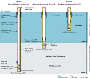
5 Figure 2.1: Required bore properties for aquifers at different depths. (Cockatoo Coal 2013)
2.2.2 Bore water pollution and contaminants
6 2.2.3 Toowoomba Regional Bores
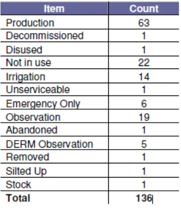
[image:23.595.211.389.299.504.2]Up until the latest GIS data review of Toowoomba’s bores it was believed that the Toowoomba region was home to over 300 bores (Toowoomba Regional Council 2012). ‘Upon closer examination and field inspection, a number of the listed items were incorrectly shown. A detailed review was then conducted over a period of several months to update the bores register with missing, wrongly located and items that were not bores. The reduced total is 136 bores without including any monitoring bores at waste disposal centres or treatment plants’ (Toowoomba Regional Council 2012).
Table 2.1: Bore type counts for various uses (Toowoomba Regional Council 2012).
2.2.4 Characteristics of pumps
7 2.2.4.1 Centrifugal Pumps
The centrifugal pump is a pump that relies on an impeller to move fluid. “The centrifugal pump creates an increase in pressure by transferring mechanical energy from the motor to the fluid through the rotating impeller” (Grundfos 2006). “The centrifugal pump is the most used pump type in the world” (Grundfos 2006). “The principle is simple, well-described and thoroughly tested, and the pump is robust, effective and relatively inexpensive to produce” (Grundfos 2006). For this project it is mainly the impeller sizing, pump curves and pump efficiency characteristics that are of concern.
2.1.4.2 Turbine pumps
A turbine pump is essentially a vertically mounted centrifugal pump (Pump Scout 2014). The turbine pump is most commonly used to draw fluid from deep wells (Pump Scout 2014). For deeper wells, multistage systems are used. Therefore, since bore pumps are typically located up to hundreds of metres underground, the pump will have multiple stages. These stages are mathematically dealt with by multiplying the flow by the number of stages (Grundfos 2006).. A single stage pump implies that there is only one impeller i.e. an X stage pump will have X impellers (Grundfos 2006).
2.2.4.3 Impeller size
8 2013). It is now good practice to select a pump with an impeller that can be increased in size permitting a future increase in head and capacity (Satterfield 2013).
2.2.4.4 Pump Efficiency
“The overall efficiency of a centrifugal pump is the product of three individual efficiencies—mechanical, volumetric and hydraulic” (Evans 2012). “Although mechanical and volumetric losses are important components, hydraulic efficiency is the largest factor” (Evans 2012). The overall efficiency of a pump can be calculated by the ratio of the water output power to the shaft input power and is illustrated by the equation (Evans 2012):
Equation 1
where:
Ef = Efficiency
Pw = the water power
Ps = the shaft power
If the water power equals the shaft power the pump would be 100% efficient. This is never the case though since there will always be losses present (Evans 2012). It is common for smaller pumps to fit within the 50-70% efficiency bracket and larger pumps to fit within the 75-93% bracket (Evans 2012).
9 can improve its efficiency and thereby reduce pumping costs” (Richards & Smith 2003).
2.2.4.5 Pump Performance Curves
10 Figure 2.2: Simple pump curve for system of 30(m^3/hr) flow and 50(m) head (Pump-Flo 2014).
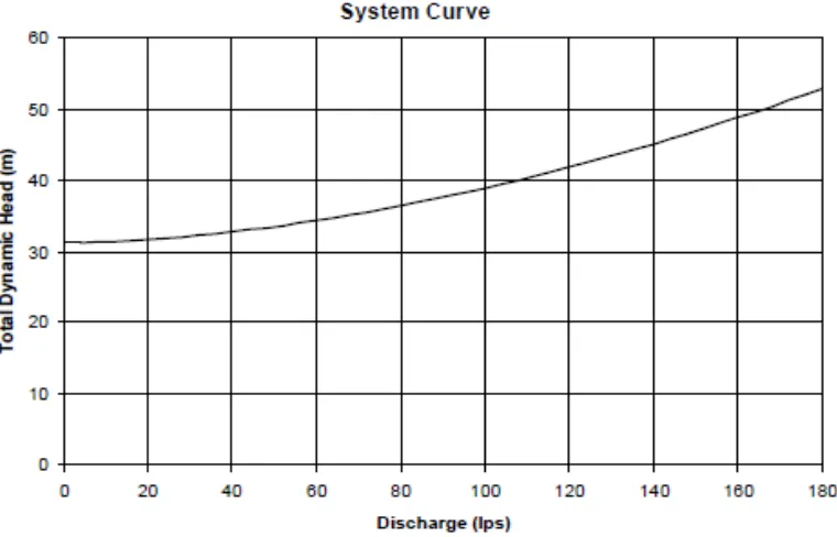
11 Figure 2.3: Simple system curve. (Richards & Smith 2003)
12 Figure 2.4: Operating Point (Spirax-Sarco 2014).
2.3 Modeling
Software
To effectively model Cambooya’s municipal water network, hydraulic modeling and simulation software must be investigated. As there is a large range of varied hydraulic modelers to choose from, software from both internet and database browsing efforts will be briefly analysed. This analysis will include anecdotal evidence from online reviews as well as first hand testing. The first hand testing, however, will only be performed on available freeware rather than introducing a financial requirement for products that may not be ideal for the task. If by the online reviews and advertised abilities a program with financial requirement is selected as the preferred software it will be noted in the dissertation but the most preferred freeware will be used instead so as to avoid any extra cost.
13 EPANET (Free by EPA)
InforWater (By Innovyze)
HydrauliCAD (By HydrauliCAD Software) WaterGEMS (By Bentley)
WATSYS, also known as WaterMax (By HCP) WATHAM (Free by HCP)
Database browsing resulted in much fewer results although these programs were discussed in great depth. This type of search was very effective because the results were more valuable than that of the internet browsing results. The insight into each program at a scholarly level was more helpful than online reviews from people without any qualifications and sale pitches from software developers. The database browsing results include:
WaterCAD (By Bentley Systems) EPANET (By EPA)
From both of these searches combined there were a total of eight results with seven of these being unique. The only overlapping program was EPANET.
From the seven different software options available from these searches there was a great variance in capability, usability and cost. The most relevant of these attributes is capability. The program must be capable of performing the task of modelling and running simulations for a section of the Cambooya’s municipal water supply. These mandatory capabilities include:
The program should be able to emulate pipes, nodes (pipe junctions), pumps, valves and storage tanks or reservoirs.
The program will be able to track the flow of water in each pipe, the pressure at each node and the height of water in each tank throughout the network during a simulation period comprised of multiple time steps. The program will be able to present results in both tabular and graphical
14 The program will be able to upload map files so that the model can be drawn to scale. If these map files also included a three dimensional aspect, so as to include altitudes at any location, this would also be ideal.
The second most important attribute for these programs to have is usability. Usability will directly affect how long it takes to complete the construction and simulation processes. The simpler and more user friendly programs will be chosen over the difficult (but possibly more accurate) software due to the constraint of time. Therefore the requirements for usability include:
The software must be user friendly and very easy to learn. If online tutorial videos are available online that software would become very appealing.
The program should permit simple modification and editing throughout the construction and simulation procedures.
The final requirement that the software must meet is financial. EPANET and WATHAM were the only freeware options, whilst the others had a financial factor ranging between $50 and $300 AUD. So these were the only two programs that would be considered for the modeler of this project.
2.3.2 Further discussion on database browsing results
2.3.2.1 WaterCAD (Bentley systems)
15 2.3.2.2 EPANET
This software was used in the scholarly article discussed later in section 3.3.2.3. In this article the authors were modeling the municipal water supply in Beijing city, China. The model images were very detailed and gave a good understanding of what EPANET offers. They use EPANET in parallel with a GIS .map file. This file contains all the geographical and topographical information of the desired area, making model design a much simpler task. In this report the authors also introduce water reclaiming stations which are essentially recycling stations. After water is processed through this plant it is discharged back into the system. The principle of scattered water induction into a municipal water supply is shared in this project, making EPANET a very appealing software choice.
2.4 Documentation and reports
2.4.1 Toowoomba Regional Council - Bore monitoring bore review
The bore monitoring reports for the year 2012 has been made available by the Toowoomba Region council. This annual report is based on a July – June period similar to the financial year. The report is in a report document goes into depth on the groundwater status of different aquifers around the Toowoomba Region and how they have been performing since the drought. It discusses what observation bores the Toowoomba Regional Council has and how monitoring can be improved with the existing infrastructure. The document includes:
Rainfall and rain gauge data from the period, July 2011 to June 2012 GIS data review
Monitoring system review Monitoring bore records Appendices
16 and averages in millimeters. Whilst rainfall data is not imperative to this project, the data will give a greater understanding of the groundwater behaviour in respective areas.
The ‘GIS Data Review’ includes an overview of the current quantity of bores and their different roles. The document explains how this has changed over the past 12 months as there were many items that were incorrectly shown. That is, items marked as bores were missing, wrongly located or not actually bores. The GIS review itself is not required for this project but the act of the review reinforces the credibility of the data used throughout the modeling process.
As the bore population changed in that 12 month period a bore monitoring system review had to occur. In this review the Toowoomba regional council reevaluated how they were using all the bores. While the role of some bores stayed the same other bores’ role changed depending on their location and aquifer type. The majority of the changes were bores that were swapped from a ‘Not in use’ status to an ‘Observation’ status and vice versa. Approximately 70% of these changes were made within the Toowoomba city. The other 30% were external to the city but within the Toowoomba region.
The millennium drought had a devastating effect upon the bores in the Toowoomba region (Toowoomba Regional Council 2012). Although there has been ground water recharge since the end of the drought, some aquifers are still yet to reach their pre drought condition. To monitor this, the Toowoomba Regional Council records the groundwater changes within the Toowoomba city. The standing water levels of Toowoomba’s bores are recorded monthly into a database so that the average annual level can be calculated. This data will be imperative when including groundwater levels into the model as it will have a notable effect on the acting pump system and ultimately the discharge of the bore into the municipal water supply.
Appendices included:
A map of the current Toowoomba region’s rain gauge stations. A map of the average annual rainfall.
17 Toowoomba’s regional bore data.
A multitude of maps depicting bore locations around the Toowoomba region.
Monthly and annual graphs for each rainfall recording station around the Toowoomba region.
Of these appendices only the regional bore data and bore maps will be relevant to the modeling process. The rainfall data will be relevant to groundwater discussions but will not directly affect the results of this project.
2.4.2 Toowoomba Regional Council - Groundwater bore register – Water and Waste
Strategy and Coordination (WWSC)
The groundwater bore register for 2013 has been made available by the Toowoomba regional council. This document contains information regarding the region’s bores, groundwater aquifers, groundwater vulnerabilities and general land use.
2.4.2.1 Mapping
The document includes maps of bore locations, groundwater aquifers, groundwater vulnerabilities and general land use. These maps are available for the regions:
Toowoomba Region
Millmerran/Brookstead/Pittsworth
Wyreema/Cambooya/Greenmount/Nobby/Clifton Kulpi/Haden/Goombungee/Oakey/Kingsthorpe Highfields
Toowoomba City Cecil Plains.
18 2.4.2.2 Bore register
The bore register has all the information for each individual bore in the Toowoomba region. It includes valuable information such as
Bore and Scheme name – When discussing the bore pumps with
Toowoomba regional council representatives it will be helpful for them and myself if they knew exactly what bore/s were being discussed. This information does not have any great relevance to the topic or model. Location – The specific location of each bore will be helpful in the same
way the ‘Bore and Scheme name’ is, but it will also assist when transferring and comparing the bore register details to the TRC online mapping application.
Purpose – Each bore has a specific purpose such as ‘Town Water Supply’, ‘Irrigation’ or ‘Amenities’, this information is imperative in determining which bores can be used for the model and which cannot. The only bores that will be relevant in a modeling situation is those which have the sole purpose of ‘Town Water Supply.’ There would be no point in modeling any other bores for this project topic.
Status – Bore status is also crucial in bore selection. If a bore’s status is ‘Decommissioned’, ‘Not in use’, ‘Emergency only’, ‘construction’ or ‘Irrigation’ it will be of no use to this project. The only bores that will be shortlisted in selection will have a ‘Production’ status.
Original drill date and expiry date – The age of the bore is also of large
concern in this topic. If a bore has a relatively recent drilling date one would assume that the bore is entirely intact and running efficiently. Bores that are closer to expiry date, however, could have some faults present. These faults include, damaged filters, high chemical levels (i.e. nitrate) or damaged pipe casing. Apart from damaged or blocked filters, these faults should not have any effect on the physical testing results. The age of a bore will not be a determining factor in bore selection but if the results skew then the age of the bore may come into mention.
19 Certain aquifers may behave differently to others and this will be noted in the discussion of results.
2.4.2.3 Bore log data
The bore log data sheets contain very similar information to the bore register but also include helpful additional data such as:
Bore Depth (m) – The bore depth will be required when discussing
groundwater levels and pump requirements.
Flow rate (L/s) – The flow rate of the bore is required for determining the
speed at which the pump is running and/or the impeller size.
Coal seam gas / Petroleum impacts – Whilst this information is not relevant to the model or physical testing, it is still an issue of sustainability around this project topic.
Also attached to this document is a report on ‘Groundwater vulnerability and availability - Mapping of the upper condamine river catchment.’ The report is a Masters level dissertation by Allen Hansen from the University of Technology, Sydney. The dissertation focuses on climate, geology, surface water hydrology, groundwater mapping techniques and groundwater availability. Whilst, most of this report has no relevance to the topic of this project, the data gathered for the groundwater mapping techniques and the groundwater availability sections are very informative towards groundwater discussions. Information such as groundwater depths and net recharge rates are extremely relevant to this topic.
2.4.3 Evolving effective hydraulic model for municipal water supply – Wu, Zheng Y
(Bentley systems)
20 Data requirement
Calibration framework Implementation
Data collection
Calibration target, boundary and demand data Flow balance calibration
Hydraulic grade calibration Model application
The article also discusses the use of a hydrant tagging system and Competent Darwinian Evolver software which further assists decision making.
Whilst the goal of this project is not to create a hydraulic modeler from scratch like this article describes, it gives a better understanding of what is required in creating the software that will be used and the data that will be needed before the model can be created.
2.4.4 Pipeline network modeling and simulation for intelligent monitoring and
control
21 34 links vs the 14 nodes and 14 links model in the FORTRAN system, it does not differ significantly. Therefore the former model is used as the working model. This generates results on the dynamic change of water level in the reservoirs, which are then used as input in the expert system developed for the monitoring and control of the water supply system.’(Kritpiphat, Tontiwachwuthikul & Chan 1998) Because the software the authors chose for this analysis were programming based modellers they will not be used or discussed any further in this paper.
This paper is similar to that discussed in 3.3.3 but goes into a much greater depth mathematically. This article shows both the implemented arithmetic and discusses the different hydraulic methods that can be used rather than just being specific to the one method.
2.4.5 Hydraulic model for multi-sources reclaimed water pipe network based on
EPANET and its applications in Beijing, China.
22
3. METHODOLOGY
3.1 Introduction
In this paper, a method is proposed to increase the understanding of the relationship between a small water network’s supply pressures and local contributing bores. This was possible by creating a hydraulic model of a water supply network within the Toowoomba Region and calculating the pressures at different demand periods and comparing that to results that were physically collected from the region. To accurately perform this analysis a lot of data was required.
3.2 Choosing the software
23 After these required specifications were identified the search was narrowed down to an internet based search and a database search. As expected the internet results gave many more responses than the database results. From the internet based search there were six programs nominated for further discussion, two of these were freeware and downloadable online. In the database search there were two programs chosen, both of which were freeware and downloadable online. There was one simulator which overlapped out of the four freeware results and that was EPANET. This software was simple, free and included GIS integration which would allow the upload of ‘.map’ files. Therefore EPANET was the chosen software for this project.
3.3 Data Requirements
In the literature discussed in section 2.3.5, it mentions the use of EPANET and the data requirement plan for a project that would be very similar to this one. Below is a network flow diagram of what data would be required and what processing the gathered data would follow in order to give an output (Kritpiphat 1998). It has been determined that this would be a fitting model for the creation of this project.
24 The data input would include:
Pipe discharge. Pipe diameters.
Pipe friction factor and/or minor loss coefficients.
Water pressure at specific points (this may be calculable via the geographical data plus the present time pressure head at the gravity feeding reservoirs).
Pump size. Pump Curve.
Elevation data across the entire modeled section. Total head at reservoirs.
Stagnant head of bores. Acting pump pressure.
All the information on pipes would be gathered from Toowoomba Regional Council’s online mapping application. All pipe diameters, discharges, materials, install dates and operational statuses could be determined using the ‘Identify’ tool within the online application. Information on the pumps, however, is much more difficult to attain. The council does not yet have a bore pump register although they have just recently started collating data for such a document. This information would therefore be attained via Toowoomba Regional Council employees. Before this information can be gathered, however, a location must be selected.
3.4 Location
3.4.1 Location Requirements
25 and the source as this would further complicate the analysis. It is preferred that these bores also be outside of the CBD so that discharges and water requirements are consistent and reasonably similar across the field of analysis. If the location was within the CBD, water requirements would vary greatly during the period of data collection. This is because of the variance in business types using different amounts of water depending on the time of day and the number of customers/workers present during the period of data collection. Therefore, a small amount of data from CBD areas would not necessarily accurately reflect the pressure distribution.
In residential areas water usage will be much more uniform across the area of analysis and peak times are very likely to be consistent during the week. Therefore residential areas are the preferred location of analysis. It would also be ideal if there was only one service main feeding into the area of analysis from one reservoir, this would make the analysis much simpler as water would only be feeding into the system from a single direction. If this is not possible or an area like this cannot be found then a location with the greatest possible isolation will be used.
3.4.2 Selected Location
26 3.4.2.1 Location population data
There has been no population evaluation in Cambooya since 2012 therefore the councils’ predictions and estimations will be used to determine a current population. The population of Cambooya has been estimated using the Council’s equivalent persons (EP) estimations between 2012 and 2031 in 5 year intervals. These estimations were interpolated to derive a population for the year 2014. There is also an ultimate EP which represents the EP value when Cambooya is at a point of maximum development. The EP values from 2012-ultimate are illustrated in the table below.
Table 3.1: Equivalent Persons spanning from 2012 - ultimate development. (Toowoomba Regional
Council 2012)
Using this data, the current population was determined to be approximately 1340 EP. This was found by interpolating between the ‘existing’ and 2016 EP predictions.
3.4.2.2 Cambooya Overview/Layout
27 Figure 3.2: Overview of the chosen location of analysis.
3.4.2.3 Number of residential properties (layout of area with imagery)
28 will be divided among the residential lots so that an average demand per residence can be determined.
The number of residential properties was counted using the TRC mapping application. The application gives the option to show a satellite image as the background of the map. Whilst the counted number will not likely be 100% perfect due to non-residential properties or abandoned lots, it will give a reasonable number to assume as an average for the model. To most accurately count the populated allotments the driveways were considered while counting to safeguard against counting large sheds or detached garages. The following image illustrates the Cambooya overview with satellite imagery included.
29 Whilst it would be near impossible to count the populated allotments from this image, the application incorporates an excellent ‘zoom in’ function. An example of this zoom (at only 90%) is shown below in figure 4.8.
Figure 3.4: Satellite image of property (90% zoom)
30 3.4.2.4 Diurnal pressures and demands
The existing unit demand has been calculated based on the council’s historical data for water consumption across all properties connected to the Cambooya water supply network. ‘The unit demand for all future planning horizons was obtained from the ‘Determination of Flows for Planning Purposes across the Toowoomba Region’ report (TRC 2011) and the ‘Draft Water Infrastructure Policy no. 2.3’
(TRC 2012)’(Toowoomba Regional Council 2012). ‘Non-revenue water was calculated based on the actual bore production and water consumption data’ (Toowoomba Regional Council 2012). Non-revenue water is applied as a constant demand (Toowoomba Regional Council). Cambooya’s residential and non-residential peaking patterns and corresponding demands are shown in the images below.
Figure 3.5: Average Cambooya water consumption – Peaking Factor vs. Time. (Toowoomba
31
Demand data 2012 2014 Ultimate
Total population 1288 1340 2641
No. of Houses ? 391 ?
People per house (AVG) 3.43 3.43 3.430
L/EP/d 147.3 150 200
L/EP/s 0.00170 0.00174 0.00231
L/s/household 0.00585 0.00595 0.00794
Non-revenue (L/s) (12.8%) 0.28 0.29778 0.50895
AD (L/s) 2.2 2.629 4.500
MDMM (L/s) 3.71 3.932 10.330
PD (L/s) 5.34 5.653 14.860
PH (L/s) 11.46 12.144 31.910
Table 3.2: Demand predictions from 2012 –ultimate development. (Toowoomba Regional Council
2012) - AD = AVG Day, MDMM = Maximum Day Mean Month, PD = Peak Day, PH = Peak
Hour.
From these figures and an excel spreadsheet that replicates the process that the TRC used, the demand values for 2014 have been determined. The following table shows all 2014 demand figures that will be used in the EPANET model.
32 3.4.2.5 Cambooya Reservoirs
There are currently two reservoirs in Cambooya, one newly constructed and one recently retired. The two reservoirs have the following properties.
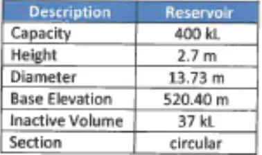
[image:49.595.185.374.186.298.2]Table 3.4: Retired reservoir properties (Toowoomba Regional Council 2012).
Table 3.5: New reservoir properties (Toowoomba Regional Council 2012).
33 Figure 3.6: Cambooya’s recently retired 400kL reservoir.
34 Figure 3.8: Cambooya’s new 1.5ML reservoir 2/2.
3.4.2.6 John Street Bore
The John Street bore is the lead bore for the township’s supply (Toowoomba Regional Council 2012). As per tender information the duty point is 15L/s at 144m head and the pump is at a depth of 100m. All elevation data for John Street bore is shown in table 4.7.
Table 3.6: John St bore elevation data (Toowoomba Regional Council 2012).
35 Figure 3.9: John St bore electric motor drive.
36 Figure 3.11: John St bore chlorination control unit.
37 3.4.2.7 George Street Bore
The George Street bore is the auxiliary supply for Cambooya (Toowoomba Regional Council 2012). When operating, the George St bore creates a ‘milky’ colour in the reticulating water (Toowoomba Regional Council 2012). In order to avoid this, the council always has the John St bore activated after the George Street bore has turned off (Toowoomba Regional Council 2012). This flushes the unwanted ‘milky’ colour out of the reticulation (Toowoomba Regional Council 2012).
“The duty point of the George Street bore is 20L/s and 149m head” (Toowoomba Regional Council 2012). The pump is installed at a depth of 100m, the same depth as John Street (Toowoomba Regional Council 2012). All other elevation data is shown below in table 3.7.
Table 3.7: George St bore elevation data (Toowoomba Regional Council 2012).
38 Figure 3.13: George St bore flow rate.
39 Figure 3.15: George St bore chlorination concentration.
3.4.2.8 Pump properties
40 Figure 3.16: John Street bore pump label.
Figure 3.17: George Street bore pump label.
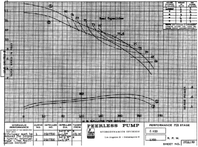
41 The following images are of the 150 RM pump curve, the TRC’s partial 6HXB curve and a larger 6HXB curve from the Peerless Pumps website.
Figure 3.18: 14 Stage 150 RM Pump curve (John Street pump)
42 Head (m) Flow (L/s)
230 0
225 2
200 12
165 17.5 150 20.5
137.5 22
122 23.5 100 25.5
50 27
0 28
[image:59.595.84.490.86.388.2]20 Stage 6HXB
Figure 3.20: Peerless Pump’s Imperial pump curve for 20 stage 6HXB (George St Pump).
From these curves the following pump data was derived. Where flow or head measurements were not given values they were approximately but carefully interpolated.
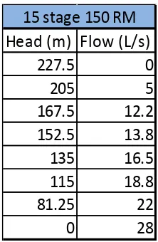
[image:59.595.240.346.533.727.2]43 Head (m) Flow (L/s)
227.5 0
205 5
167.5 12.2 152.5 13.8
135 16.5
115 18.8
81.25 22
0 28
[image:60.595.261.372.83.253.2]15 stage 150 RM
Table 3.9: 15 stage 150 RM pump curve in tabular form.
These values will be used in the EPANET model as the input data for the respective pump curves.
3.4.2.9 Pipe properties
The vast majority of pipes in the selected location are PVC-U pipes, however, there are a few iron ductile, PE100 and Blue Brute pipes scattered throughout (Toowoomba Regional Council 2014). The PE100 and Blue Brute materials have extremely similar roughness values as the PVC-U (Duronil 2007) and are therefore given the same roughness of 0.0015mm. The Iron ductile pipes have a much greater roughness value of 0.03 (Duronil 2007). Any pipes that have an unknown material will be assumed to be PVC-U pipes.
The pipe diameters vary greatly throughout the system. The 100mm and 150mm pipes are the most common sizes, but 80mm pipes and 200mm pipes are also used at low and high flow points respectively. The two pipes that attach the bores to the rest of the network have a diameter of 600mm; these pipes are considered to be detention basins for the chlorine to mix in with the water before entering the reticulation (Toowoomba Regional Council 2012).
44 3.3.2.10 Cambooya’s groundwater source
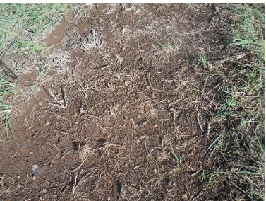
[image:61.595.108.485.254.538.2]Cambooya’s bores are extracting from an aquifer type known as ‘Main Range Volcanics’ (Hansen, A 1999). The Main Range Volcanics consist predominantly of tertiary basalts with various trachyte flows, breccias and truffs (Hansen, A 1999). The soil cover is dominantly black cracking clay type soils with lesser red non-cracking clay soils (Hansen, A 1999). This type of soil is present throughout Cambooya, as shown in the figure 3.21.
Figure 3.21: Cambooya soil.
The groundwater found in this type of aquifer is typically potable and yields can range from almost nothing up to 80L/s in isolated areas (Hansen, A 1999). This level of discharge occurs at the bore south of Jondaryan (Hansen, A 1999).
45
3.4.2.10.1 Recent groundwater behaviour
46 Value John St George St Percentage Local minimum 121.00 133.00 45.96%
AVG 121.86 133.71 47.25%
Local maximum 122.00 134.00 47.93%
Difference (m) 1.00 1.00 N/A
Difference (%) 0.9918% 0.9925% 1.97%
Minimum 98 110 1%
Maximum 149 161 100
Derived values Data based on period 23/06/14 - 04/08/14
Minimum and Maximum groundwater levels for Cambooya
bores
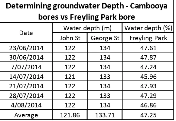
Water depth (%) John St George St Freyling Park
23/06/2014 122 134 47.61
30/06/2014 122 134 47.87
7/07/2014 122 134 47.24
14/07/2014 121 133 45.96
21/07/2014 122 134 47.93
28/07/2014 122 133 47.29
4/08/2014 122 134 46.86
Average 121.86 133.71 47.25
Date Water depth (m)
Determining groundwater Depth - Cambooya
bores vs Freyling Park bore
Table 3.10: Data to determine maximum and minimum water depths for Cambooya bores.
[image:63.595.109.400.86.286.2]From this data the minimum and maximum groundwater levels for John and George St have been determined. These values are illustrated in table 3.11.
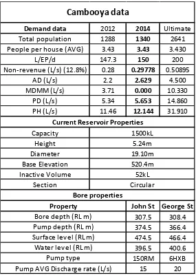
47 Demand data 2012 2014 Ultimate
Total population 1288 1340 2641
People per house (AVG) 3.43 3.43 3.430
L/EP/d 147.3 150 200
Non-revenue (L/s) (12.8%) 0.28 0.29778 0.50895
AD (L/s) 2.2 2.629 4.500
MDMM (L/s) 3.71 0.000 10.330
PD (L/s) 5.34 5.653 14.860
PH (L/s) 11.46 12.144 31.910
Capacity Height Diameter Base Elevation Inactive Volume Section
John St George St 307.5 308.4 374.5 366.4 474.5 466.4 396.5 400.6 150RM 6HXB 15 20
Current Reservoir Properties 1500kL
5.24m 19.10m
Pump AVG Discharge rate (L/s)
Cambooya data
52kL Circular Bore properties
Pump type Surface level (RL m)
Pump depth (RL m) Bore depth (RL m)
Property
520.4m
Water level (RL m)
This data is only viable due to the assumption that groundwater levels across the aquifer share a uniform depth percentage. In reality, this would not be the case and the extreme groundwater depths would most likely differ. However, the input of these depths into the model will still give a great representation of how Cambooya’s water supply pressure varies with these extreme depths.
3.4.2.11 Cambooya data collated/tabulated.
[image:64.595.130.415.313.714.2]The data that will be used in the construction of the EPANET model is included in table 4.11.
48
3.5 Modeling
3.5.1 Model Planning
Using the aforementioned data, the model will be constructed using EPANET, ideally with an uploaded ‘.map’ file of the area in question. The model will include the construction of virtual pipes, nodes, pumps, reservoirs, tanks, junctions and valves that imitate a location within Cambooya’s network. This will all be to topographical and geographical scale. If the ‘.map’ file can’t be attained an image of the overview of the location of analysis will be pinned to the EPANET background. The image will be made to scale and the pipeline will be drawn directly over the top of it. The altitude of each important node on the map will then be gathered and manually added to the model.
3.5.2 Model Construction
As this program had not been used before online tutorials were completed. These online tutorials gave step by step instructions of how to setup, create and run a model. Unfortunately these tutorials only included the construction of smaller, simple water networks so there was still an extensive debugging period before the model would run.
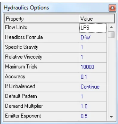
3.5.2.1 Hydraulic Options
49 Figure 3.22: Chosen hydraulic properties for the EPANET model.
3.5.2.2 Background image scaling
The next step was to seek out a .map for the Cambooya region. As explained in 4.4.1 attaining a .map file of the Cambooya area would be extremely advantageous and significantly reduce the data input period by eliminating the requirement of inputting node elevations. This map would have also included a layout of the Cambooya pipe network so that nodes and pipes could be correctly placed. Unfortunately, however, it was not possible to attain this file.
50 Figure 3.23: Screenshot taken from TRC online mapping application for use in scaling EPANET
model.
Note the clarity of the scale and water network layout (blue lines).
51 field. After multiplying the maximum dimension lengths by this ratio, the map would then be to scale.
3.5.2.3 Adding physical components
The next step was to place nodes at the ends of where pipes will be placed and areas of interest. The areas of interest were the positions of homes where physical data was collected from. After placing all nodes in their desired locations the pipes would be added. These pipes are simply drawn between nodes while the auto-length option is set to be ‘on’. This ensures that all pipes that are drawn will be matched to the set scale size. Completing this task manually would have extended the model construction period significantly.
Since the general layout of the network had been set, it was time to add the reservoirs, tanks and pumps. A reservoir in EPANET is defined as an ‘infinite source of water’ (Rossman 2000). Since the volume of groundwater in the area is so substantial in comparison to the amount of water that is used, the two bores were set as reservoir nodes. Therefore, the Cambooya reservoir was not technically a reservoir in EPANET and had to be set as a tank node. A tank is ‘a container of water whose dimensions can be defined’ (Rossman 2000). The Cambooya tank is situated above the township and therefore does not require a pump therefore a pump has not been allocated to it in the model. The two bores, however, are both introduced into the network via their respective bore pumps and will therefore require pumps in this model also.
3.5.2.4 Component properties
Since the physical components of the network had been setup the next step was to input each component’s specific properties and attributes.
3.5.2.4.1 Node properties
52 Figure 3.24: Node (junction) 7 properties.
53 Figure 3.25: Cambooya overview showing nodes with positive demands.
54
Demand Position No of houses Demand (L/s)
1 0 0
2 5 0.029971228 3 13 0.077925192 4 4 0.023976982 5 1 0.005994246 6 14 0.083919437 7 8 0.047953964 8 7 0.041959719 9 12 0.071930946 10 3 0.017982737 11 8 0.047953964 12 12 0.071930946 13 6 0.035965473 14 20 0.11988491 15 13 0.077925192 16 9 0.05394821 17 6 0.035965473 18 5 0.029971228 19 5 0.029971228 20 7 0.041959719 21 9 0.05394821 22 4 0.023976982 23 18 0.107896419 24 3 0.017982737 25 9 0.05394821 26 16 0.095907928 27 24 0.143861893 Total right 241 1.444613171 X 40 0.239769821 Y 40 0.239769821 Z 70 0.419597187 Total left 150 0.899136829 391 2.34375 12.8% Non-revenue - 0.3
Absolute total 391 2.64375
[image:71.595.210.406.298.725.2]portion of Cambooya that has not been included in this model. Since, in reality, this system will also be supplying to that side of Cambooya, their water requirement could not be ignored. Nodes 2-27 each represent a portion of houses in the modeled section of Cambooya. The number of houses with corresponding demand values has been collated into table 3.13. Node 1 is not present in figure 3.25 as it was used as an example in table 3.13, showing that when there are no houses in the area the demand is equal to 0. Also included in table 3.13 is the non-revenue water requirement, which, as per the Toowoomba Regional Council, is equal to 12.8% of the AD flow
55
Demand data 2012 2014 Ultimate
Total population 1288 1350 2641
No. of Houses ? 391 ?
People per house (AVG) 3.45 3.45 3.453
L/EP/d 147.3 150 200
L/EP/s 0.00170 0.00174 0.00231
L/s/household 0.00589 0.00595 0.00794
Non-revenue (L/s) (12.8%) 0.28 0.30000 0.50895
AD (L/s) 2.2 2.629 4.500
MDMM (L/s) 3.71 4.261 10.330
PD (L/s) 5.34 5.653 14.860
PH (L/s) 11.46 12.144 31.910
The demand values for these nodes were estimate using table 3.14. This table assumes that there is currently a population of 1350 in Cambooya this year and that each house has an average of 3.45 people. The values for the AD, MDMM, PD, PH, the Non-revenue flow requirement and the water volume per person per day were all extrapolated from the Cambooya Water Supply Scheme of 2012.
Table 3.14: Calculator for Cambooya demand averages.
3.5.2.4.2 Pipe properties
56 Figure 3.26: Pipe 1 properties.
The pipe material can be found using the identify tool on the TRC’s online mapping application. With this pipe material, a corresponding roughness value can be found. As 95% of the pipe material in Cambooya is PVC-U the roughness was typically 0.0015mm as shown in figure 3.26 for pipe 1.
The online mapping application could also define the pipe diameters throughout the network. As shown in figure 3.26 the diameter was found to be 200mm.
Pipe length was typically not an inputted value as the scaling and auto-length function of EPANET automatically determined the lengths of each pipe. For pipe 1, however, the length was manually inputted because it is the pipe which connects the reservoir to the network. If to scale, this pipe would be a considerable distance off the page and would therefore be harder to display. To manually input this value, auto-length had to be set to ‘off’. This made the length input area available to customisation.
57 3.5.2.4.3 Reservoir properties
The next properties added to the model were that of the reservoirs. These reservoirs were to emulate the George and John Street bore as closely as possible. The only property required for the reservoir is the Total Head. This value is equal to the depth of the pump plus the water level above the pump. In this instance it was 366.4m RL (Pump depth) + 34m (Water above pump). Figure 3.27 illustrates the reservoir properties of, Reservoir R2
Figure 3.27: Reservoir R2 properties.
3.5.2.4.4 Tank properties
58 This will be one of the key modifications in configuring the overall model to match the physical data. The minimum level section represents the minimum level that the reservoir can reach without shutting down. Again, this is mostly required for the ‘over time’ simulations but is still a required property for the model to run. The maximum level represents the height of the tank. Since the Cambooya Tank (Reservoir) is 5.24m high, the value can also be adopted for the model’s tank maximum level. The diameter of the tank is shown to be 19.2m in section 3.3.2.5 of this document. Therefore this value will be adopted for the model’s tank diameter also. Figure 3.28 illustrates the values for Tank T1.
Figure 3.28: Tank T1 Properties
3.5.2.4.5 Pump properties
59 Figure 3.29: Pump P4 properties
As shown in figure 3.29, a pump curve named ‘JohnSt’ has been added into this field. This curve was created in the Edit_Curve section of EPANET. Figure 35 shows the JohnSt curve which emulates the values found in table 10 of section 3.3.2.8.
[image:76.595.125.478.471.741.2]60 The table on the left side of figure 3.30 is where the values for flow and head are added. The curve on the right is automatically drawn after the values are entered.
3.6 Assumptions
For EPANET to run models without excessive complications, assumptions had to be made within the software. The assumptions that EPANET make include: All pipes are full at all times (Rossman 2000).
The pump supplies the same amount of energy, no matter what the flow is unless a pump curve is supplied (Rossman 2000).
Water within tanks is assumed to be completely mixed (Rossman 2000). Any component properties that are not given a value are assumed to be 0 or
the default (Rossman 2000).
The Darcy Weisbach Equation, which has been chosen within EPANET as the preferred method for dealing with pipe friction loss, also makes some assumptions. The assumptions that this equation makes include:
For liquid flow, the density of the fluid flowing in the system is constant (ABZ 2010).
Like EPANET, Darcy’s equation assumes full pipe flow (ABZ 2010).
For this specific model to run, more assumptions still had to be made. These assumptions are not related to the software used but the scenario that is being modeled. These assumptions include.
Neglecting non-residential water demands (i.e. school, bowls club and pub). This is because the water usage data for these locations was unavailable.
61
3.7 Model Debugging
Initially, after the components of the model were all added and the specific data for each component inputted, the model would not run. There were massive negative pressures throughout the network, suggesting that the demand was not being met through the entire system. Whilst this was the only issue that the model had it was one that was not easily found and solved. Initially, it was thought that the pump data had not been entered correctly since the curve did not initially extended to 0 head and 0 flow. This was then fixed but the model would still not run. After going through the EPANET manual it was eventually discovered that the pipe size had to be entered in in millimeters. This was despite the fact that at the commencement of the project the units were set to metres. This was apparently just a selection between imperial and metric units.
3.8 Field work
3.8.1 Toowoomba Regional Council water supply system tour.
After approaching the Toowoomba Regional Council about all the required data for this thesis, a southern district Water & Sewage Operations Coordinator, Damian Darr, offered a tour of the Cambooya water infrastructure. This tour included visits to the George Street and John Street bore pump houses as well as the old and new Cambooya reservoirs. The infrastructure seen during this tour is included in section 3.3.2.5 to section 3.3.2.8.
62 Figure 3.31: George St bore chlorination control unit & Sodium Hypochlorite basin.
63 Figure 3.32: Acute & Chronic health effects of Sodium Hypochlorite.
Figure 3.33: Sodium Hypochlorite First aid and handling instructions
3.8.2 Data collection plan
[image:80.595.126.467.362.621.2]64 taps of 20-40 Cambooya homes at high and low demand times during the day. These readings will then be collated and used as a guide for model configuration. The results will also be graphed against the model results so that comparisons can be made. From these comparisons recommendations will be given and the effect of any assumptions will be discussed.
3.8.3 Data collection activities
All of the physical data required for this project was attained over three visits to Cambooya. Two of these activities were performed from approximately 10am-1pm during the week for the off peak /low demand period. The other visit was conducted from 6am-830am on a Saturday morning which was assumed to be a higher demand period for this location.
3.8.3.1 Off-Peak/Midday collection
Whilst conducting these activities it was important to where suitable attire. This was important not only for safety reasons but to impose a sense of professionalism to the community whilst walking from house to house. Therefore, long work trousers and a long sleeved button up shirt were worn with a high visibility TRC vest over the top. This vest was made available through Matthew Norman, a control systems engineer from the TRC. Black steel cap boots were also worn. Whilst these were not necessarily required for the task, wearing them would assist in appearing professional to the community. For protection from the sun, a hat and sunglasses were worn.
To perform the full activity, certain pieces of equipment were required. This included:
A pressure gauge that would attach to residential outdoor taps.
A clipboard with paper and pen for recording all the pressure readings with.
65 A Camera for taking pictures of any noteworthy experiences and important
infrastructure throughout the collection activity.
A wrench just in case the pressure gauge gets jammed on the tap (This happened on the first low demand visit and a wrench wasn’t available). Sunscreen to prevent sunburn throughout the day.
Mobile phone in case of any emergency
Wallet for proof ID and incase money was required for any reason throughout the activity.
Attire and equipment were not the only requirements for this data collection activity. A reasonable considerable amount of common sense also had to be applied when making decisions while walking from house to house. The main decisions that were made revolved around house selection. Aggressive dogs were a huge issue for house visits in this area. They were the main factor that controlled the house selection process. Therefore to deem a house suitable for selection the following guidelines for dog safety were created:
If a house