Phage-Host Interaction in Nature
Thesis by
Arbel D. Tadmor
In Partial Fulfillment of the Requirements
for the Degree of
Doctor of Philosophy
California Institute of Technology
Pasadena, California
2011
Acknowledgments
To many people I owe my gratitude for making my stay at Caltech both fascinating as well as
incredibly fun. First and foremost I would like to thank my advisor, Prof. Rob Phillips, who
taught me how to be the most critical scientist I can be; Prof. Jared Leadbetter, from whom I
learned about microbial diversity and the art of phylogenetics and who graciously agreed to head
my committee, and my two other committee members, Prof. David Baltimore and Prof. Victoria
J. Orphan, for kindly agreeing to be on my committee and whose questions and critique were
critical to the success of my research. I wish to also thank Dr. Eric G. Matson and Dr. Elizabeth
A. Ottesen for kindly answering my many questions, and Eric and Dr. Adam Z. Rosenthal for
going termite collecting with me on several occasions. I would like to also thank Dr. Blake W.
Axelrod, Prof. David Bensimon, Dr. Bertrand Ducos, Prof. Michael L. Roukes and Lijun Xu for
fruitful and fascinating collaborations, and Prof. Grant J. Jensen for allowing me access to his
imaging facility working closely with Dr. Alasdair McDowall and Dr. Bill Tivol. I am also
indebted to the many people who kindly agreed to review our work along the way, including
Prof. Sherwood Casjens, Prof. Daniel S. Fisher, Prof. Roger W. Hendrix, Prof. Ron Milo, Prof.
Stephen R. Quake, Prof. Edward M. Rubin and Prof. Nathan D. Wolfe. I would also like to thank
past and present members of the Phillips group and the Leadbetter group, and especially Dr.
Heun Jin Lee, Dr. Martin Lindén, Damien Soghoian, Dr. David Wu and Dr. David Van Valen for
the many stimulating conversations and valuable feedback I received from them over the years.
Abstract
Table of Contents
Acknowledgments... iii
Abstract ...v
Table of Contents ... vi
List of Figures ...x
List of Tables ... xii
Chapter 1 Introduction
Chapter 2 Probing Individual Environmental Bacteria for Viruses Using
Microfluidic Digital PCR
2.1 Abstract ... 2-1 2.2 Introduction ... 2-2 2.3 Proposed method for phage-host co-localization ... 2-2 2.4 Hunting for phages in the termite hindgut ... 2-3 2.5 Identification of novel uncultured bacterial hosts ... 2-6 2.6 Phage-host cophylogeny ... 2-9 2.7 Conclusions ... 2-12 2.8 References and notes... 2-13 2.9 Appendix ... 2-15 2.9.0 Contents ... 2-15 2.9.1 Materials and Methods ... 2-16 2.9.2 Supporting Text ... 2-34 2.9.3 Supporting Figures ... 2-54 2.9.4 Supporting Tables ... 2-64 2.9.5 References ... 2-80
Chapter 3 MetaCAT—Metagenome Cluster Analysis Tool
Chapter 4 The Biophysics of Prokaryotic and Viral Diversity in Aqueous
Environments
4.1 Abstract ... 4-1 4.2 Introduction ... 4-2 4.3. General assumptions ... 4-4 4.3.1 Decoupling phage-host systems ... 4-4 4.3.2 Host mortality ... 4-5 4.3.3 Virus decay ... 4-8 4.3.4 The physiological state of the host... 4-8 4.3.5 Bacterial and viral abundance distribution ... 4-9 4.4 A biophysical model of phage-host interaction ... 4-9 4.4.1 Model development part I: A single phage-host system ... 4-9 4.4.1.1 Viral diffusion and infection rate ... 4-9 4.4.1.2 Predator-prey relations ... 4-13 4.4.1.3 The virus diffusion constant ... 4-16 4.4.1.4 The virus-to-bacterium ratio for a given phage-host system ... 4-17 4.4.1.5 Correlation between burst size and host/virus dimensions ... 4-18 4.4.1.6 Dependence of host concentration on bacterium size ... 4-21 4.4.1.7 Large bacteria are rare ... 4-23 4.4.1.8 Application of the model to environmental systems ... 4-25 4.4.2 Model development part II: Non-interacting phage-host systems ... 4-27
4.4.2.1 A stochastic interpretation of bacterial and viral parameters ... 4-27 4.4.2.2 A simple evolutionary scenario ... 4-30 4.4.2.3 The size spectra of bacteria in aqueous environments ... 4-31 4.4.2.4 Possible deviation from a uniform distribution ... 4-33 4.4.2.5 Total bacterial concentration ... 4-33 4.4.2.6 Species richness ... 4-34 4.4.2.7 What is a species? ... 4-35 4.4.2.8 Volume of diversity ... 4-37 4.4.2.9 Species density ... 4-38 4.4.2.10 Observed species diversity in nature ... 4-38 4.4.2.11 Bounds on global marine diversity ... 4-40 4.4.2.12 Factors determining species richness ... 4-43 4.4.2.13 The total concentration of viruses and the VBR in the environment ... 4-45 4.4.2.14 Total prokaryotic biomass concentration ... 4-48 4.5 Conclusions and further experiments ... 4-50
Chapter 5 An evolutionary model of phage-host interaction
5.1 Introduction ... 5-1 5.2 Definition of a bacterial and viral strain and species ... 5-3 5.3 A model for bacterial-viral co-speciation ... 5-7 5.3.1 Description of the evolutionary model ... 5-7 5.3.2 A coarse-grained view of the evolutionary model satisfies all the properties of the biophysical model ... 5-13 5.3.3 Revisiting the question of what is a “species”? ... 5-14 5.3.3.1 “Quark-gluon” model of a species ... 5-14 5.3.3.2 The meaning of Nspecies ... 5-16
5.3.3.3 The dynamics of speciation ... 5-21 5.3.3.4 Analogy to the conventional concepts of a “species” and “strain” ... 5-21 5.3.3.5 The insight for the coarse-grained model ... 5-22 5.3 Why do phages typically have a narrow host range? ... 5-23 5.4 Testing the evolutionary model: evolution experiment of a phage-host system ... 5-25 5.5 References ... 5-26
Chapter 6
A Kinetic Model for Stress Fiber Contraction and Relaxation
List of Figures
Figure 1.1 Scaling of the virus concentration, the bacterium concentration and the
VBR with the radius of the bacterium for a single phage-host system 1-8
Figure 1.2 Schematic depiction of bacterial and viral species and strains 1-13
Figure 1.3 Positive feedback evolution model for emerging bacterial and viral species 1-16
Figure 1.4 Total concentration “taken up” by the evolving bacterial strain and its
parental strain 1-17
Figure 1.5 Workflow using the microfluidic digital PCR array for host-virus
co-localization in a novel environmental sample 1-19
Figure 1.6 Ideal clustering of gene objects in a metagenome 1-20
Figure 1.7 End-point fluorescence measured in a panel of a microfluidic digital
PCR array 1-21
Figure 1.8 Map of viral cassettes in ZAS2 and ZAS9 highlighting gene frequency
in the higher termite metagenome 1-22
Figure 1.9 Agarose gel electrophoresis analysis of terminase PCR product
amplified from termite and related insect species 1-23
Figure 1.10 Typical force-time response to Cytochalasin D perturbation 1-25
Figure 1.11 Schematic model for stress fiber relaxation 1-25
Figure 1.12 Stochastic model prediction of force step durations versus experimental
data 1-26
Figure 2.1 End-point fluorescence measured in a panel of a microfluidic digital
PCR array 2-5
Figure 2.2 Phylogenetic relationship between cultured and uncultured bacterial host
rRNA genes and their associated viral DNA packaging genes 2-9
Figure 2.3 Rank abundance curve of free living Treponema spirochetes in R.hesperus
termites identifying putative phage hosts 2-11
Figure 2.4 Workflow using the microfluidic digital PCR array for host-virus
co-localization in a novel environmental sample 2-54
Figure 2.5 Multiple alignment of termite related terminase sequences and closest
homologs 2-55
Figure 2.6 Multiple alignment of pfam03237 with a ZAS-associated terminase 2-57
Figure 2.7 Phylogenetic analysis of retrieved Treponema SSU rRNA sequences and
close relatives 2-59
Figure 2.8 NeighborNet network of termite-related terminase alleles 2-60
Figure 2.9 Example of microfluidic array panel readout after thresholding 2-62
Figure 2.10 Agarose gel electrophoresis analysis of all FAM hits in a microfluidic array
panel 2-62
Figure 2.11 Schematic diagram of a Monte Carlo simulation of microfluidic array
loading and sampling 2-63
Figure 3.1 Ideal clustering of gene objects in a metagenome 3-5
Figure 3.2 An illustration of a BLAST and an iBLAST analysis 3-6
Figure 3.4 Illustration of a final MetaCAT analysis 3-8
Figure 3.5 Example of list of connected KRGs at one of the clustering iterations 3-14
Figure 3.6 MetaCAT main interface 3-15
Figure 4.1 Correlation between burst size and cell volume
with the radius of the bacterium for a single phage-host system 4-21
Figure 4.2 Monte Carlo simulation of a hypothetical distribution of bacteria in a given
environment 4-23
Figure 4.3 Illustration of lower and upper bounds on N
with the radius of the bacterium for a single phage-host systemspecies 4-42
Figure 4.4 Monte Carlo simulation of a hypothetical distribution of bacteria in a given
environment 4-63
Figure 4.5 Monte Carlo simulation of the predicted size spectra of bacteria in a given
environment 4-64
Figure 5.1 A possible evolutionary process of bacterial and viral co-speciation 5-12
Figure 5.2 Positive feedback evolution model for emerging bacterial and viral species 5-13
Figure 5.3 The “Quark and Gluon” model of a species 5-15
Figure 5.4 A 2x2 phage-host network with event timeline 5-18
Figure 5.5 Total concentration “taken up” by parent and child bacterial strains as child
bacterial strain evolves towards a new species 5-19
Figure 5.6 Flux of strains in the process of bacterial speciation 5-23
Figure 6.1 Cartoon model of a ventral stress fiber 6-4
Figure 6.2 NEMS force sensor 6-6
Figure 6.3 Force vs. Time response to CD perturbation 6-7
Figure 6.4 Close up of force steps 6-8
Figure 6.5 Schematic model for stress fiber relaxation 6-9
Figure 6.6 Model predictions for stress fiber assembly and disassembly 6-13
Figure 6.7 Force/time relations predicted by the stochastic model versus experimental
data 6-18
Figure 6.8 Rescaled force/time traces for contraction and relaxation profiles 6-19
Figure 6.9 Force step durations predicted by the stochastic model compared with a
Monte Carlo simulation 6-21
Figure 6.10 Stochastic model prediction of force step durations versus experimental
data 6-22
Figure 6.11 Complete force versus time measurement of a single cell 6-25
Figure 6.12 Monte Carlo simulation demonstrating lemma 1 6-28
List of Tables
Table 2.1 Statistics of repeatedly co-localized SSU rRNA genes 2-7
Table 2.2 Abundance of homologs of knownviral genes in the higher termite
metagenome 2-64
Table 2.3 Similarity analysis of the termite-associated terminase gene and portal
protein gene with close homologs 2-65
Table 2.4 Sample collection and analysis information 2-65
Table 2.5 Estimated evolutionary distance between bacterial host SSU rRNA
Phylotypes 2-66
Table 2.6 Retrieved Treponema phylotypes from the microfluidic arrays 2-67
Table 2.7 Selection pressure analysis of the terminase gene 2-69
Table 2.8 Similar terminase sequences associated with different bacterial hosts 2-70
Table 2.9 P values for the P Test comparing terminase alleles by bacterial host 2-70
Table 2.10 P values for the P Test comparing terminase alleles by colonies 2-70
Table 2.11 Sequences analyzed in this study 2-71
Table 2.12 Analysis of all FAM hits for a number of microfluidic array panels 2-77
Table 2.13 Definition of variables used in the microfluidic array statistical model 2-78
Table 2.14 Statistics for all sampled panels 2-79
Table 4.1 Variables and parameters used in the discrete phage-host interaction model 4-11
Table 4.2 Estimation of virus volume fraction, β, for unicellular eukaryotes 4-21
Table 4.3 Typical parameters for phage-host systems in aquatic environments 4-24
Table 4.4 Measured concentration of synechococcus and the cyanobacteria infecting
it in the Gulf of Mexico versus model predictions 4-27
Table 4.5 Variables and parameters used in the continuous phage-host interaction
Model 4-30
Table 6.1 The Pearson’s chi-square test statistic for the step times Ti
Chapter 1
Introduction
1.0 Preface
In the following introduction we begin with a brief overview of some basic facts known about
phages and their interaction with bacterial hosts. Our purpose is not to exhaustively review the
topic, but to introduce certain concepts that will be useful for the remaining chapters, especially
Chapters 2, 4, and 5. We then highlight for each chapter the most interesting or promising
findings. The remaining chapters of the thesis are organized as follows: Chapter 2 describes an
experiment to co-localize phages with their hosts directly from the environment using single cell
microfluidic technology. Chapter 3 describes a bioinformatic tool for metagenome analysis that
was used in Chapter 2 to identify the must abundant viral genes in the metagenome of a higher
Costa Rican termite. Chapter 4 analyzes the problem of phage-host interaction from a theoretical
perspective. We first consider a biophysical model describing phage-host interaction of a single
isolated phage-host system. We then make the leap to a distribution of phage-host systems in the
environment, allowing us to calculate, for example, bounds on the total diversity in the ocean
water column. Then, in Chapter 5, we consider the beginnings of an evolutionary model for
phage-host co-speciation that we believe has much potential. The key feature of this model is
that it is consistent with a “world” where phages have evolved to have a narrow host range.
Presently, this model suggests how bacterial “species” and viral “species” are related (thus
defining both terms), and hints that the arms race that bacteria and viruses are locked in is
itself (a hypothesis). Finally in Chapter 6 we present an analysis of experimental data collected
by Dr. Blake W. Axelrod, a research engineer in the Roukes lab, who measured with the highest
resolution to date the force as a function of time of a stress fiber in a single fibroblast cell as this
stress fiber is artificially disrupted and then allowed to naturally reassemble. Blake observed
quantized steps in the force exhibiting exponential like temporal profiles that we can explain by a
simple stochastic model, where each sarcomere perfectly obeys a law of exponentially
distributed time delays.
1.1 Some facts phages in nature
1.1.1 Abundance and activity
Viruses may very well be the most abundant biological entities on the planet. In offshore surface
waters viral concentrations are typically in the range of 105–106 ml-1, whereas in coastal
environments, viral concentrations can reach 106–107 ml-1 [1]. High viral concentrations were
also found in sea ice (107–108 ml-1 [1]), marine sediments (107–1010 g-1) [1,2], in soil (~108 g-1)
[1] as well as in the rumen gut (108–1010 ml-1) [3,4].Viral concentrations are typically correlated
with bacterial concentrations. A variable often used by environmental virologists to gauge this
correlation is the virus to bacterium ratio (VBR). The VBR for marine systems is consistently
measured to be on the order of 10 [1,5,6,7], making viruses the most abundant life-forms in the
oceans. The VBR can also reach as high as ~70 in sea ice [1] or could be as low as 0.04 in soil
[1]. A VBR of ~6 is also observed when zooming in on a particular phage-host system. For
example, Synechococcus cells from the Gulf of Mexico have been shown to be infected by an
Virions are also extremely active in the environment. It has been estimated that ~20% of all
marine microbial cells, which constitute over 90% of the viable biomass in the Earth’s oceans,
are turned over daily by viral predation [6]. In the deep-sea, viruses are thought to be responsible
for at least 80% of prokaryote mortality (calculated by taking the ratio of viral production and
prokaryotic burst size) [9]. The same is true for low-oxygen lake waters (in which grazers do not
thrive) where viruses are thought to be responsible for 50–100% of bacterial mortality [5]. Such
high viral-induced mortality suggests that many if not most bacteria die from viral infection. For
example, in environments where viral lysis accounts for 50–100% of the bacterial mortality,
either every bacterial cell or every second cell will be lysed by a virus in order to maintain a
steady state population of bacteria.
In terms of their life expectancy in the wild, marine viruses can survive only about 1 to 10 days
without having to “feed”. Viral decay rates of ~0.1 to ~2 day-1
1.1.2 Lytic or lysogenic?
have been measured for inshore
and offshore regions, respectively [8], with comparable decay rates in deep-sea sediments [2].
Viruses are also very abundant in the form of lysogenic viruses, with an estimated ~60% of
sequenced bacterial genomes encoding at least one integrated viral element [10,11]. However,
one might expect that with viruses being so abundant in nature and having such a major
contribution to bacterial mortality, that the observed viral-like particles are lytic viruses. If these
viruses were lysogenic, they would probably need to be continuously induced in order to reach
the observed levels of abundance, obviating the need to integrate or to encode a genetic switch.
Indeed, growth experiments with native bacterial communities in freshly filtered sea water
majority of the observed viruses probably the result of successive lytic infection [5,12].
Furthermore, attempts to induce lysogens with bright continuous sunlight or pulsed sunlight did
not result in increased viral concentrations [5,12] suggesting that lysogens are not easily
inducible. Therefore, it appears that lysogenic induction may be occurring at low levels either
continuously or sporadically [5] (possibly occasionally on larger scales [1]), with the vast
majority of viruses in the sea probably the result of lytic infection [5].
1.2 Phage-host interaction
1.2.1 Predator-prey dynamics
Phages have effect on bacteria in many different levels and vice versa. Our intention here is not
to give a comprehensive review of all mechanism of interaction between phages and bacteria, but
to highlight a few important concepts used in later chapters. The most basic level that viruses
affect bacteria is through concentration control. In a classic case of a predator-prey dynamical
system (one predator-one prey), the fixed point concentration of the prey is determined by the
predator. Therefore the fixed point concentration of the prey does not depend on its growth rate.
As long as there is positive growth of the prey, its final concentration will be the same.
Therefore, if a bacterial species has a very low growth rate, the concentration of viruses infecting
it will be low. Conversely, if the bacterium grows very fast, the concentration of the viruses
infecting it will be very high.
1.2.2 Population control versus species control
It is generally accepted that bacterial host mortality is primarily due to either grazing by protists
or lysis by viruses [5,13,14,15]. The fundamental difference between these two predators is that
while phages display a species- or strain-level host range [1,17,18]. Protist therefore either
control the total bacterial concentration (sum of all species), or — if they are themselves prey —
do not exert control over bacteria [15] and simply reduce the bacterial production rate (with
bacterial concentration being determined by competition for nutrients [15]). Viruses on the other
hand exert control at the species level. Therefore, through predator-prey dynamics, viruses
directly control the genetic diversity of bacteria in the environment.
1.2.3 Kill the winner hypothesis
In nature, every environment contains many species of bacteria. Given the narrow host range of
phages, to a first-order approximation, we can think of this environment as comprised of a
collection of non-interacting phage-hosts systems1
1.2.4 The bacterial-viral “arms race”
. Given the individual predator-prey dynamics,
based on our explanation above, we expect the concentration of each bacterial species to be
controlled separately and be independent of the growth rate of the bacteria. By having viruses
control the population in this way, fast growing cells will not be “allowed” to take over the
population. If a bacterium’s growth rate increases, the concentration of the viruses infecting it
will also increase, thus keeping the (fixed point) concentration of that bacterium in check. Thus
the equilibrium diversity in these networks is maintained by mechanisms that are selectively
‘‘killing the winner.’’ (i.e., a superior competitor) [16,19,20].
Recently it has been discovered that bacteria have a primitive immune system in the form of
CRISPRs — clustered regularly interspaced short palindromic repeats — arrays found in nearly
half of all sequenced bacterial genomes [21]. Short (26–72bps [21]) “spacer” sequences derived
1 In Chapter 4 we show that the situation of more than one virus controlling the same bacterial species leads to
from viral genes, present between the CRISPRs, are transcribed and interfere with viral gene
expression in a mechanism thought to be similar to RNA silencing [21,22]. Bacteria
continuously acquire CRISPR spacer sequences from viruses to evade these viruses. To evade
new acquired spacers, the viruses rapidly evolve their genes though mutation, homologous
recombination and deletion [23]. Conversely, CRISPR repeats and their associated proteins
undergo evolution to escape a shut-down mechanism for the CRISPR system encoded by the
phage [21]. Thus, bacteria and viruses are locked in an arms race [21]. This arms race may have
long term evolutionary consequences on the bacterial population. From inspection of the history
of spacers stored on the bacterial genomes of many individuals in a population it has been
observed that all individuals can have essentially the same older spacers, with the new diverse set
of spacers at the tip of the array, where new spacers are added [23]. One explanation for this
observation could be a recent strong selection event caused by an unusually virulent virus to
which potentially only one cell in the population was immune [23].
1.3 A coarse-grained view of phage-host interaction
1.3.1 The biophysics of a single phage-host system
Two perspectives: biophysical versus dynamical
From a dynamical point of view phage-host systems can be analyzed as a classic predator-prey
problem. This type of problem has been studied extensively and is considered a textbook
problem. From a biophysical perspective, the problem of phage-host interaction is that of viral
transport. While this problem seems difficult to address in environments like soil or sediment, in
aqueous environments the problem of viral transport can be reduced to solving the diffusion
equation. This intuition did not escaped biophysicists who worked with viruses in the early days,
Bacterial Viruses” in 1963. Although both perspectives are known and are made use of, we have
not seen in the literature an attempt to merge these two perspectives in one package, obtaining
expressions for the concentrations of bacteria and viruses in terms of basic biophysical
parameters such as temperature, viscosity, radii, and so on. We have also not seen any model
attempting to exploit the empirical correlation between burst size and the volume of the
bacterium and the inverse correlation between burst size and the volume of the virion (with
empirical correlations measured up to 1 μm) [1,24,25]. Such correlations can have great
implications on the scaling laws of these systems, and may be critical when attempting to draw
conclusions on an entire community.
Combining the two perspectives leads to new insight
In Sections 4.1–4.3 we construct a new biophysical model describing the interaction of a single
isolated phage-host system and obtain interesting scaling laws for the steady-state concentration
of bacteria and viruses. We find that the most critical parameter determining the fixed point
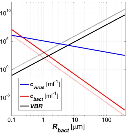
concentration of a phage-host pair in the environment is the radius of the bacterium (Fig. 1.1).
We found that the fixed point (i.e., steady state) concentration of bacteria scales as r-4 with r
being the radius of the bacterium. Since in nature, the radii of bacteria vary by over three orders
of magnitude, our model predicts that the concentration of bacteria can change by over 13 orders
of magnitude! Furthermore, our model predicts that large bacteria will be exceedingly rare, with
the largest known bacterium (Thiomargarita namibiensis having a diameter of 750 μm) predicted
to have one cell in ~103 liters of water. On the other hand, we predict that the concentration of
the viruses infecting large bacteria will be high enough so that, using molecular techniques, these
Figure 1.1. Scaling of the virus concentration, the bacterium concentration and the VBR with the radius of the bacterium for a single phage-host system. This figure shows that the radius of a bacterium is a critical parameter determining the fixed point concentration of the bacterium.
1.3.2 The biophysics of many phage-host systems
How many is many?
Thus far we have dealt with an artificial problem of a single phage-host system. In nature there
are many such systems and in Section 4.4 we deal with the question of how to make the
transition from a single phage-host system, to many such systems in the environment. How many
is many? In the Venter expedition to the Sargasso Sea, every sample containing several hundreds
of liters of ocean water was found to have at least 300 bacterial species (using a cutoff equivalent
to a small subunit rRNA cutoff of 3%) [26]. Therefore, we expect that a natural environment will
contain at least hundreds (probably thousands) of phage-host systems. Since the host range of
phages is narrow, these phage-host systems can be treated, to a first-order approximation, as
values, and that the fixed point concentration of bacteria is extremely sensitive to this parameter,
suggested to us that one cannot simply replace this parameter with an average value. One
actually needs to calculate this average using the probability density function of bacterial radii
for the given environment.
A simple evolutionary scenario
The difficulty in making the transition between a single phage-host system and many phage-host
systems in the environment, is figuring out what is the a priori probability density of radii in a
given environment, i.e., the probability per radius that a given environment a priori would
contain a bacterial species with this radius. This function (which we denoted by f rR ( )) has
evolutionary significance and can be interpreted as the density of bacterial species, perhaps
analogous to the density of states in statistical mechanics, and reflects the evolutionary history of
bacteria in the given environment. If the radii of all bacterial species that have adapted to survive
in the given environment were known, one could calculate this function. Since we cannot
calculate this function from first principles, we considered the simplest evolutionary scenario
where this function is a constant, which means there is no selection pressure on bacterial radii,
i.e., all radii are a priori equally probable. Given this assumption we were able to obtain
expressions for basic quantities, such as, the total concentration of bacteria in a given
environment, the total concentration of viruses in a given environment, the VBR, and the total
bacterial biomass in a given environment. These results are especially interesting given that they
The size spectra of bacteria in the ocean
One additional quantity that we can calculate given f rR ( ) is the distribution of radii in a given
environment, and from this function we can easily calculate the probability that a bacterium of
random volume V, is greater than or equal to a given volume, v, or Prob(V v≥ ). This function is
called the size spectra of radii and has been of interest to marine biologists for decades, with
measurements dating back to the work of Sheldon in 1972 [27]. In 2001 the Chisholm lab from
MIT measured the size spectra of microbes in the western north Atlantic Ocean. They found that
the size spectra obeyed a power law with a slope between -1 and -1.4. The ensemble average of
all environments was well described by a power law of slope -1.2. When expanding their dataset
to include microzooplankton the slope was corrected to a value close to -1. Our calculation,
given our simple evolutionary scenario, predicted a power law with a slope of -1, hopefully
indicating that we are on the right track.
Species richness
In section 1.2.2 we mentioned that the total concentration of bacteria is determined either by the
protists or by the availability of nutrients [15]. Thus, given the total concentration of bacteria in
an environment, one can in fact calculate the number of predicted species. By considering two
extreme models of spatial distribution of diversity — complete homogeneity and maximal
heterogeneity — we were able to calculate bounds on the total diversity in the ocean water
column. In Section 4.4 we also explore how the number of species scales with basic parameters
and found that, quite intuitively, warm, nutrient-rich environments where viruses have a long
lifetime will sustain the greatest diversity of species. Finally we compared estimates of diversity
What is a species?
When applying our model to data we realized that there is something strange about our
biophysical model. No where did we define what a “species” is! How different do two genomes
(bacterial or viral) need to be in order to be considered different “species”? It is this question that
we tried to address in Chapter 5.
1.4 The evolutionary perspective
1.4.1 A model for co-speciation of viruses and bacteria
In order to answer what a bacterial or viral species are, one needs to go to a higher theory that
takes into account the genetic aspect of these entities, and not just parameterize them with a
radius, decay rate, and so on. We therefore sought to formulate an evolutionary model that could
hopefully supply us with a definition of what is a species. This model needed to respect a few
basic rules so that it would be equivalent to our biophysical model. These rules were basically
that: (1) each bacterial species was associated with a single viral species and vice versa (i.e.,
there is no cross interaction between phage-host systems) and (2) each species (bacterial or viral)
was unique and distinguishable from all other species. We then asked ourselves the following
question: if we start from a state of a single bacterial species interacting with a single viral
species, how would this state evolve so that after some time we obtained a state comprised of
two bacterial species and two viral species, where the new species were independent of the old
species. Such an evolutionary model would create a “world” with single viral species paired
with single bacterial species, and vice versa, and where each bacteria-viral species pair was
independent of all other pairs. We found that in order for these strains to evolve we needed to (1)
define the concept of a “strain”, which is like a species, only there is no restriction on whom this
corresponding viral strain co-emerges so that the symmetry between bacteria and viruses is
conserved. By considering how a species evolved through generation of strains, into a new
species, a qualitative picture of what a species is, within the context of this model, emerged (Fig.
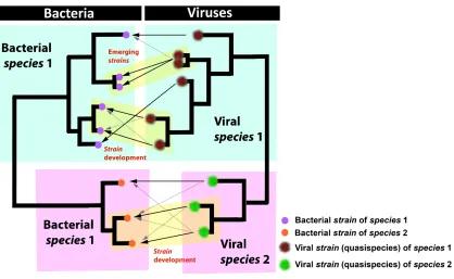
1.2; see also Fig. 5.1 that illustrates the process of co-speciation). How this complex structure
was obtained is discussed in detail in Chapter 5. When this structure is viewed in a genetic
coarse-grained way we recover the simple picture of our biophysical model: species interacting
uniquely with species. Therefore we argue that this model can be used to interpret the results of
the biophysical model. Such a situation is often encountered in physics, where one theory is the
limiting case of another (such as nuclear physics’ versus particle physics’ description of a
proton). Such limits are related to scale transformations in renormalization group theory,
Figure 1.2 Schematic depiction of bacterial and viral species and strains. The relation between bacterial and viral species and strains according to a postulated evolutionary model considered in Chapter 5. Each bacterial species interacts with a single viral species. Bacterial strains on the other hand (that are simply emerging bacterial species) are initially part of a mesh of interactions with other strains. The interaction of the bacterial strain with the co-evolving viral strain is critical in order for both strains to evolve away from this state into a state of mutual independence (emerging as new species).
1.4.2 Is positive feedback driving co-speciation?
Perhaps the most interesting finding of this model was that in order for a new bacterial species
and new viral species to co-emerge, the emerging bacterial and viral strains may be driving each
other’s evolution, through a positive feedback evolution mechanism. This positive feedback
causes the strains to evolve as fast as possible from their initial state in order to sever the bonds
with their parental strains and become independent (Fig. 1.3). This positive feedback evolution
mechanism is the arms race between bacteria and viruses. The logic behind our suggestion is the
1. Phages for some reason have converged to an evolutionary solution where they have a narrow
host range. This is not the most beneficial solution for a parasitic element, as a wide host
range, such as that of a grazer, would be much more effective. Therefore, there appears to be
some evolutionary advantage to this solution.
2. In the process of the arms race, viruses cause selective sweeps in the bacterial population.
Such bottlenecks are known to accelerate evolution as traits in small populations can be fixed
quickly. Thus, the phage is driving bacterial evolution, distancing the new bacterial strain as
fast as possible from the bacterial strain from which is was born (Fig. 5.1). This evolution is
necessary for the emerging bacterial species since this will lead the emerging viral species to
lose its affinity to the parental bacterial strain and gain control over it. As it gains control, the
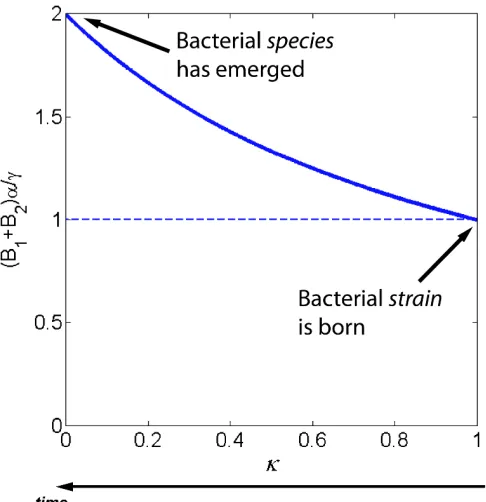
concentration of the emerging bacterial species increases (Fig. 1.4). The concentration of the
emerging bacterial species is maximal when the new viral species has total control over it.
Thus, this process allows the emerging bacterial species in the end to “take up” its own
concentration.
3. As the new viral species is emerging, it is controlling two populations, the parental bacterial
species and the new bacterial strain (Fig. 5.1). In order for this phage to form a unique
association with the new bacterial species (i.e., control only it) it must evolve away from its
current state as far as possible until it can no longer infect the parental bacterial strain. This
process appears to be achieved through the bacterial-viral arms race, since the new bacterial
strain is forcing the virus to keep muting in order to track the new bacterial strain and the
virus is causing the new bacterial strain to evolve.
4. Combining 2+3 we conclude that perhaps through positive feedback the bacterial and viral
state of two species (Fig. 5.1). Thus, viruses are the tool of evolution to generate species, and
the narrow host range of phages is necessary to achieve this goal.
Chaotic evolution?
Since a positive feedback mechanism amplifies noise exponentially (like the shrill of a
microphone in front of a speaker), the process of bacterial speciation may be simply a process of
“amplifying noise”. This may open the door to quantitative analysis via chaos theory. For
example, it would be interesting to see if phylogenic trees of bacteria spanning many orders
(strain, species, genus, family, order, etc.) display any features of self similarity, the hallmark of
fractals generated by chaos theory. Further quantities that may be tractable are the rate speciation
and the number of strains per species.
An experimental system to test the predictions of this theory would be Lenski-type evolution
experiments with E. coli + a lytic phage. Specific experiments are suggested in section 5.4. In
Figure 1.3 Positive feedback evolution model for emerging bacterial and viral “species”.
Figure 1.4. Total concentration “taken up” by the evolving bacterial strain and its parental strain.
Initially, the total concentration of the parental bacterial species (B1) and the just-emerging bacterial species (B2), in normalized units, is 1 and is determined by the controlling viral species. As the new bacterial strain is emerging, it is driving the evolution of the emerging viral strain,
causing its affinity to the parental bacterial strain to drop (i.e., κ, which is a measure of the
1.5 The experimental frontier
1.5.1 Phage-host co-localization methodology
Thus far, phage-host interaction in the wild could only be investigated for certain systems such
as cyanophages [28,29,30,31]. The challenge lays in the fact that traditional techniques in
microbiology necessitate that hosts be culturable in order to isolate their phage. Yet when >99%
of bacteria cannot be cultured [32] other methods need to be sought. In Chapter 2 we describe a
method using digital microfluidic PCR array to pair phages with their bacterial host without
having any prior assumptions regarding the host. The experimental scheme for a new
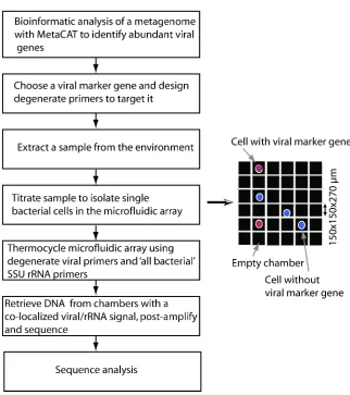
environment is shown in Fig. 1.5.
The first stage involves obtaining a metagenome for the environment of interest. Once gene
objects have been assembled and translated, one can run a bioinformatic tool called MetaCAT
(Chapter 3) that was written for this purpose. MetaCAT (metagenome cluster analysis tool) is
used to find the most abundant viral genes in a given metagenome by clustering together similar
genes in the metagenome that are expected to be related (Fig. 1.6). This tool is used to find
candidate viral marker genes. The idea behind using this tool for viral genes is that viral genes
tend to have many mutations, and therefore are not collapsed by the assembler. Therefore we
expect that the abundance of the genes in the metagenome reflects their abundance in the sample.
Thus abundant viral genes found by MetaCAT would correspond to abundant and thus dominant
genes in the sample. Furthermore, the more alleles one has for primer design, the more general
Figure 1.5 Workflow using the microfluidic digital PCR array for host-virus co-localization in a novel environmental sample
After degenerate primers have been designed, one can load an environmental sample onto a
digital PCR microfluidic array panel, which distributes the sample evenly among 765 6 nl
chambers. Samples are titered such that a small fraction of chambers contain a single cell that is
probed for a universal small subunit rRNA gene and a viral marker gene. In Fig. 1.7 we show a
typical digital PCR panel after PCR cycling. Each chamber that contains both colours (red for a
viral marker gene and green for the small subunit rRNA gene) is a potential co-localization
phylogenetic analysis. The great challenge with this experiment was that the phage gene
displayed many mutations from cell to cell of the same host species. Therefore we needed to
devise a statistical criterion and sampling strategy to separate repeated co-localizations due to
chance from genuine co-localization.
Figure 1.6 Ideal clustering of gene objects in a metagenome. Each dot represents a gene object in a metagenome, with the entire metagenome depicted by the blue oval. Similar genes are grouped into clusters (circles of different colors) and each cluster is represented by a single gene from a known reference database. In this schematic description, the distance between dots is interpreted in an abstract manner and does not correspond to a rigorous metric.
1.5.2 The case of the termite hindgut
The co-localization experiment described in Chapter 2 was performed for samples from the gut
of a termite. Our analysis of the termite hindgut began by analyzing the metagenome of a higher
termite collected from Costa Rica. This analysis detected several highly abundant unique viral
genes. We then BLASTed these genes against the genomes of two spirochetes that were isolated
homologs: a portal protein and a terminase protein. These two genes were part of larger
[image:33.612.129.500.143.420.2]prophage-like elements (two elements in each genome). We then proceeded to uncover the entire
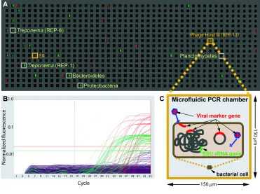
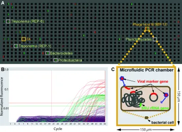
Figure 1.7. End-point fluorescence measured in a panel of a microfluidic digital PCR array. A. The measured end-point fluorescence from the rRNA channel (right half of each chamber) and the terminase channel (left half of each chamber) in a microfluidic array panel. B.
Normalized amplification curves of all chambers (red/viral, green/rRNA). C. Specific physical associations between a bacterial cell and the viral marker gene resulting in co-localization include for example: an attached or assembling virion, injected DNA, an integrated prophage or a plasmid containing the viral marker gene.
prophage-like element in each genome (Fig. 1.8). To show that these prophage-like elements
were also abundant in the metagenome we BLASTed each gene from in the prophage-like
element against the metagenome. The result, shown in Fig. 1.8, indicated that these
prophage-like elements were indeed abundant in both termites. We chose the terminase gene to be our viral
marker gene and designed degenerate primers to amplify a large portion of this gene (~820 bp).
tested these primers against nine termite species belonging to seven families collected from five
different geographical locations. Fig. 1.9 shows that indeed we obtained positive hits for all these
termites confirming that this prophage-like element is ubiquitous to termites (at least of north and
central America). We also obtained a positive hit for a wood feeding roach, raising the
possibility that this prophage-like element has infected a common ancestor of termites and wood
feeding roaches and has been transformed since. In Chapter 2 we describe the results of our
co-localization experiment gut samples extracted from Reticulitermeshesperus using the same viral
[image:34.612.64.532.309.546.2]primers.
Figure 1.9.Agarose gel electrophoresis analysis of terminase PCR product amplified from termite and related insect species. PCR product using degenerate primers ter.7F and ter.5eR targeting the large terminase subunit gene. Specimens included were: Nasutitermes sp.
(cost003), Rhynchotermes sp. (cost004), Microcerotermes sp. (cost008), Amitermes sp. (cost010), Periplanetaamericana (croach), Cryptocercuspunctulatus (wfroach), Reticulitermes hesperus (retic), Incisitermes minor (incis), Gnathiamitermes sp. JT5 (JT). ZAS9 was used as a positive control. Also shown are two negative PCR controls.
1.6 Stress fibers in single fibroblast cells
Dr. Blake W. Axelrod, a research engineer in the Roukes lab, built a microfluidic NEMS device
allowing him to measure the force as a function of time of a stress fiber in a single fibroblast cell,
performing the highest resolution measurement to date. In this experiment, a single fibroblast
cell (Fig. 1.10A insert) contacts a NEMS force sensor. When the cell is placed in a recovery
medium it exerts a force on the force sensor (Fig. 1.10A, blue region) corresponding to the force
generated by an assembled stress fiber (about 20nN). Once a substance called cytochalasin D is
flowed in, the stress fiber undergoes disassembly and consequently the force declines (Fig.
1.10A, red region). The process of disassembly is a reversible one, since when flowing the
examined more closely, each assembly/disassembly profile appears to be comprised of steps that
appear to, on average, increase in duration (Fig. 1.10B). These steps were remarkably uniform in
the force amplitude and it was postulated that they are the result of individual sarcomeres failing
or contracting.
At the time the data was presented it was not clear what the origin of the temporal dynamics is,
what the mechanism leading to exponential-like “charging” and “discharging” curves is, and
why the steps are increasing with time. In Chapter 6 we present our analysis of Blake’s dataset.
We proposed a simple stochastic model for stress fiber assembly and disassembly, whereby
individual sarcomeres assemble or dissemble (a) abruptly, (b) irreversibly, (c) independently, (d)
with the time to the event of assembly or disassembly exponentially distributed with a fixed time
constant (Fig. 1.11). With this model it is simple to explain why, for example, steps increase in
time. According to this model, in the case of stress fiber disassembly for example, the time from
the perturbation (t=0) until a sarcomere fails is exponentially distributed. If there are N
sarcomeres, then at t=0 there are N independent sarcomeres that can fail. Thus one needs to wait
a short period of time to observe a step. As more steps fail, one needs to wait longer until one
sees a step because there are less remaining sarcomeres. In Chapter 6 we show that the inverse
duration times of each step increase linearly with time. In Fig. 1.12 we show the inverse duration
times versus the linear prediction of the model (where parameters were estimated from the data
based on the model). The data appears to be behaving qualitatively as predicted. In Chapter 6 we
present more rigorous tests to check our model. We show the (a) sarcomeres appear to be failing
or assembling statistically as exponential variables. (b) When data was rescaled using model
Figure 1.10 Typical force-time response to Cytochalasin D perturbation. A. Typical measured force response to the force disruptor Cytochalasin D (red region) and recovery medium (blue region). Cytochalasin D belongs to a class of substances called Cytochalasins that are fast acting and reversible disruptors of contractile force. When Cytochalasin D is flowed in, the force decays due to stress fiber disassembly. When recovery medium is flowed in, the stress fiber reassembles and the force increases with time. Inset shows fluorescent image of the cell attached to the beam taken immediately before data acquisition, scale bar is 10 μm. B. Steps during CD-induced force collapse (upper) or force recovery (lower). The average step size is 1.08 nN ± 0.18 nN (n=96). Figure and caption courtesy of Blake Axelrod (Roukes lab, Caltech).
Figure 1.11. Schematic model for stress fiber relaxation. (1) Each sarcomere assembles or disassembles abruptly and irreversibly. (2) Sarcomeres assemble or disassemble independently of each other. (3) The time until a sarcomere assembles or disassembles is exponentially distributed (reflecting a certain constant probability rate for this event to occur). (4) The time constant for assembly is the same for all sarcomeres. Similarly, the time constant for disassembly is the same for all sarcomeres.
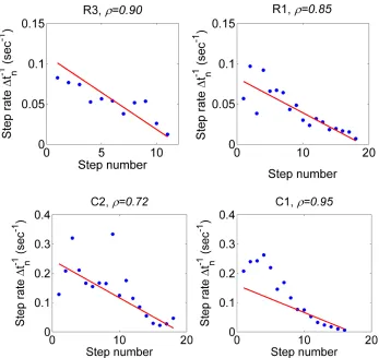
Figure 1.12. Stochastic model prediction of force step durations versus experimental data.
The stochastic model prediction for the inverse of the force step durations (red curve) versus experimental data points (blue dots). ρ is the Pearson correlation coefficient measuring the strength of the correlation. The red line is not a fit, as these lines were predicted based on parameters that were estimated from the data according to our stochastic model. Note that we anticipate a high level of noise since the standard deviation equals the predicted rates.
1.7 References
1. Weinbauer M (2004) Ecology of prokaryotic viruses. FEMS Microbiology Reviews 28: 127-181.
2. Danovaro R, Corinaldesi C, Luna GM, Magagnini M, Manini E, et al. (2009) Prokaryote diversity and viral production in deep-sea sediments and seamounts. Deep Sea Research Part II: Topical Studies in Oceanography 56: 738-747.
3. Klieve AV, Swain RA (1993) Estimation of ruminal bacteriophage numbers by pulsed-field gel electrophoresis and laser densitometry. Applied and Environmental Microbiology 59: 2299.
5. Fuhrman J (1999) Marine viruses and their biogeochemical and ecological effects. Nature 399: 541-548.
6. Suttle C (2007) Marine viruses—major players in the global ecosystem. Nat Rev Microbiol 5: 801-812.
7. Wommack K, Colwell R (2000) Virioplankton: viruses in aquatic ecosystems. Microbiology and Molecular Biology Reviews 64: 69.
8. Suttle CA, Chan AM (1994) Dynamics and distribution of cyanophages and their effect on marine Synechococcus spp. Applied and Environmental Microbiology 60: 3167.
9. Danovaro R, Dell'Anno A, Corinaldesi C, Magagnini M, Noble R, et al. (2008) Major viral impact on the functioning of benthic deep-sea ecosystems. Nature 454: 1084-1087.
10. Edwards R, Rohwer F (2005) Viral metagenomics. Nat Rev Microbiol 3: 504-510.
11. Casjens S (2003) Prophages and bacterial genomics: what have we learned so far? Molecular Microbiology 49: 277-300.
12. Wilcox R, Fuhrman J (1994) Bacterial viruses in coastal seawater: lytic rather than lysogenic production. Marine Ecology-Progress Series 114: 35-35.
13. Suttle C (2005) Viruses in the sea. Nature 437: 356-361.
14. Paul J, Kellogg C (2000) Ecology of bacteriophages in nature. Viral Ecology: 211–246. 15. Pernthaler J (2005) Predation on prokaryotes in the water column and its ecological
implications. Nature Reviews Microbiology 3: 537-546.
16. Thingstad T, Lignell R (1997) Theoretical models for the control of bacterial growth rate, abundance, diversity and carbon demand. Aquatic Microbial Ecology 13: 19-27.
17. Suttle C (2000) Ecological, evolutionary, and geochemical consequences of viral infection of cyanobacteria and eukaryotic algae. Viral Ecology: Academic Press. pp. 247–296.
18. Kutter E, Sulakvelidze A (2005) Bacteriophages: biology and applications: CRC Press.
19. Thingstad T (2000) Elements of a theory for the mechanisms controlling abundance, diversity, and biogeochemical role of lytic bacterial viruses in aquatic systems. Limnology and Oceanography: 1320-1328.
20. Weinbauer MG, Rassoulzadegan F (2004) Are viruses driving microbial diversification and diversity? Environmental Microbiology 6: 1-11.
21. Sorek R, Kunin V, Hugenholtz P (2008) CRISPR—a widespread system that provides acquired resistance against phages in bacteria and archaea. Nature Reviews Microbiology 6: 181-186.
22. Heidelberg JF, Nelson WC, Schoenfeld T, Bhaya D (2009) Germ warfare in a microbial mat community: CRISPRs provide insights into the co-evolution of host and viral genomes. PLoS One 4: e4169.
23. Banfield J, Young M (2009) Variety--the Splice of Life--in Microbial Communities. Science 326: 1198.
24. Weinbauer M, Peduzzi P (1994) Frequency, size and distribution of bacteriophages in different marine bacterial morphotypes. Marine Ecology Progress Series 108: 11-20.
25. Weinbauer M, Hoefle M (1998) Size-specific mortality of lake bacterioplankton by natural virus communities. Aquatic Microbial Ecology 15: 103-113.
26. Venter JC, Remington K, Heidelberg JF, Halpern AL, Rusch D, et al. (2004) Environmental genome shotgun sequencing of the Sargasso Sea. Science 304: 66.
28. Sullivan M, Huang K, Ignacio-Espinoza J, Berlin A, Kelly L, et al. (2010) Genomic analysis of oceanic cyanobacterial myoviruses compared with T4-like myoviruses from diverse hosts and environments. Environ Microbiol 12: 3035-3056.
29. Lindell D, Jaffe J, Coleman M, Futschik M, Axmann I, et al. (2007) Genome-wide expression dynamics of a marine virus and host reveal features of co-evolution. Nature 449: 83-86.
30. Angly F, Felts B, Breitbart M, Salamon P, Edwards R, et al. (2006) The marine viromes of four oceanic regions. PLoS Biol 4: e368.
31. Williamson S, Rusch D, Yooseph S, Halpern A, Heidelberg K, et al. (2008) The Sorcerer II Global Ocean Sampling Expedition: metagenomic characterization of viruses within aquatic microbial samples. PLoS ONE 3: 1456.
Chapter 2
Probing Individual Environmental Bacteria for
Viruses Using Microfluidic Digital PCR
2.1 Abstract
Viruses may very well be the most abundant biological entities on the
planet. Yet neither metagenomic studies nor classical phage isolation techniques have
shed much light on the identity of the hosts of most viruses. We used a microfluidic digital
PCR approach to physically link single bacterial cells harvested from a natural
environment with a viral marker gene. When we implemented this technique on the
microbial community residing in the termite hindgut, we found genus-wide infection
patterns displaying remarkable intra-genus selectivity. Viral marker allelic diversity
revealed restricted mixing of alleles between hosts indicating limited lateral gene transfer
of these alleles despite host proximity. Our approach does not require culturing hosts or
viruses and provides a method for examining virus-bacterium interactions in many
2.2 Introduction
Despite the pervasiveness of bacteriophages in nature and their postulated impact on
diverse ecosystems (1), we have a poor grasp of the biology of these viruses and their host
specificity in the wild. Though significant progress has been made with certain host-virus
systems such as cyanophages (2-5), this is the exception rather than the rule. Conventional
plaque assays used to isolate environmental viruses are not applicable to >99% of
microbes in nature since the vast preponderance of the microbial diversity on Earth has yet
to be cultured in vitro (6). Given the magnitude of the problem, the development of
high-throughput, massively-parallel sequencing approaches that do not rely on cultivation to
identify specific virus-host relationships are required. While m
2.3 Proposed method for phage-host co-localization
etagenomics has
revolutionized our understanding of viral diversity on Earth (7-9), that approach has as yet
done little to shed light on the nature of specific viral-host interactions, except in restricted
cases (10).
Recent advances in microfluidic technology have enabled the isolation and analysis of
single cells from nature (11-13). Here we present an alternative to the classical phage
enrichment technique where we propose to use an uncultured virus to capture its hosts
from the environment using a microfluidic PCR approach called digital multiplexPCR
(12, 14). To this end, microbial cells were harvested directly from the environment,
diluted and loaded onto a digital PCR array panel containing 765 PCR chambers operating
at single-molecule sensitivity. Samples were diluted such that the majority of chambers
were ideally either empty or contained a single bacterium (Fig. 2.1), achieving a Poisson
degenerate primers (17) were designed to target a subgroup of diverse phage-like elements
(18).
2.4 Hunting for phages in the termite hindgut
Concurrently, the small subunit ribosomal RNA (SSU rRNA) gene encoded by each
bacterial cell was amplified using universal “all bacterial” primers (see Fig. 2.4 for
experimental design). Possible genuine host-virus associations detectable by this assay are
depicted in Fig. 2.1C. Free phages may also co-localize with hosts, however these events
are not expected to lead to statistically significant co-localizations due to the random
nature of these associations (19).
The system we chose to investigate was the termite hindgut. This microliter-in-scale
environment contains ~107 prokaryotic cells per μl (20) with over 250 different species of
bacteria (21), making it ideally suited to explore many potential, diverse phage-host
interactions. To find a viral marker gene relevant to such an environment, the more
abundant candidate viral marker genes present in the sequenced metagenome from a
hindgut of a highertermite from Costa Rica collected in 2005 (22) were examined (Table
2.2; search algorithm described in the Materials and methods section). We then checked if
any of these viral genes had homologous counterparts in the sequenced genomes of two
spirochetes isolated in 1997 from a laboratory colony of a genetically and geographically
distant termite originally collected in 1986 from Northern California (23-24). We
identified two such genes encoding a large terminase subunit protein (homologous to the
T4 associated pfam03237 Terminase_6) and a portal protein (homologous to pfam04860
Phage_portal) exhibiting about 70–78% amino acid identity to their closest homologs in
the higher termite gut metagenome (Table 2.3). This finding is surprising given that
exhibit little overall sequence similarity (25-28). Further analysis revealed that the
spirochete viral genes were part of a larger prophage-like element, with the majority of
recognizable genes most closely related to Siphoviridae phage genes (19). The association
of these genes with prophage-like elements is consistent with the fact that both the
Terminase_6 pfam and the Phage_portal pfam describe proteins in known lysogenic and
lytic phages.
As a viral marker gene for this prophage-like element we chose the large terminase
subunit gene. This gene is a component of the DNA packaging and cleaving mechanism
present in numerous double-stranded DNA phages (26) and is considered to be a signature
of phages (29). We consequently designed degenerate primers based on the collection of
fifty metagenome and treponeme-isolate alleles of this gene. The ~820bp amplicon
spanned by these primers covered about two thirds of this gene and approximately 77% of
the predicted N-terminal domain containing the conserved ATPase center (26, 30), the
“engine” of this DNA packaging motor (31) (see alignments in Figs. 2.5 and 2.6). Testing
these primers against the RefSeq viral database (32) did not yield any hits (Fig. 2.5).
Indeed, the closest homolog of this gene in the RefSeq viral database displayed only 25%
amino acid identity (Table 2.3). Thus, while this terminase gene was clearly associated
with the Terminase_6 pfam, the termite related alleles appear to be part of a novel
assemblage of terminase genes in this environment and not closely related to previously
Figure 2.1. End-point fluorescence measured in a panel of a microfluidic digital PCR array.A. The measured end-point fluorescence from the rRNA channel (right half of each chamber) and the terminase channel (left half of each chamber) in a microfluidic array panel. Each panel in the array (one of twelve) consists of 765 150 x 150 x 270μm3 (6 nL)
reaction chambers. Retrieved co-localizations are outlined in orange and positive rRNA chambers randomly selected for retrieval are outlined in gray. FA indicates false alarm (a probable terminase primer-dimer). B. Normalized amplification curves of all chambers in (A) after linear derivative baseline correction (red/viral, green/rRNA). C. Specific physical associations between a bacterial cell and the viral marker gene resulting in co-localization include for example: an attached or assembling virion, injected DNA, an integrated prophage or a plasmid containing the viral marker gene.
Given that terminase genes of different phages often exhibit less sequence similarity (see
above), the fact that we found such closely related terminase genes from such distantly
related termites collected from well separated geographical locations (California and Costa
Rica) and from specimens collected almost two decades apart led us to speculate that this
family of viral genes and prophage-like elements might be ubiquitous in termites. Indeed,
to date we have identified close homologs of the large terminase subunit gene in the gut
different geographical locations. We therefore wished to identify the bacterial hosts
associated with this viral marker gene. To this end, we made collections of representatives
of a third previously unexamined termite family (Rhinotermitidae; Reticulitermes
hesperus, from a third geographical location in Southern California) over a span of six
months (Table 2.4). We then performed seven independent experiments, where in each
case the hindgut contents of three worker termites were pooled, diluted, and loaded onto a
digital PCR array, screening in total ~3000 individual hindgut particles (i.e., individual
cells or possibly clumps of cells positive for the SSU rRNA gene).
2.5 Identification of novel uncultured bacterial hosts
Of the 41 retrieved co-localizations, 28 were associated with just four phylotypes
designated “Phage Hosts I, II, III and IV” (see Fig. 2.2, Table 2.1 and the phylogenetic
analysis in Fig. 2.7 and Tables 2.5 and 2.6). Statistically, the reproducible
co-amplifications were significant and cannot be explained by random co-localization of two
unassociated genes (Table 2.1). Furthermore, these associations were independently
reproduced in specimens from different colonies collected six months apart (Fig. 2.2),
indicative that relationships between specific host bacteria and viral markers were being
revealed.
All four of the phylotypes were members of the spirochetal genus Treponema and
exhibited significant diversity within this genus (Table 2.5). No reproducible or
statistically robust associations involving other bacteria were observed. The terminase
alleles that associated with these cells shared ≥69.8% identity (average 81.9 ± 8.3%
(Fig. 2.5), suggesting that the primer set amplifies elements exclusively found associated
with termite gut treponemes. Analysis of the retrieved terminase gene sequences reveal
that they are under substantial negative selection pressure with ω=β/α=0.079, where ω is
the relative rate of non-synonymous, β, and synonymous, α, substitutions (18)(see Table
2.7 for additional estimates for individual hosts). Furthermore, none of the terminase
sequences in Fig. 2.2 appeared to encode either errant stop codons or obvious frame shift
mutations, and functional motifs appeared to be conserved (Fig. 2.5). Together, the
sequence data suggest that these genes have been active in recent evolutionary history and
are not degenerating pseudogenes (19).
*Based on the DOTUR analysis described in Table 2.5
†Based on the DOTUR analysis described in Table 2.6. Reference library frequencies are roughly 1/3 of the co-localization frequencies indicating that sampling was unbiased.
‡The statistical test to determine the P value is explained in the supporting text.
Since the viral marker gene was present in hosts spanning a swath of species of termite gut
treponemes, we were interested to see if this viral marker exhibited any selectivity within
this genus. The relative frequency of free-living Treponema phylotypes was determined
by randomly sampling chambers positive for the rRNA gene (18) (Fig. 2.3, Fig. 2.7). We
found that Hosts I through IV were relatively infrequent, comprising 1.3% to 6.4% of the
sampled Treponema cells (Table 2.1) and collectively about 9.8% of the sampled bacterial
cells (correcting for reagent contaminants). Interestingly, the three most abundant
Table 2.1 | Statistics of repeatedly co-localized SSU rRNA genes
Host co-localizationsNo. of repeated *
(n=41)
Occurrence in reference library†
(n=118)
P value (one tailed, n=41)‡
Host I 13 5 5.4x10⁻¹⁸
Host II 8 2 7.6x10
Host III
-13
4 1 5.7x10
Host IV
-7
Treponema phylotypes in the survey constituting ~30, 10 and 9% of the free-swimming
spirochetal cells (REPs 1, 2 and 3 in Fig. 2.3; see also Fig. 2.7 and Table 2.6) were never
co-retrieved with the viral marker gene, to the extent that this target was spanned by our
degenerate primers. Given that the degenerate core region (17) of each primer targets
residues that were strictly conserved in gut microbes of highly divergent termite
specimens (Fig. 2.5), and that these primers successfully amplified this gene from the guts
of many different termite species (see above), it appears that these strains are most likely
either insensitive to this virus or that only a small percentage are infected (19). Therefore
we conclude that ~50% of the free-swimming spirochetal cells in the gut were likely not
infected with an element encoding the targeted viral marker gene, whereas ~12% were
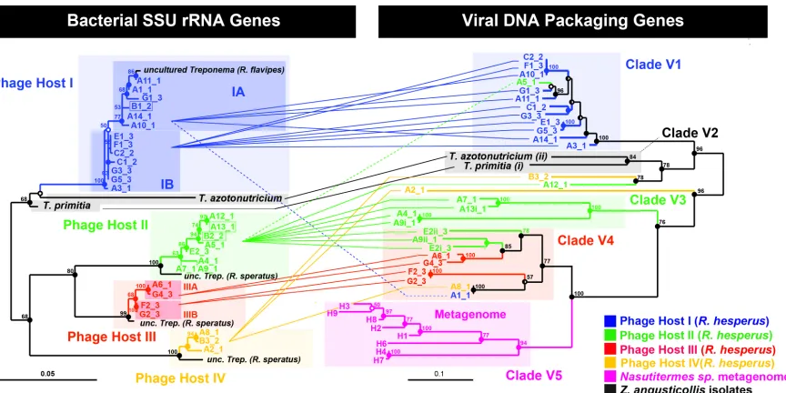
Figure 2.2. Phylogenetic relationship between cultured and uncultured bacterial host rRNA genes and their associated viral DNA packaging genes. Left: Maximum Likelihood (ML) tree of 898 unambiguous nucleotides of the SSU rRNA gene of ribotypes that repeatedly co-localized with the terminase gene, including the two isolated spirochetes Treponema primitia and Treponema azotonutricium. Shorter sequences (A7, 780bp and A9, 806bp) were added by parsimony (dashed branches). Right: ML tree of 705 unambiguous nucleotides of the large terminase subunit gene. Connecting lines represent co-localized pairs, revealing restricted mixing of terminase alleles between different bacterial hosts. For association of three additional recombinant sequences (boxed on the left) see Fig. 2.8. Statistically we estimate that an average of 0.6 co-localizations are false (~2% error (19)). The sequence error rate (40) for the rRNA and terminase genes was measured to be 0 (n=8) and <0.6±0.3% SD (n=9), respectively (18). Alleles are named by array (A–G) and retrieval index followed by an underscore and the colony number (colony 1 being sampled six months prior to colonies 2 and 3). Lower-case Roman numerals indicate multiple terminases per chromosome. Scale bars represent substitutions per alignment. For interpretation of node support refer to (18) and for accession numbers Table 2.11.
2.6 Phage-host cophylogeny
To elucidate the evolutionary relationship between the terminase alleles and their hosts we
examined the phylogeny of the terminase genes associated with each bacterial host.
Terminase alleles from R. hesperus formed separate clades from the clades of the two
hesperus, different bacterial hosts exhibited different patterns of viral allelic diversity.
Terminase sequences associated with Host I, for exam